Resolution-intensity optimisation on quasielastic neutron scattering spectrometers

1. Introduction

Quasielastic Neutron Scattering (QENS) spectroscopy [2,12] is an important tool for studying the microscopic dynamics of condensed matter. Because the measured quantity, the scattering function S ( Q , ω ) , depends on the scattering vector Q as well as on the frequency ω QENS provides a structural information for the studied process in addition to the dynamical.

On the other hand, QENS has a more restricted dynamical range than non-Q-dependent spectroscopic methods. QENS spectrometers usually cover 2…3 decades in frequency [14] while e.g. dielectric spectroscopy covers more than 12 [8]. Therefore, considerable effort has been taken to improve the energy resolution of such spectrometers which is directly related to the frequency resolution by Δ ω = Δ E / ℏ .

Nowadays, many QENS instruments offer the possibility to adapt the energy resolution to the specific dynamics to be studied. Especially, instruments where the incident energy is defined by neutron time-of-flight and the energy after scattering is measured by time-of-flight, ToF-ToF instruments, allow varying the resolution in a broad range [4,6,7,9]. In such instruments there is an inevitable trade-off between resolution and registered intensity, i.e. counting statistics. When the resolution is improved the counting statistics is worsened and vice versa.

Until now, there is no rational criterion established how to handle this balance between resolution and statistics. In this paper a simple guide line is developed for the choice of the resolution on such instruments.

Of course, there are QENS instruments (e.g. backscattering) which do not allow a change of the resolution or at least not in an easily practicable way. For such instruments the calculations presented here will still give some helpful information, e.g. on the registration time necessary for achieving a certain accuracy. Also, they may be valuable for the construction of new instruments to determine beforehand whether an optimisation of resolution or intensity is more desirable.

2. Quality of QENS spectra

Arguably, there is no general definition of the quality of a QENS spectrum. But it is clear that two factors come into play: the energy resolution and the overall statistical errors. Usually an improvement of the resolution, e.g. by narrowing an energy filter, leads to a decrease in statistical quality. The crucial question is how to weigh one against the other, e.g. a better resolution against worse counting statistics. Here, it is proposed to do this based on a quality measure defined via the (inverse) Fourier transform of the spectrum as the maximal time at which the errors in the intermediate scattering function calculated from the experimental data are still tolerable. It is clear that this time is reduced by a worse resolution directly and indirectly by increasing error bars at large times.

It is understood that this measure is not perfectly fitting every application of QENS. In the particular case also more subtle features as the unavoidable correlation of errors introduced by the Fourier transform in S ( Q , t ) may play an important rôle. Also what finally matters is the quality of model parameters determined by a fit of the data. This may depend on more characteristics of the error distribution which are not considered here. Nevertheless, this paper aims at a general expression without regard to the specific physical background of the measurement in the hope that a simple criterion for the estimation of the optimal resolution has a better chance to be employed than a complex calculation which is probably too cumbersome to be carried out.

Consider a neutron scattering spectrometer with a resolution function R ( ω ) and a scattering function S ( ω ) to be measured. (Throughout this paper, the scattering vector (Q) dependence will be omitted. So, S ( ω ) represents S ( Q , ω ) for a certain detector. Similarly, S ( t ) should be read as S ( Q , t ) . Of course, there may be situations where the Q range provides an argument which overrides the considerations presented here. E.g. improvement of the resolution may require a larger incident wavelength which impedes access to the Q necessary to study the system. Such arguments are impossible to quantify in a general way and will not be considered.) Assuming an energy independent resolution, the observed spectrum is the convolution of the scattering function and the resolution function [12], (1) S ˜ ( ω ) = ∫ − ∞ ∞ S ( ω − ω ′ ) R ( ω ′ ) d ω ′ . From the convolution theorem [3] follows that the intermediate scattering function can be obtained by inverse Fourier transform from the inverse Fourier transforms of the experimental data (2) S ( t ) = S ˜ ( t ) / R ( t ) where S ˜ ( t ) and R ( t ) are the inverse Fourier transforms of the experiment on the sample to be studied and a resolution experiment. The latter may be done with the sample itself at low temperature (where S ( ω ) = const . × δ ( ω ) in classical approximation) or with a sample which scatters predominantly elastically (e.g. vanadium).

The experimental raw data are the numbers of neutrons counted in the energy channels. (For simplicity, in the following this number will be called ‘counts’.) Considering an energy channel b k < ω < b k + 1 nominally centred at ω = c k the counts will be (3) I k = I · ∫ b k b k + 1 R ( ω ) d ω for the resolution experiment and (4) J k = I · ∫ b k b k + 1 S ˜ ( ω ) d ω for the sample. Here, I is the overall ‘intensity’ of the instrument. Among various factors, it contains the measuring time, the primary flux and the resolution-dependent energy selection of neutrons.

The inverse Fourier transforms in (2) will be calculated numerically as (5) R ( t ) = 1 I ∑ k I k exp ( i c k t ) and (6) S ˜ ( t ) = 1 I ∑ k J k exp ( i c k t ) , respectively. The exact formula used may differ (e.g. the trapezoid rule may be used for the integral) but the basic procedure is reflected in formulae (5) and (6).

For a normalised resolution function which does not extend beyond the energy range of the spectrometer the total intensity is (7) ∑ k I k = I . It is more difficult to state the same total (8) J = ∑ k J k for the sample. If the resolution is measured with the sample itself at low temperature and otherwise same instrumental conditions, one expects J ≲ I . If the coherent structure factor does not change with temperature and all inelastically scattered intensity still falls into the range of the instrument, J = I . But because the last condition is usually not fulfilled, there is a decrease with temperature. Because of thermal expansion, S ( Q ) will also not be constant resulting in a small increase or decrease. If the resolution is measured on a different material (e.g. a vanadium standard) any value is possible. But since one does not want to spoil the experiment with a bad resolution, conditions are normally chosen such that J and I still have the same magnitude.

With the definitions above, it is possible to calculate the error of S ( t ) by error propagation through (5), (6), and (2): (9) Δ S ( t ) = ∑ k J k exp ( i c k t ) ∑ k I k exp ( i c k t ) ∑ k ( Δ J k ) 2 | exp ( i c k t ) | 2 | ∑ k J k exp ( i c k t ) | 2 + ∑ k ( Δ I k ) 2 | exp ( i c k t ) | 2 | ∑ k I k exp ( i c k t ) | 2 . At this point it has to be considered that R ( t ) may be complex if R ( ω ) is not symmetric. Also S ( t ) is complex because the detailed balance relation S ( Q , − ω ) = exp ( ℏ ω / k B T ) S ( Q , ω ) makes the scattering function asymmetric. (The latter fact is often neglected because in typical QENS experiments ℏ ω ≪ k B T .) To take this into account the error of S ( t ) has to be understood as the square root of the sum of the squared errors in the real and imaginary part. The errors of the counts can be expressed as usual, e.g. Δ I k = I k , | exp ( i c k t ) | = 1 , and some of the sums can be replaced by the total values J and I. Finally, all numerical expressions can be approximated by the expected exact values: (10) Δ S ( t ) = | S ( t ) | J I 2 | R ( t ) | 2 | S ( t ) | 2 + 1 I | R ( t ) | 2 = | S ( t ) | 2 + J / I I | R ( t ) | . At that point it would be nice to have an expression which only includes I and R ( t ) because this would directly reflect the interplay of resolution and intensity, independently of the specific experiment. But the numerator still contains S ( t ) , reflecting the actual dynamical properties of the sample, and J / I , depending on the way the resolution function is determined. But as explained above for a typical experiment J / I ∼ 1 . For incoherent scattering | S ( t ) | = 0 … 1 , for coherent scattering | S ( Q , t ) | = 0 … S ( Q ) with maximal values not exceeding one too strongly (unless Bragg peaks are present). So the numerator may be replaced by 2 to reflect a typical experiment: (11) Δ S ( t ) = 2 I | R ( t ) | . (This can also be justified from the fact that the experimenter will adjust measuring times in a way that the errors contributed by the actual sample run are equal to those from the resolution run.) Note that, since | R ( t ) | decreases monotonically, the error increases with t.

In order to simplify the notation | R ( t ) | will be written as R ( t ) in the following. The examples in Sections 3 and 4 will deal with symmetric R ( ω ) anyway so that this does not make a difference. For asymmetric resolution functions (e.g. for instruments on pulsed sources) one has to keep in mind that for the purpose here, R ( t ) is the absolute value of (5) and not its real part.

Finally, it is proposed to define the quality of a neutron scattering spectrum as the time where the error in the intermediate scattering function exceeds a threshold ϵ: (12) t max = R − 1 ( 2 ϵ I ) . (Here, R − 1 ( z ) is the inverse of R ( t ) , not the reciprocal.) At that point, the choice of ϵ is somewhat arbitrary and will depend on the objective of the experiment. Together with the arbitrariness of the numerator 2 , this leaves t max not well defined. Nevertheless, one may expect that for a comparison where ϵ is not varied, t max allows to rate the trade-off between intensity and resolution width in an objective way.

In practice, the relation between the resolution function R ( ω ) and the intensity factor I may be complicated. For simplification it is assumed that R ( ω ) only depends on a single parameter σ, the resolution width, and does so fulfilling an affine scaling: (13) R ( ω ) = 1 σ R ˆ ( ω σ ) which means after inverse Fourier transform: (14) R ( t ) = R ˆ ( σ t ) . With this simplification, the resolution width simply enters as a reciprocal factor into the maximally accessible time: (15) t max = 1 σ R ˆ − 1 ( 2 ϵ I ( σ ) ) where R ˆ − 1 ( x ) is the inverse master function of the resolution of the instrument.

3. An example: Lorentzian resolution

A simple example for the resolution function of a neutron scattering spectrometer would be the Lorentzian function (a.k.a. Cauchy distribution): (16) R ( ω ) = 1 π σ 1 1 + ( ω / σ ) 2 . Here, σ has the concrete meaning of the half width at half maximum (HWHM). Its inverse Fourier transform is (17) R ( t ) = exp ( − σ t ) and the master function is R ˆ ( x ) = exp ( − x ) .

For this example it is assumed that one can continuously vary the resolution and that the total intensity is proportional to the square of the width (18) I ( σ ) = I 1 σ 2 . This assumption is founded in the concept of a monochromator and an analyser both reducing the number of selected neutrons proportionally to σ.

OPEN IN VIEWER

Fig. 1.

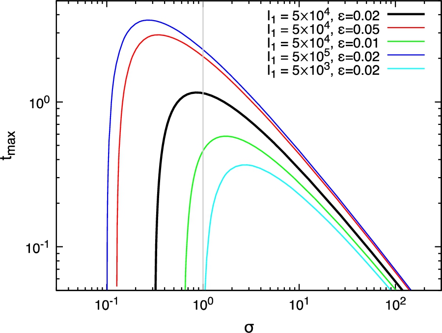
Maximal inverse Fourier time for different combinations of intensity factor and required accuracy of S ( t ) . Black, bold curve: I 1 = 5 × 10 4 , ϵ = 0.02 , red: I 1 = 5 × 10 4 , ϵ = 0.05 , green: I 1 = 5 × 10 4 , ϵ = 0.01 , blue: I 1 = 5 × 10 5 , ϵ = 0.02 , cyan: I 1 = 5 × 10 3 , ϵ = 0.02 .

With these assumptions it is possible to write down the maximally accessible time in the inverse Fourier transform as (19) t max = 1 σ ( ln ϵ + 1 2 ln I 1 + ln σ − 1 2 ln 2 ) . Figure 1 shows the calculated t max for I 1 = 5 × 10 4 and ϵ = 0.02 in comparison to other combinations of the two parameters. The intensity factor corresponds roughly to a 2 hours experiment on IN16B, ILL, Grenoble. Of course, details depend on the scattering efficiency of the sample, detector binning etc. For this instrument, σ would be approximately in units of ns⁻¹ and t max in ns. One can see that a variation of the required accuracy ϵ has a strong influence on the maximal inverse Fourier transform time. In comparison to that, the influence of the intensity factor I 1 is weaker. Also, it can be seen that there is a precipitous decrease for too high resolution causing too low intensity and rendering the whole S ( t ) data not useable. The decrease on the low resolution side is much weaker. This may be seen as a suggestion to “err on the safe side” and chose the resolution a bit lower than optimal.

OPEN IN VIEWER

Fig. 2.

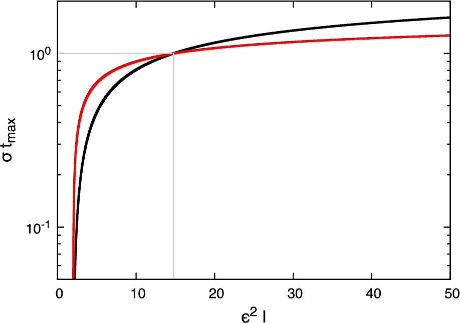
Maximal inverse Fourier time range at constant resolution width. For ϵ = 0.02 the value 10 on the x axis corresponds to 25 000 counts. The black curve is calculated from equation (20) implying a Lorentzian resolution, while the red curve is calculated from the generalised model with α = 2 (Gaussian resolution). The grey lines represent the situation where t max = 1 / σ .

It is also instructive to look at the situation of a fixed resolution represented by the grey vertical line in Fig. 1 representing σ = 1 . It can be seen that in this case an increase of the intensity by a factor of 10, e.g. by extending the registration time, only leads to a doubling of the maximal inverse Fourier time, but a reduction to 1/10 makes the data completely unreliable (on the level of ϵ = 0.02 ). Indeed, if one defines a dimensionless gain with respect to the naïve estimate for the maximal time for inverse Fourier transform, 1 / σ , as σ t max , then (20) σ t max = 1 2 ln ( ϵ 2 I 2 ) holds at constant σ (Fig. 2). Interestingly, this expression is independent of σ and allows to state that for a required accuracy of ϵ = 0.02 the ‘naïve estimate’ t max = 1 / σ holds at 2 e 2 / ϵ 2 ≈ 40000 counts. For I < 2 / ϵ 2 = 5000 , the S ( t ) from inverse Fourier transform becomes unreliable for all t. For I > 40000 the logarithmic increase of the accessible time range makes efforts to increase the flux or extending registration time cumbersome. Note that this calculation at constant σ did not make use of the specific form of I ( σ ) of this example. So the result can be considered general for instruments with a Lorentzian resolution function.

If one has the freedom to vary the resolution width, it is desirable to chose σ in a way that t max is maximised. A simple calculation yields the optimal resolution width (21) σ opt = 2 e ϵ I 1 and the achievable maximal inverse Fourier time for this choice: (22) t max , opt = ϵ I 1 2 e = 1 σ opt . It can be seen that if a flux increase is matched by a resolution narrowing σ ∝ I 1 one can obtain an increase of the accessible time range with the square root of the flux. Although this is not a dramatic increase it definitely surpasses the logarithmic increase at fixed σ.

Of course, in a real instrument a variety of resolution shapes is possible. The iconic counterexample to the Lorentzian would be the Gaussian, R ( ω ) = ( 1 / 2 π σ ) exp ( − ω 2 / 2 σ 2 ) 1

Similarly, the exponent 2 in (18) is too specific for the general situation. Therefore (18) is generalised to (24) I ( σ ) = I 1 σ β . As examples, β = 1 would correspond to the situation in a chopper time-of-flight instrument at constant incident wavelength where the number of neutrons is only reduced once in the primary spectrometer by narrowing the resolution at identical repeat rate. An addition of 1/2 to β would represent the situation where the resolution can only be improved by increasing the wavelength in the long-wavelength tail of a Maxwellian distribution I ( λ ) ∝ λ 4 .

OPEN IN VIEWER

Fig. 3.

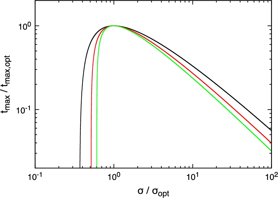
Maximal inverse Fourier time in the generalised model. t max and σ are scaled such that the maxima coincide. For this scaling, the values of β, I 1 and ϵ do not influence the shape of the curves. The values for α are 1 (green), 1.5 (red), and 2 (black).

The generalised model leads to a not much more complicated expression for the maximal inverse Fourier time, (25) t max = 1 σ ( ln ϵ + 1 2 ln I 1 + β 2 ln σ − 1 2 ln 2 ) 1 / α , and the optimal resolution width (26) σ opt = 2 1 / β e 1 / α ϵ 2 / β I 1 1 / β . The maximal inverse Fourier time achievable by optimising the resolution width is in that case (27) t max , opt = ( β / α ) 1 / α ϵ 2 / β I 1 1 / β 2 1 / α + 1 / β e 1 / α = ( β 2 α ) 1 / α 1 σ opt . Figure 3 shows the result of (25) rescaled to σ opt and t max , opt (which is a master curve with the only parameter α). Apart from being a bit narrower in general the curves for α > 1 are similar to those in Fig. 1. There is a strong cut-off on the side of too narrow resolution while there is a weak decrease ∼ σ − 1 ( ln σ ) 1 / α towards wide resolution.

The generalisation of (20) is (28) σ t max = ( 1 2 ln ( ϵ 2 I 2 ) ) 1 / α , and Fig. 2 also includes the calculation of σ t max for constant resolution width for a Gaussian resolution α = 2 . It can be seen that, compared to the Lorentzian resolution shape, the appearance is not much changed. Again, for counts larger than 2 e 2 / ϵ 2 there is not much gain in time range, here even only proportional to log I . The breakdown at low intensities is more pronounced but shifted, so that for a Gaussian resolution slightly deficient counts may be more tolerable.

Knowledge of the exponents α, β and the intensity factor I 1 would allow to calculate the optimal resolution width for the ‘generalised model’ of Section 4 for a required accuracy ϵ in S ( t ) from equation (26). Even if the shape of the resolution R ˆ ( x ) and the relation I ( σ ) are not those assumed in the preceding section it would still be possible to calculate the optimal resolution by determining the maximum of the general expression (15). But such detailed knowledge may only exist for a few instruments.

Nevertheless it is possible to derive a very simple criterion indicating whether a chosen resolution is too narrow or too wide. Replacing I 1 σ opt β by I ( σ opt ) in (26) and solving for the latter one obtains (29) I ( σ opt ) = 2 ϵ − 2 exp ( β / α ) . If the actual counts are larger than this value it is better to narrow the resolution, and in the opposite case it is better to widen it. The functional relation I ( σ ) is only important as it determines β. It could even be not a power law and (29) would still be applicable with β being the exponent of a locally approximating power law. This could also be determined in the course of the optimisation procedure. When two resolution widths are tried out a practical estimate is β = log ( I ( σ 2 ) / I ( σ 1 ) ) / log ( σ 2 / σ 1 ) . Since there are usually numerous resolution measurements existing for an instrument α should be well known.

In practice the instrument-dependent factor in (29) will be in the range exp ( 1 / 2 … 2 ) = 1.6 … 7.4 . So some knowledge of the exponents α and β will be necessary. But what is more important is that the accuracy requirement ϵ is correctly stated. For an expected intermediate scattering function S ( t ) spanning the whole range from one to zero, even an accuracy ϵ = 0.05 may be sufficient. On the other hand, for a large elastic incoherent structure factor a choice like 0.01 may be more appropriate. This gives a factor of 25 in the required counts which is much larger than what results from the uncertainty of the exponents α and β.

6. Discussion

The preceding sections show that the proviso of maximising the time range t max attained after inverse Fourier transform leads to a definite criterion for balancing resolution and intensity in QENS spectra. But it may be argued that this is only relevant if inverse Fourier transform is used as a data evaluation step in the investigation. This is nowadays often done, especially in cases where different QENS instruments have to be combined [11,13,15]. But in many studies the scattering function S ( ω ) itself is fitted by a model function f p ( ω ) where p is the set of parameters to be determined from the fit. This is usually done by minimising the integral square deviation (30) D ω ( p ) = ∫ | S ( ω ) − f p ( ω ) | 2 d ω . If the fit is performed on the inverse Fourier transformed data instead the quantity to be minimised is (31) D t ( p ) = ∫ | S ( t ) − f p ( t ) | 2 d t where f p ( t ) is the inverse Fourier transform of f p ( ω ) . According to Plancherel’s theorem [3] D ω ( p ) and D t ( p ) only differ by a constant factor.3

Another important aspect is the practicability of the procedure. If a full registration of a spectrum with subsequent inverse Fourier transform would be required to determine t max it would probably not be justified to do this only for the purpose of optimising the resolution. But the criterion presented here just requires the determination of the total count rate per detector in a short run. This allows the extrapolation to the expected count number in a full run which is required.

The change of resolution on a ToF-ToF spectrometer requires negligible time because only the chopper frequencies and phases have to be changed. On a crystal-ToF instrument usually the secondary instrument has to be moved which is a bit more time-consuming. But in both cases it will be justified to perform a couple of tests to optimise the resolution. Similarly on ‘inverted’ instruments [1,10] where the initial neutron energy is determined by time-of-flight and the energy after scattering selected by near-backscattering the resolution can be changed easily by the chopper phasing. The situation is different on exact backscattering spectrometers because there the resolution is fixed by the analyser crystals and their orientation. On the current backscattering instruments (and probably also in the future) changing the resolution requires a major dis- and reassembly. So the optimal resolution has to be determined beforehand from experiences on the instrument. Still, equation (20) may help to calculate the required and sensible measuring time from an initial measurement of the count rate.

It is shown that the maximal time t max which can be attained by inverse Fourier transform of QENS spectra establishes a criterion for the optimisation of the resolution on a QENS instrument. Equation (29) allows to decide whether the resolution can be improved at the expense of count rate or vice versa.

Alternatively, for a fixed resolution, it is possible to calculate the number of counts required from equation (28). Interestingly, the count number per detector to achieve t max = 1 / σ for the rather general model of Section 4 is fixed by the required accuracy ϵ only as 2 e 2 / ϵ 2 , which is ≈ 40000 for ϵ = 0.02 . From Fig. 2 it is clear that an increase of statistics beyond that number does not give a substantial improvement of the time range, while a reduction carries the danger of severe degradation.

Since the proposed criteria only use the total intensity per detector they can be easily checked in the beginning of an experiment. In an automatised experiment setting the determination of I ( σ ) could be done by an instrument control script beforehand and σ set to the optimal value for the subsequent experiment. Apart from the use when performing an experiment, the criteria may also be helpful in the design of future instruments since they allow a quick verification of the balance between resolution and intensity.