
Abstract
Road-object detection, recognition, and tracking are vital tasks that must be performed reliably and accurately by self-driving car systems in order to achieve the automation/autonomy goal. Other vehicles are one of the main objects that the egocar must accurately detect and track on the road. However, deep-learning approaches proved their effectiveness at the expense of very demanding computational power and low throughput. They must be deployed on expensive CPUs and GPUs. Thus, in this work, a lightweight vehicle detection and tracking technique (LWVDT) is suggested to fit low-cost CPUs without sacrificing robustness, speed, or comprehension. The LWVDT is suitable for deployment in both advanced driving assistance systems (ADAS) functions and autonomous-car subsystems. The implementation is a sequence of computer-vision techniques fused together and merged with machine-learning procedures to strengthen each other and streamline execution. The algorithm details and their execution are revealed in detail. The LWVDT processes raw RGB camera pictures to generate vehicle boundary boxes and tracks them from frame to frame. The performance of the proposed pipeline is assessed using real road camera images and video recordings under different circumstances and lighting/shading conditions. Moreover, it is also tested against the well-known KITTI database, achieving an average accuracy of 87%.
Keywords
Introduction
The main reasons for installing ADAS subsystems in current vehicles are to increase safety, decrease traffic accidents, and improve comfort and the driving experience [1, 2, 3]. Major automakers have started implementing a variety of high-tech ADAS features in recent years [4, 5] such as lane-departure warning (LDW), anti-lock braking system (ABS), electronic stability control (ESC) [6], lane-keep assist (LKA) [7], etc. These features signify slow but steady progress in the direction of a potential future with secure, completely autonomous cars [8, 9, 10, 11, 12].
The most recent ADAS features, such as collision warning, emergency braking, automated urban driving, autonomous highway driving (Autopilot), collaborative maneuvering, and automated parking are all examples of automated driving technologies, that call for increasingly quick and accurate finding and tracking of automobiles on roads [13], which is one of the very difficult and demanding tasks. These cars’ relative positions in relation to the motorway, the assessment and verification of the automobile’s movement direction, and the correct localization of possible automobiles in camera pictures or LiDAR data are necessary for successfully detecting the other vehicles on the road.
The primary instruments that enable the ability to understand the neighboring and distant environments for the tracking, identification, and detection of moving automobiles are thought to be computer vision techniques. Finding specific patterns, characteristics, or signals in images, like color distributions, colored segments, gradients, and edges, is the main constituent of the method that speeds up or directs the vehicle-detecting procedure.
The method utilized in this publication, called LWVDT which is a lightweight automobile finding and tracking, concentrates on a thoughtful balance between the three below-listed goals:
Precise on-road vehicle detection from pictures captured by the car’s camera mounted on the front windshield. Quick enough to enable the autonomous car to make fast and precise decisions and follow up with them. Avoid complicated architecture (e.g., manageable memory necessities and computing complexity) which can be implemented using inexpensive CPUs in real-time, such as those commonly used in ADAS building blocks.
Further, the methodology combines cutting-edge hand-crafted features that have been extracted from camera pictures along with a reliable classifier developed using machine-learning techniques in order to detect cars using cutting-edge hand-crafted features. This method accomplishes the coming objectives:
The extracted hand-crafted features can be combined and adjusted flexibly, as some of them can be integrated to create a so-called “feature vector”. Its adaptability enables some sort of color channels that has been selected from various color spaces to be included in the feature vector. Additionally, you can customize the LWVDT pipeline by setting a concise number of parameters. There is no need to reconstruct or design the entire process or entirely train the employed neural networks repetitively as with the techniques that depend on deep learning. Such adaptability also assists to adjust LWVDT for multiple higher or lower camera resolutions without significant loss of precision. Also, the transparent structure of LWVDT makes it much easier to extend and improve in the future compared to deep learning-based techniques that typically have a black-box arrangement. In this method, the sophisticated feature extraction stage is executed by inexpensive CPUs in a relatively short amount of time, and it does not require the involvement of GPUs in the process, which is common in approaches based on deep learning. The computational resources (in the form of memory requirements and computational power) required for LWVDT are significantly less than those required for deep learning algorithms. It is therefore more appropriate for ADAS subsystems running on classical scalar processors with thirty-two-bit architecture.
When it comes to in-vehicle finding and recognition, execution time is as crucial as accuracy. Instead of sacrificing runtime for accuracy, one needs to reach the balance between runtime and accuracy. The review below shows that the methods based on deep learning have achieved substantial success in automobile detection and have improved performance over classical approaches, but these methods are computationally intensive and, in most cases, expensive. However, they failed to deliver acceptable real-time performance, even with large GPUs and multi-core processors.
According to Wei et al. [14], convolutional neural network (CNN) feature maps may be enhanced with context and deeper features through the use of deconvolution and fusion techniques, improving object recognition and addressing occlusion issues. In order to evaluate the suggested CNN improvements, images with a resolution of 1280
In addition, Hu et al. [16] present SINet which is a CNN that is scale-independent for quick vehicle detection with widespread alterations. Those researchers also suggest that the detection precision is enhanced by employing context-aware region-of-interest (ROI) pooling in conjunction with multi-branch decision networks. Assessment experimentation was performed on Ubuntu 14.04 employing the KITTI dataset [15] and running on a sole NVIDIA-TITAN-X GPU in addition to eight CPUs (Intel(R) Xeon(R) E5-1620 ver3 at 3.5 GHz). Even though the use of very high-cost hardware, the stated inference time per frame is only 0.2 seconds, which corresponds to a speed of only five frames per second even with the use of very expensive hardware.
In his MSc thesis, Xiao uses advanced vehicle detection models to assist in the detection of vehicles [17]. A residual neural network can be used as a feature extractor in the model, and a region proposal network can be used to identify candidate ROI extractors. In this study, the main focus is on addressing the challenges associated with large-scale fluctuations so as to enhance automobile detectors’ performance. On a GTX 1080 GPU with 11 GB of RAM, the model was able to achieve 0.269 sec/frame for the inference task (i.e., lower than 3.7 FPS) with a GTX 1080 GPU.
Further recent work employs the CNN network to extract vehicle attributes [18], as they show robusteness and appropriate for a wide range of difficult circumstances [19]. Vehicle identification based on CNN, for instance, may be separated into two sub-categories [20]: one-stage or two-stage vehicle detection approaches [21]. One-stage vehicle detection approaches, such as RetinaNet [22], CFENet [23], CornerNet [24], YOL [25], SSD [26], and others, may pass the original picture straight into the CNN model for vehicle feature extraction and receive the vehicle’s position and category via regression and classification. Moreover, Cascade R-CNN [27], Faster R-CNN [28], Mask RCNN [29], R-FCN [30], and SPP-Net [31] are two-stage vehicle detection algorithms that identify potential vehicle areas in the picture and then feed them into the CNN model for feature extraction and classification. When compared to two-stage vehicle identification systems, one-stage vehicle detection methods save time and are less expensive. However, the accuracy of these approaches’ vehicle classification is rather poor since they only conduct the object localization and classification tasks on an input picture once with a single neural network [18].
As a result of this work, the following contributions have been achieved:
Execution in Real-time: There are several advantages to the proposed pipeline, including the fact that it focuses on enabling the deployment of ADAS object detection capabilities as soon as possible on low-cost automotive hardware. The goal is to reach 10 FPS [32] and avoid the employment of GPUs. The throughput does not rely on iterative searches, it relies on one scan per camera image. This is a result of using an efficient method to focus computations on picture sectors of high importance. Incorporation of numerous color spaces: In this study, the authors use compound color spaces to increase the strength of extracting features and combine them into a further all-inclusive “feature vector”. The employed classifier has been trained in several color spaces. Adaptability and Flexibility: The LWVDT algorithm can be customized by tuning only a small count of parameters. There is no need to reconstruct and design the entire process or entirely train the employed neural networks repetitively as is the case with techniques based on deep learning. Such manipulability also facilitates the adjustment of LWVDT for lower or higher multiple resolutions of the camera with no significant shortfall of precision. LWVDT also has a transparent structure, which makes future extensions and improvements much easier than deep learning-based techniques, which typically have a black-box arrangement. Reusability: The suggested procedure has the capability to be employed multiple times with few changes to recognize more objects on the motorway, such as bikes, pedestrians, traffic lights, and road signs.
The LWVDT execution process.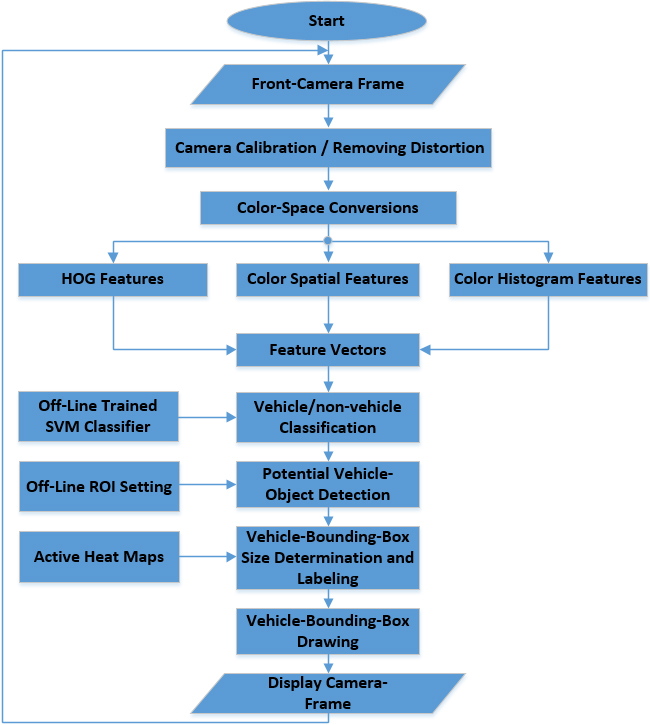
The LWVDT pipeline is constructed to use a sole charge-coupled device video camera (CCD). Such a video camera ought to be fixed on the car’s front windshield mirror to capture the front view of the motorway. Nevertheless, stereo cameras are also applicable, but for the sake of simplicity, only a front sole camera is considered in this work. To streamline the problem of detection, the authors knowledgeably assume that the baseline is a perfect horizontal line due to the setting. This ensures that the “horizon line” is in the picture and the X-axis is parallel to it (i.e. the intersection of the right and left lane lines is projected in a plane called “Horizon” and it is determined using one of the methods explained in [33]). However, for the sake of accuracy, LWVDT uses the front camera calibration data to orient the image and remove visual distortion. The following steps in addition to Fig. 1 provide an overview of the overall procedure and clarify the combination and collaboration of the technologies used:
Calibration of the Camera: The supplied color picture to the LWVDT pipeline is supposed to be an RGB 1200x720 in size. Then, the algorithm initially removes the distortion and adjusts the alignment using the checkerboard image camera calibration method. This camera calibration method is performed merely once when the LWVDT algorithm is initialized, instead of every iteration/frame, therefore, it does not affect the real-time functionality. Conversion of Color spaces: The calibrated picture is then transformed to grayscale and multiple color spaces [34] (YCrCb, HSL, LAB, HSV, YUV, LUV, etc. [35]). Each color space has its own unique characteristics that increase LWVDT performance. Not all of these color spaces are included in the final LWVDT pipeline. The final pipeline has been established and will be detailed later, and discussed in more detail in a later section of this study. Some of such color space transformations are done through research, analysis, testing, and trial-and-error to reach that goal.
Identified automobile boundary by the LWVDT technique.
Identified automobiles’ boundaries by the LWVDT technique. Extraction of Features: Once the color and grayscale space transformation steps got carried out, numerous features are extracted from the calibrated camera image, such as the histogram of orientation gradients (HOG) [35], color space/spatial properties [36], and color histogram properties [37]. How those features are extracted is detailed in the next section. Those properties (features) are then assimilated to create a long vector given the name “feature vector”. Classification into vehicles or not: Those feature vectors are then supplied to a classifier that separates vehicle and non-vehicle images. The support vector machine (SVM) classifier is constructed, employed, and trained offline [38] to recognize feature vectors that represent vehicles and those that do not (the ones that represent vehicles will move on to the next step). Full creation and learning of the SVM classifier are detailed in the coming sections (no. 6). Possible automobile object finding: Afterwards, the vehicle images are separated from non-vehicle images by classifying the feature vectors, prospective automobile entities in the camera pictures are found by means of a combination of SVM classifier and sliding windows, and the calibrated camera pictures are scanned to find and identify these automobile objects [39]. Scans are not performed on fully calibrated camera images, but the ROI are identified and separated from each picture to execute this comprehensive search in it [40, 41] with the lowest computational load. Therefore, unwanted picture details are masked to accelerate vehicle boundary finding, enrich the concentration and precision of the finding process, and produce potentially accurate car boxes. Sizing and labeling of vehicle bounding boxes: The outcome of the previous scanning process is employed to create an active heatmap that gathers potential automobile boxes. The duplicated or overlapped true-positive automobile boxes are gathered into larger boxes and marked correspondingly. Automobile bounding boxes drawing: In the step that terminates the process, marked boxes are sketched on the primary camera or frame image. In favor of demonstration purposes, real-life examples of the resulting street boundaries are depicted over the primary color picture, as shown in Figs 2 and 3.
The HOG feature descriptor is used in image processing and computer vision for the purpose of recognizing and detecting objects in images and video [42]. As an example, to find a definite object ‘
The camera picture is transformed into a grayscale. Initially, create a rectangular (or squared) window with a size of 64 pixels high and 64 pixels wide (those dimensions of the created window can be selected arbitrarily, and be determined by the designer’s selection). Employ it to examine the gray camera picture and search for ‘ Of course, the object With the sliding of the window, at each step, HOG features are calculated and linked to the corresponding window center location for “feature localization”.
Workflow of the histogram of oriented gradients.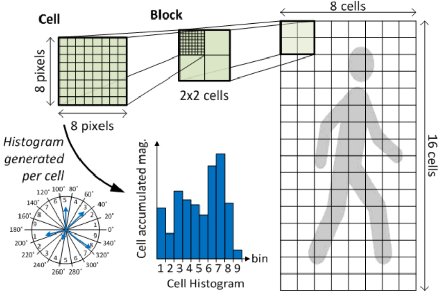
In order to calculate the HOG features, the entry point to the technique is assumed to be a specific window ‘
where the row and column counts of pixels are The computed slope (e.g. gradient) is transformed to polar coordinates and the angle is restrained from 0∘ to 180∘ as follows: Consequently, the gradient pointing in the opposite direction is computed as
where By the division of the window
and the vote:
Such a format is named voting by bilinear interpolation. Moreover, the resultant cell histogram is a vector with A block normalization phase is afterward performed by assembling the cells into overlapping blocks of 2
where The block features that have been normalized are then glued together into a vector
where
HOG applied to images and showing results.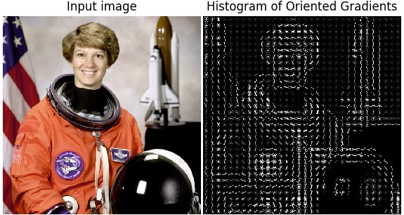
A supervised training model called the Support Vector Machine (SVM) [38] analyzes data used in regression and classification analysis [43]. An SVM training algorithm creates a model that categorizes new examples corresponding to one of two categories given a set of training examples that have each been denoted as belonging to one of the categories. By doing this, the technique can be described as a binary linear classifier which is non-probabilistic.
Given
where
Any hyperplane can be expressed as the collection of
where
The optimization objective function can be expressed as follows if the training data can be separated linearly:
Our classifier,
The hinge loss function is introduced as follows if the training data cannot be linearly separated:
If the constraint
where the parameter
If a classification law that is nonlinear must be obtained, and if the converted data points
where solving the following optimization problem yields the
Quadratic programming can be used to solve the coefficients
Last but not least, new points (
A camera’s display of a 3-D actual scene converts it to a 2-D one, however, the translation from three-dimensional to two-dimensional is not flawless, leading to image distortion. Actually, compared to their 3D appearance, objects’ sizes and shapes are deformed (altered) in the final 2D image. Thus, this distortion needs to be corrected before employing the resulting 2D camera pictures in order to extract and evaluate the accurate and usable information.
Real cameras are built with curved lenses that produce a picture. Depending on the focus and positioning of the objects, the light normally bends to a low or high degree along the borders of these lenses. As a result, there is distortion along the margins of the images, making straight lines or bodies appear to be more or less rounded than they actually are. The main source of deformation is this phenomenon, which is known as “radial distortion”.
Furthermore, “tangential distortion” is a significant source of distortion. When the lens of the camera is not completely aligned with the picture plane that is related to the camera sensor and parallel to it, distortion occurs. This causes the image to tilt, making objects appear closer or farther away than they are.
To correct for radial distortion, three coefficients are required:
Pictures with distorted and undistorted (corrected) points.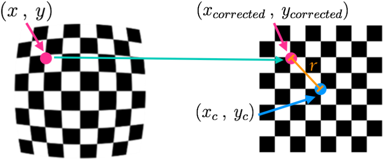
Mapping from a distorted chessboard image to an undistorted one.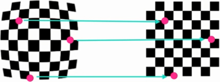
Calibration pictures of chessboards with corners sketched.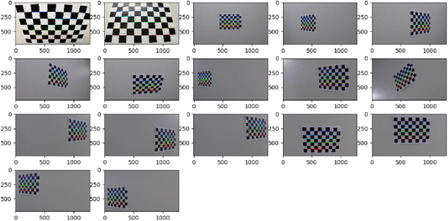
In Eqs (19) and (20), (
Tangential distortion is accounted for by two additional coefficients:
Pictures of known shapes (chessboard pictures) are employed to correct for the aforementioned distortions. As shown in Fig. 7, designated pixels in the deformed plans are afterward mapped to undeformed plans. Consequently, the images from the camera will be calibrated. To improve image quality and undistort captured camera images, the following procedure is used:
Step 1: Locate the chessboard corners: The “cv2.findChessboardCorners()” procedure from the OpenCv3 package [44] is employed to find the chessboard corners by means of 20 chessboard pictures of varying sizes and orientations, as shown in Fig. 8. The detected number of corners is 9 Step 2: Obtain camera matrices: To find the camera matrices, an experiment chessboard picture that has not previously been employed in detecting the corners is employed, shadowing being transformed to greyscale, along with the detected corners in the first step. This is done with the “cv2.CalibrateCamera()” function. To examine the calibration worthiness, use the grey testing picture along with the camera matrices to eliminate the deformation from this picture, as displayed in Fig. 9.
A testing picture of a chessboard with deformation removed. Step 3: Camera matrices saving: Employing the Pickle software package [45], the camera data (camera specs matrix and distortion coefficients) are stored in the pickle file “camera calibration.p” to be recovered later.
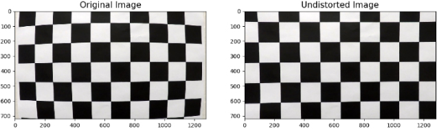
Figure 10 shows how to apply the camera calibration technique to one of the testing pictures.
The influence of camera calibration (removing distortion of pictures).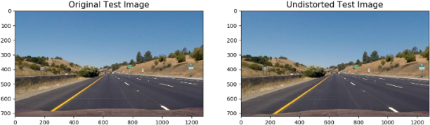
In this part, the methods to develop a classifier based on the SVM machine learning technique mentioned in Section 4 will be described here in detail, while it will be given the acronym “SVMC”.
Preparation of the training data
The following summarizes the data preparation stages for training the SVMC:
Udacity-supplied data [46, 47]: Udacity-supplied data were used during the course of this investigation. The data comprises almost equalized pictures of “non-vehicles” and “vehicles”:
The “non-vehicle” assortments are the “GTI” [48] and “Extras” collections. Each has 8,968 RGB pictures with sizes of (64, 64, 3) pixels. The “vehicles” assortments comprise the “GTI” and “KITTI”. Each has 8,792 RGB pictures with sizes of (64, 64, 3) pixels. These assortments are 149MB in size when unzipped. Augmentation of the Data: All of the images are flipped around the “Y” axis to enrich the data. As a consequence, the training data grew to 35,520 pictures.
In the sequence of execution, the following phases explain the implemented data visualization steps:
50 automobile pictures visualization (chosen randomly).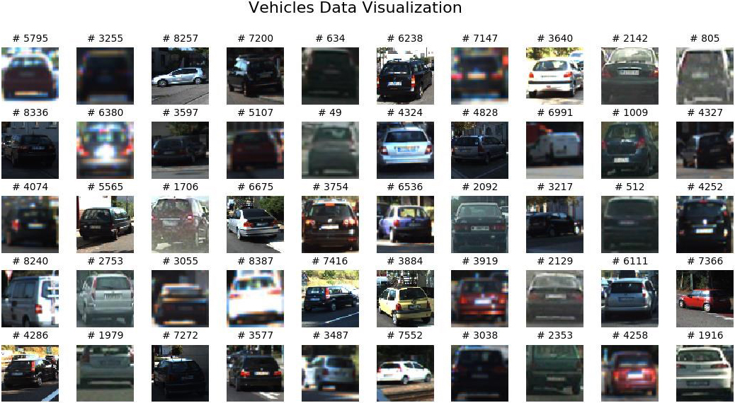
50 non-automobile pictures visualization (chosen randomly).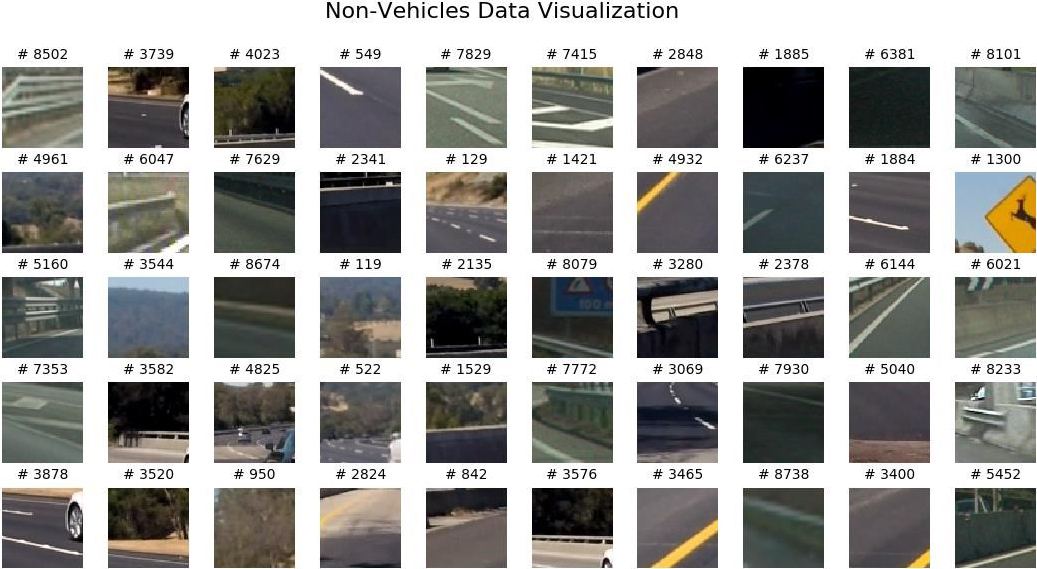
HOG feature visualization for car and non-car images.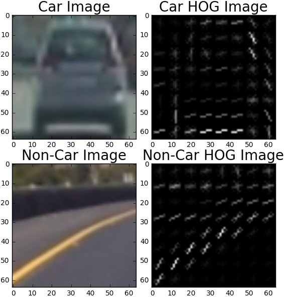
Feature vector visualization for vehicle pictures.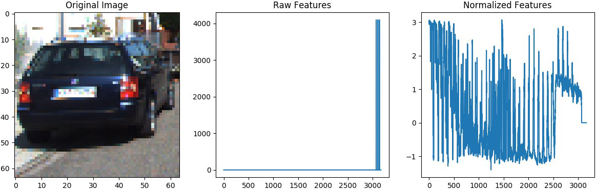
Vehicle Data Display: As illustrated in Fig. 11, 50 pictures selected at random of automobile data have been presented. Each image has a title that corresponds to its position in the training data. Non-Vehicle Data Display: As shown in Fig. 12, 50 pictures selected at random of non-automobile data have been presented. Each image has a title that corresponds to its position in the training data. Presentation of HOG features of Vehicle Data: After converting the picture to grayscale, a selected picture of the automobile data was utilized to extract its hog characteristics. Furthermore, the HOG aspects of non-car cases are obtained, and the results are displayed in Fig. 13.
In the sequence of execution, the following stages explain the realized picture feature extraction procedures:
Features of Color Spatial: A method is built to obtain the influence of each image’s distinct color channels. To compute the binned color characteristics, in other words. Each image’s channel is scaled to (32 Features of Color Histogram: A procedure is provided to calculate the histogram of each color channel in each picture using a specified count of pins, and afterward glue them together. Computing HOG Properties: A procedure is created to calculate the HOG quantities of each picture channel individually, which may afterward be used independently or appended collectively if this option is chosen. In this example, the SciKit-Image procedure “hog” [49] is utilized. Integrating Everything: The following feature vectors are produced by the aforesaid feature extraction functions:
Utilizing color spatial features and “spatial size Utilizing color histogram features and “histogram bins Applying the HOG extracted quantities and the values “gradient orientations cells If all of the aforementioned procedures are employed, the final feature vector will have 3,072
The procedures below are employed to construct the SVMC classifier that separates vehicle images from non-vehicle images and train it:
Creating a 35,520 Before joining the feature datasets, they should be scaled using the SciKit-Learn “StandardScaler().fit()” algorithm [50]. The display of unrefined and normalized feature vectors for an automobile picture is shown in Fig. 14. Creating an output training set “Y” of 35,520 Using the SciKit-Learn “train test split()” method, the training datasets must be randomly shuffled and divided into 20% for validation and 80% for learning. Employing the SciKit-Learn library’s Linear Space Vector Machine Classifier function “LinearSVC()” [51], the constructed classifier was trained with good precision (above 97.7%) in practically all parameter combinations. The trained model is then put to the test on the provided test pictures. In some situations, the outcomes were poor. Extensive experiments were carried out with several parameter combinations, nevertheless, the outcomes were still unacceptable. Following multiple tries and mistakes, it is discovered that the color spatial characteristics consume a substantial percentage of the feature vector span ( The updated Linear SVC classifier is built using various color spaces and a training dataset with a size of 35,520 With the exception of “RGB”, almost other color spaces yielded equivalent results. The “LAB” color space outperforms the “YUV” color space in both learning and prediction, with the 2nd place in the precision results. Nevertheless, when tested on test photos, “YUV” yielded more false positives than “LAB”. As a result, the “LAB” color space is chosen for the coming phases. The SVC learning duration has no effect on the functioning of the LWVDT algorithm since it is executed offline; nevertheless, the label prediction time has an effect on the performance because it is included in the finding time for each camera frame.
Linear SVC training results
The below-listed stages set up the procedure (LWVDT) employed in the finding and tracking of the driving automobiles other than the egocar on the motorway. The following steps are stated here in the same order which will be executed:
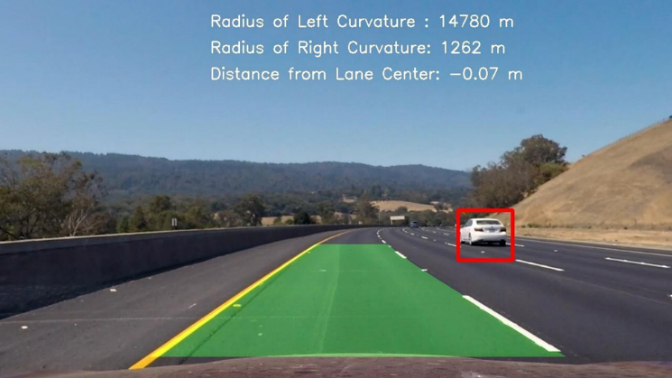
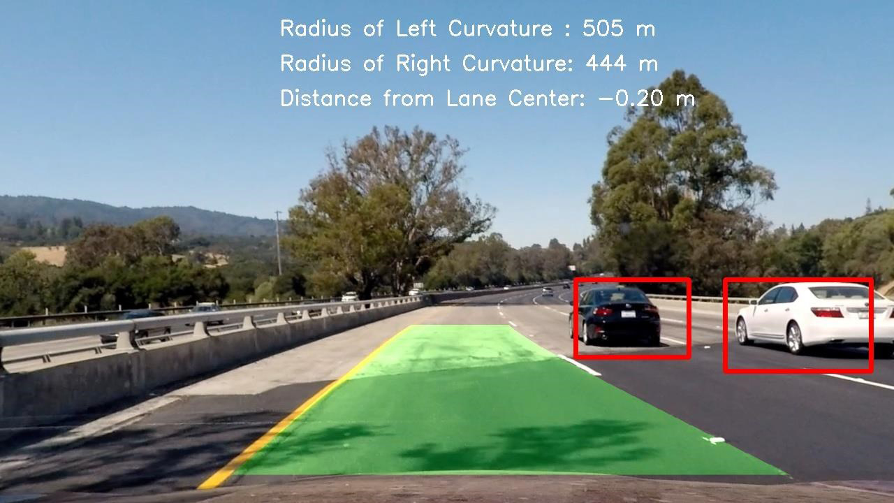
Detection of Lane boundaries: this procedure is primarily to find the street borderlines (i.e. the lane lines in front of the automobile) which denote the front drivable area (exhibited in green in Fig. 2). This procedure is fully realized in [52] and employed in this text for suitability. Identifying automobiles using the sliding windows technique: for each camera frame, a specialized function is constructed and invoked, using the below factors and limits:
“orient “pix per cell “cell per block
“step size “Scale Step Scale_Multiplier_Start, Scale_Multiplier_End: a couple of parameters that define when the window sizes slowly increase while inspecting the ROI region. The procedure applies the taught developed SVMC classifier to every built search window. Figure 15 depicts the construction of sliding windows of various sizes to cover the required ROI. This function may be repeated numerous times with a new set of “a Active heatmaps Creation: The purpose is to create a heatmap for each detected automobile box for the duration of a sliding-windows scan search. This heatmap is employed to separate (or at least reduce) the number of false-positive boxes. As illustrated in Fig. 16, a specific boundary “HEAT_THRESHOLD” is utilized to merely pass (depending on its assigned amount) the automobile boxes with numerous impacts (true-positive boxes). Car boxes labeling: the overlapped true-positive automobile boxes are afterward aggregated into larger boxes and labeled with the Sci-Kit Learn library’s “label()” method. Creating the labeled automobile boxes: Finally, the labeled boxes are sketched on the primary validation picture or frame of a video, as illustrated in Figs 2 and 3.
Figures 17 and 18 illustrate instances of the findings obtained after running the aforesaid algorithm on the validation pictures, which contain shadow patterns that typically mislead vision-based techniques.
Sliding panes of varying sizes scan the ROI.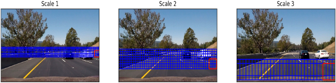
Computing throughput for the LWVDT pipeline
Found automobile boxes and the resulting heatmaps.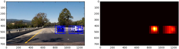
The proposed LWVDT method is then tested on several images reflecting various scenarios. The outcomes reveal that the pipeline operates admirably under various scenarios (at sunset, at full sunrise, without shadows, with shadows, with no vehicles on the adjacent lanes, and with automobiles on the adjacent lanes). Additionally, for healthiness testing and validation of the created algorithm, the pipeline is applied to many real-time video instances reflecting various driving scenarios. The LWVDT proved to be quite robust in all of the preceding situations, as illustrated in Figs 2 and 3. Yet, as demonstrated in Figs 17 and 18, the scattered portions of shadows influence the accuracy of constructing the automobiles’ border boxes. Yet, the findings are still good enough and create effective working output.
Figures 2, 3, 17, and 18 demonstrate the lane detection findings applied in the work of [7, 39] alongside the vehicle detection results of this paper.
In real-time execution, the pipeline proved to be acceptable. The below-listed quantities are measured for a couple of investigating video records using an Intel dual-core with 8GB RAM Core i5-4200U at 1.6 GHz, which is a pretty reasonable computational platform.
Automobile identification and tracking pipeline execution.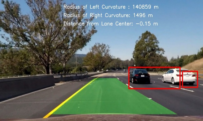
Automobile identification and tracking pipeline execution.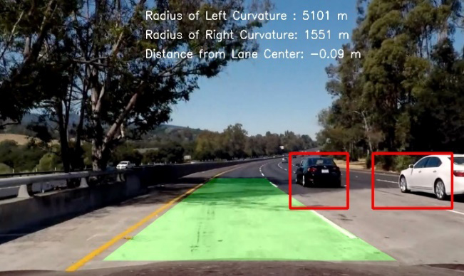
The slowest recorded sorting-out throughput is 10.01 FPS. This is believed to be appropriate for this application’s desired performance [32]. As a result, using more powerful processing gear should greatly improve the real-time outcome of the suggested procedure.
The experimental findings are evaluated for LWVDT performance using the three statistical measures test of a binary classification [53]: Precision, Recall, and Intersection over Union (IoU). The fraction of actual positive samples to all positively recognized samples indicates how accurate the forecasts are. The proportion of actual positive samples that are accurately identified is measured by recall (e.g., the percentage of automobile pictures, which are recognized as true automobile pictures). The IoU metric calculates the overlapping percentage between the predicted and ground-truth areas to determine how reliable our detector is in comparison to the ground truth. Such expressions are as follows:
where TP designates the count of true positives; in other words, the count of correctly identified vehicle pictures; The count of true negatives (TN) is the count of accurately categorized non-vehicle pictures. The count of false positives is denoted by FP. the count of photos of vehicles classed as non-automobile; The count of false negatives (FN) is the count of non-automobile pictures sorted out as vehicles.
The well-known average precision (AP) and intersection over union (IoU) metrics [53], which have been extensively employed to evaluate numerous automobile recognition techniques, are employed here to assess and compare the functioning of our proposed LWVDT to up-to-date methodologies [54, 55, 56]. The Single-Shot Detector (SSD) [54] is a cutting-edge single-stage detector that produces predictions by leveraging different feature map resolutions. Another sort of single-stage detector is You Only Look Once (YOLO) [55], which produces predictions by seeing unrefined picture information as a 7
Table 3 evaluates the suggested LWVDT method against the up-to-date deep-learning-based techniques (e.g., Fast R-CNN, SSD, and YOLO), using the KITTI dataset [14]. The deeplearning methods clearly outperform the LWVDT in terms of detection accuracy, but at the penalty of massive computing expense. For instance, YOLOv2 has a high mean precision (AP) as well as real-time functioning on an expensive GPU (37 FPS). Unfortunately, performance on a very high-end CPU is very low (0.08 FPS), if we compare it to the 12.52 FPS of the LWVDT on a low-end reasonably-priced CPU. For ADAS systems with comparatively low computational resources, the feature development and deployment cost are as critical as precision, and the car industry requires a fine balance between the two.
Comparison of various algorithms on the KITTI vehicle-detection validation dataset
The LWVDT pipeline is also executed on the cloud platform: Google Colab [58] using a couple of modes: GPU (NVIDIA Tesla K80, 13GB RAM) and TPU (v2) [58]. The top values obtained on the GPU are 0.058 seconds while on the TPU is 0.073 seconds. These tests show that there isn’t much of a difference in performance when compared to CPU findings. The GPU contributed only a 27% increase in computing performance, and in the meantime, the TPU contributed merely 7.5%. The reason behind such an outcome is that the GPU is mostly used to accelerate matrix computations, and the built algorithm includes a lot of matrix calculations. Furthermore, the TPU is primarily intended to accelerate tensor-based computations, which are not employed in the formulation of the RT VDT algorithm. The RT VDT algorithm’s performance is also depicted in Figs 19 and 20 below.
Identified automobile boundary by the LWVDT methodology on the KITTI dataset-1.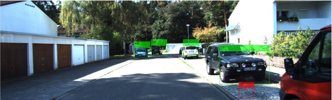
Identified automobile boundary using the LWVDT methodology on the KITTI dataset-2.
The below viewpoints throw more light on various technical methods and properties tried or carried out in the previously explained pipelines:
Decision function: As an alternative to a simple estimation function, the decision procedure [50] (from the SciKit-Learn module) is utilized after applying the accomplished SVMC prototype to each built sliding window to hunt for automobiles. The judgment procedure outputs the likelihood that the object is an automobile or not. Positive probability indicates that the identified object is at least 50% an automobile, whereas negative probabilities indicate that the thing is higher than 50% non-car. Via creating a first-hand constraint “Confidence score”, that specifies an object’s trust in being an automobile. The greater the positive quantity, the greater the confidence in the thing being an automobile. The use of a decision function dramatically reduced false positives. Filtering heatmaps: the calculated heatmaps on each frame are not used directly, but are filtered using an FIR filter. Before applying a threshold, this FIR is meant to employ the current and earlier values of the preceding four frames. This procedure assisted in smoothing out the manufactured automobile windows as well as eliminating false positives. Filtering of the Vehicle box vertices: Like heatmaps, FIRs are used to filter out the constructed vehicle boxes. The generated vertices are not immediately used; rather, they are filtered employing the computed quantities of the three preceding frames. Such a strategy significantly facilitated to diminishing of the jitter of the detected final vehicle boxes’ location and size for each frame. Regions of interest identification: the LWVDT algorithm has been designed to incorporate the identification of various ROI inspecting areas by both the Down-sampling of frames count: During the course of the carrying-out tests, it was discovered that it is not essential to search for automobiles in every frame at the camera’s current sample rate (25 FPS), because vehicle movement between frames is very slow. As a result, the in-force search for automobiles is limited to every other frame, which cuts the video sorting out time in half and has almost little effect on the outcome. Sanity checks: Certain sanity checks, for example, are employed to enhance the indicated/detected car boxes, such as:
Size of the vehicle box: The detected vehicle box size is computed and confirmed before being sketched on the picture or video frame. This is accomplished by gauging the designated box’s diagonal and comparing it to certain limitations. Position of the vehicle box: various validation checks are introduced to confirm the location of the indicated automobile boxes. In the testing pictures, for example, vehicle boxes cannot be found below “y Color spaces: Approximately seven distinct color spaces have been tested on both test pictures and films. During the course of the investigation, both LAB and HSV delivered the greatest results in terms of automobile detection and false positives. Several color spaces, such as HLS, YCrCb, YUV, and LUV, provide equivalent results. RGB, on the other hand, generated by far the worst outcomes. As a result, during the implementation and validation phases, HSV and LAB are used.
Upon the completion of the vehicle tracking functionality. The natural continuation of this study will be to use visual, lidar, radar, and heuristic strategies to solve object detection, localization, navigation, path planning, and stability challenges.
Thorough out this work, a trustworthy and refined automobile identification and tracking system centered around hand-crafted feature extraction techniques is proposed and referred to as LWVDT. LWVDT employs a pipeline that includes well-established color spaces like LUV, YUV, LAB, and others. Furthermore, it employs computer-vision methods such as HOG features as well as machine-learning techniques such as Support Vector Machines. Furthermore, the proposed procedure employs extensive picture deformation suppression and camera calibration methods to generate undeformed street pictures appropriate for more precise automobile findings. Furthermore, many sanity-check approaches are utilized to strengthen the reliability of the employed methodologies. The suggested LWVDT approach requires just unrefined RGB pictures from a sole CCD camera located behind the vehicle’s forward-facing windscreen. The LWVDT algorithm’s functioning is validated and assessed utilizing a large number of stationary pictures and several real-time recorded videos. The assessment findings reveal that the detection is fairly accurate and resilient, with only a minor inconsequential divergence in one situation with complicated shadow patterns. The observed performance (running time) utilizing a low-cost CPU demonstrated that the LWVDT is well-suited for real-time vehicle detection even without the addition of additional processing capacity such as GPUs. Additionally, on the KITTI dataset, the functioning of the LWVDT pipeline is compared to that of the most recent deeplearning techniques. Deeplearning methods outperform LWVDT in terms of performance, but at a far larger computing cost (fairly expensive GPUs). For low-end Processors, however, the LWVDT real-time functioning confidently demonstrates that it is suitable for ADAS tasks or autonomous automobiles. Future research will concentrate on improving the algorithm’s detection and tracking of people and bikers.