An updated analysis of the predictive ability of Mexico’s Manufacturing Business Opinion Survey 1

Abstract

We present an analysis of the Manufacturing Business Opinion Survey carried out by Mexico’s national statistical agency. We describe first the survey and employ exploratory statistical analyses based on coincidences and cross-correlations. We also consider forecasting models for the indices of industrial production and the Mexican global economic activity, including opinion indicators as predictors as well as lags of the quantitative variable to be predicted, so that the net contribution of the opinion indicators can be best appreciated in a forecasting experiment. The forecasting models employed are statistically adequate in the sense that they satisfy the underlying assumptions, so that statistical inferences and conclusions are validated by the data at hand. Our results lend empirical support to the intuition that this survey provides information that anticipates the behavior of important macroeconomic variables, such as the Mexican index of global economic activity and the index of industrial production. We include a section where some original tables and figures covering data up to year 2009 are updated to include data up to October 2017. These new tables show that the original conclusions remain valid even though the data were subjected in 2011 to some modifications due to a three-fold increase of the sample size and an extended coverage of economic activities.

Keywords

Coincidences cross-correlation diffusion indices forecasting models macroeconomic prediction opinion indicators

1. Introduction

Economic agents tend to make rational decisions based on the largest amount of available information. Such information could be based on opinions and expectations from producers about the behavior of relevant variables of the economic system. On the basis of this belief and the assumption that the responses to opinion surveys provide reliable information, it makes sense to aggregate such responses to get an index of the behavior of such variables as production and global economic activity. This is the basic idea behind the calculation of diffusion indices, as defined by the manual of the Organisation for Economic Co-operation and Development (OECD), see [13, Section 5]. The information provided by the respondents are qualitative since they simply answer “Higher”, “Equal” or “Lower” to questions related to, for instance, production in a month relative to the previous one. Those answers are used to calculate quantitative indices that summarize the trend of a group of variables and that supposedly anticipate the behavior of relevant macroeconomic variables in the short run. At the international level, there are several studies that validate such an assumption, e.g., [1, 2, 3, 4, 5, 10, 15]. In this work, we aim at validating that assumption for Mexico, with data from the monthly Manufacturing Business Opinion Survey (MBOS).

The advantage of a business opinion survey is that it generates timely information that may prove useful in short term forecasting. The official Mexican statistical agency (INEGI) calculates several indices from the MBOS; two of the most important are the Aggregate Tendency Index (ATI) and the Manufacturing Orders Index (MOI). Here, we want to answer the question of whether the ATI and/or the MOI anticipate the monthly figure of industrial production and that of the Mexican Index of Global Economic Activity (IGEA). The latter index achieves almost 90% coverage of the quarterly Mexican Gross Domestic Product (GDP) and its figure is released 57 days after the end of the month of reference, while the GDP figure is published 52 days after the quarter of reference.

The following section describes the MBOS and the two main indices used in this work. Section 3 presents an exploratory analysis aimed basically at detecting potential relationships between qualitative variables from the survey and quantitative macroeconomic variables. Section 4 complements the previous analysis by using some quantitative data provided by the MBOS, even though such data are not true measurements but numerical opinions expressed by the respondents as quantitative beliefs. The fact that the MBOS provides this kind of data makes it different from similar opinion surveys and enriches the present analysis. This kind of information can be gathered by the MBOS because the National Law of Statistics [11] establishes as a legal duty that respondents must answer the questionnaires required by INEGI. Section 5 describes a forecasting experiment and shows the models employed to predict some relevant quantitative variables that incorporate the timely opinion indicators as predictors. The experiment was carried out to select the best models and validate their predictive ability with data for years 2009 and 2010. The last section concludes and makes some recommendations about the usage of the techniques and models employed.

2. Monthly manufacturing business opinion survey

The MBOS follows the OECD recommenda-tions [13]. Details on the sampling design and some other technicalities of the MBOS can be found in [12]. The summary of answers to questions that ask for an assessment of the change of one month with respect to the previous one is expressed in differences. Such is the case for most questions of the MBOS questionnaire, for instance, the question For the indicated periods, how was the volume of production of your firm? admits one of the following answers: Much higher, Higher, Equal, Lower and Much lower.

The opinion indices obtained from the MBOS are supposed to anticipate the economic facts, because the producers express expectations that tend to become plans, whose realizations are registered at the end as facts that can be measured with traditional quantitative surveys. The diffusion indices summarize the responses and assign weights in accordance to the firm’s relative importance, i.e. sales, fixed assets or occupied personnel of the firm, depending on the variable under consideration. The response combination leading to the respective index makes use of the following weights: 1.00 for Much higher or Much better; 0.75 for Higher or Better; 0.50 for Equal; 0.25 for Lower or Worse; and 0.00 for Much lower or Much worse. The central value is 0.5, which is considered the borderline between expansion of manufacturing activities (above 0.5) and contraction (below 0.5), although we should keep in mind that the weights are assigned arbitrarily.

We concentrate on ATI referred to the historical (previous month) behavior of the firm and MOI referred to its expected (current) behavior. The ATI combines data from five questions: Volume of Production; Use of Plant and Equipment; Domestic Demand; Volume of Exports; and Occupied Personnel. Responses to each question lead to obtaining the corresponding tendency subindices: Production (PROTI); Plant and Equipment (UPETI); Demand (DEMTI); Exports (EXPTI); and Occupied Personnel (OCPTI). To calculate these subindices in month t, the following percentage of responses are obtained, for each question and option $j=$ 1, $\ldots$ , 5,

$\displaystyle\text{Perc}(j)_{t}=\frac{\sum_{i=1}^{n}d_{jit}p_{i}f_{i}}{\sum_{i% =1}^{n}p_{i}f_{i}}\times 100,$ (1)

where $n$ is the number of firms in the sample, $p_{i}$ is the weight assigned to firm $i$ , $f_{i}$ is its expansion factor (the reciprocal of its probability of inclusion in the sample) and a dummy variable is used to indicate the response, i.e. it takes on the value $d_{jit}=$ 1if the answer of firm $i$ is $j$ and $d_{jit}=$ 0 otherwise. The weight $p_{i}$ for PROTI, DEMTI and EXPTI is sales volume, for UPETI is fixed asset and for OCPTI is occupied personnel. Each subindex is obtained as the linear combination

$\displaystyle Z_{t}=\sum_{j=1}^{5}w_{j}\text{Perc}(j)_{t},$ (2)

with $Z_{t}$ denoting PROTI ${}_{t}$ , UPETI ${}_{t}$ , DEMTI ${}_{t}$ , EXPTI ${}_{t}$ and OCPTI ${}_{t}$ , respectively, where the weights are $w_{1}=$ 1.00, $w_{2}=$ 0.75, $w_{3}=$ 0.50, $w_{4}=$ 0.25 and $w_{5}=$ 0.00. Finally, ATI is obtained as:

$\displaystyle\text{ATI}_{t}=(\text{PROTI}_{t}+\text{UPETI}_{t}+\text{DEMTI}_{t% }+\text{EXPTI}_{t}+\text{OCPTI}_{t})/5.$ (3)

MOI is derived from expectations of the producers about such variables as: Orders; Production; Occupied Personnel; Timely Supply Delivery; and level of Supply Inventory. The subindices generated are: Volume of Orders (VOMOI); Volume of Production (VPMOI); Occupied Personnel (OPMOI); Supply Delivery (SDMOI); and Supply Inventory (SIMOI). The percentages of responses are weighted as with the ATI except for SDMOI that is weighted as: Much faster, 0.00; Faster, 0.25; Equal, 0.50; Slower, 0.75; and Much slower, 1.00. Again, calculation of weighted percentages is done as in Eqs (1) and (2) where now $Z_{t}$ denotes VOMOI ${}_{t}$ , VPMOI ${}_{t}$ , OPMOI ${}_{t}$ , SDMOI ${}_{t}$ and SIMOI ${}_{t}$ . The weight for the percentages is sales volume, except for OPMOI which is weighted by occupied personnel. The final calculation applies another weighting to the components that reflects the stage of the productive process that is normally followed by manufacturing firms, that is: orders, 0.30; production, 0.25; occupied personnel, 0.20; supply delivery, 0.15; and supply inventory, 0.10. The weighted index becomes:

$\displaystyle\text{MOI}_{t}=0.3(\text{VOMOI}_{t})+0.25(\text{VPMOI}_{t})+0.2(% \text{OPMOI}_{t})+0.15(\text{SDMOI}_{t})+0.1(\text{SIMOI}_{t}).$ (4)

Another subindex that will be used here corresponds to expected demand (EDEMI). Historical data of the MBOS can be found on the following websites:

ATI (http://www.inegi.org.mx/sistemas/bie/?idserPadre=1160110001400070)

MOI (http://www.inegi.org.mx/sistemas/bie/?idserPadre=1160110001400110).

3. Exploratory analysis

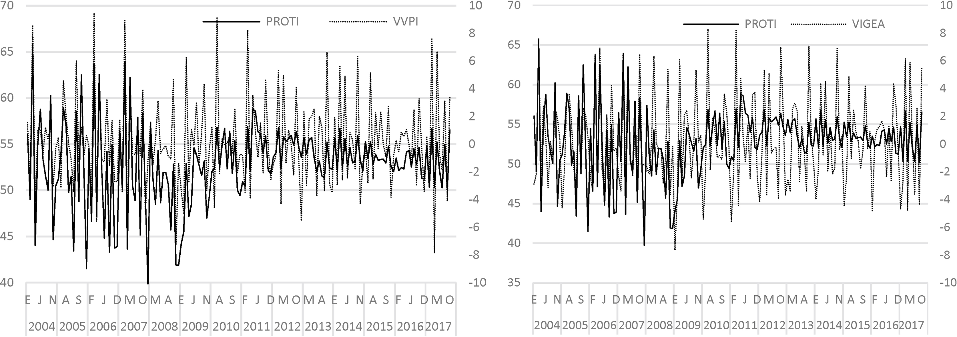
Due to the type of questions involved, ATI and MOI can only be compared with variables expressed as monthly differences or changes. For instance, Fig. 1 shows plots of ATI and the (quantitative) Volume of Production Index (VPI) expressed as monthly percent changes VVPI ${}_{t}=$ 100 $\times$ (VPI ${}_{t}$ /VPI ${}_{t-1}$ ) without and with seasonal adjustment. The two series follow similar direction patterns, but not necessarily of the same magnitude, so that their respective measurement scales should be indicated.

Table 1
Standard errors and critical values for cross-correlations with $N=$ 72

Lags	$\pm$ 6	$\pm$ 3	$\pm$ 2	$\pm$ 1	0
Standard error	0.123	0.120	0.120	0.119	0.118
Significance	Critical values
10%	$\pm$ 0.202	$\pm$ 0.198	$\pm$ 0.197	$\pm$ 0.195	$\pm$ 0.194
5%	$\pm$ 0.241	$\pm$ 0.236	$\pm$ 0.234	$\pm$ 0.233	$\pm$ 0.231
1%	$\pm$ 0.317	$\pm$ 0.310	$\pm$ 0.308	$\pm$ 0.306	$\pm$ 0.304

Table 2

Percentage of coincidences and cross-correlations between ATI and some quantitative variables

Coincidences	Cross-correlations: ATI ${}_{t+i}$ vs. VVPI ${}_{t}$
	i	$-$ 6	$-$ 3	$-$ 2	$-$ 1	0	1
83.1%	r(i)	$-$ 0.25 ${}^{**}$	$-$ 0.10	0.26 ${}^{**}$	$-$ 0.22 ${}^{*}$	0.59 ${}^{***}$	$-$ 0.14
	Cross-correlations: ATI ${}_{t+i}$ vs. VIGEA ${}_{t}$
77.5%	r(i)	$-$ 0.22 ${}^{*}$	$-$ 0.13	0.33 ${}^{***}$	$-$ 0.03	0.52 ${}^{**}$	$-$ 0.17
	Cross-correlations: ATI ${}_{t+i}$ vs. VVPI ${}_{t}$ deseasonalized
47.9%	r(i)	$-$ 0.03	$-$ 0.04	0.23 ${}^{*}$	$-$ 0.24 ${}^{**}$	0.31 ${}^{***}$	0.32 ${}^{***}$

Significance: ${}^{*}$ 10%, ${}^{**}$ 5% and ${}^{***}$ 1%.

Table 3

Percentage of coincidences and cross-correlations between the production and demand subindices of ATI with some quantitative variables

Coincidences	Cross-correlations: PROTI ${}_{t+i}$ vs. VVPI ${}_{t}$
	i	$-$ 6	$-$ 3	$-$ 2	$-$ 1	0	1
80.3%	r(i)	$-$ 0.28 ${}^{**}$	$-$ 0.09	0.23 ${}^{*}$	$-$ 0.27 ${}^{**}$	0.67 ${}^{***}$	$-$ 0.25 ${}^{**}$
	Cross-correlations: PROTI ${}_{t+i}$ vs. VIGEA ${}_{t}$
74.6%	r(i)	$-$ 0.21 ${}^{*}$	$-$ 0.14	0.30 ${}^{**}$	$-$ 0.07	0.59 ${}^{***}$	$-$ 0.29 ${}^{**}$
	Cross-correlations: DEMTI ${}_{t+i}$ vs. VIGEA ${}_{t}$
73.2%	r(i)	$-$ 0.26 ${}^{**}$	$-$ 0.15	0.32 ${}^{***}$	$-$ 0.15	0.56 ${}^{***}$	$-$ 0.25 ${}^{**}$

Significance: ${}^{*}$ 10%, ${}^{**}$ 5% and ${}^{***}$ 1%.

Figure 1.

Left panel: original series ATI (left scale) and VVPI (right scale). Right panel: seasonally adjusted series ATI and VVPI. January 2004–December 2009.

When two time series change from one month to the next one in the same direction we say that a coincidence occurred. The percentage of coincidences measures contemporary affinity between the two series, but no predictive ability can be claimed by getting a large percentage. It is the timeliness of the opinion indicators that makes them useful tools for the analysis of the current state of the economy. Another measure that quantifies association between two series is the cross-correlation coefficient for different lags and leads.

We do not attempt to establish any formal statistical comparison for the percentage of coincidences, nor indicate that a given percentage may be significantly different from zero, but just to observe if they are similar for different pairs of variables. On the contrary, the statistical significance of a cross-correlation can be established by referring it to a standard Normal distribution whose asymptotic variance is obtained as follows. If $r_{YX}(i)$ denotes an estimated cross-correlation between variables $Y$ and $X$ , with lags $i=$ 0, $\pm$ 1, $\pm$ 2, $\ldots$ , then its approximate variance (for large sample sizes, as in the present case) is given by

$\displaystyle\text{Var}[r_{YX}(i)]\approx 1/(N-i)$ (5)

where $N$ is the sample size. This approximation arises on the assumption that the two series under comparison are realizations of uncorrelated processes (see [7, Ch. 5]). To assign significance levels to a set of cross-correlations, we need to get the asymptotic standard errors of the coefficients and compare the signal to noise ratios (coefficient/standard error) with the critical values shown in Table 1. The value $N=$ 72 corresponds to the sample period January 2004–December 2009.

Table 2 presents the percentage of coincidences and some cross-correlation coefficients between ATI and some relevant quantitative variables, whose significance is indicated in order to decide if each of them (individually) can be considered different from zero. There we see that the contemporaneous correlations are the highest in the three cases and are significant at the 1% level. IGEA, expressed as a monthly variation is indicated with a V at the beginning of its name. The percentage of coincidences shown in Table 2 indicates that ATI has more affinity with VVPI than with VIGEA. Moreover, the contemporaneous correlation of ATI with VVPI is higher than that with VIGEA. Besides, the cross-correlations of order two point in the direction that ATI can be used to anticipate VIGEA and VVPI. Of course, this is just an exploratory analysis and we shall validate our findings in the next section.

In addition, we investigate the predictive ability of the subindices PROTI (production) on VVPI and VIGEA, and DEMTI (demand) on VIGEA. The plots of the series under comparison with PROTI appear in Fig. 2. The corresponding percentages of coincidences and cross-correlations appear in Table 3. It is clear that PROTI has lower percentages of coincidence but higher contemporaneous correlations with the respective quantitative variables than ATI. This apparently contradictory fact emphasizes the need of carrying out a confirmatory analysis. We see that cross-correlations in absolute value are higher for PROTI than for ATI and even the lead one cross-correlation is significant. Besides, we consider DEMTI because demand has a clear anticipatory content and the comparison is with VIGEA, the most relevant quantitative economic indicator. The results shown at the bottom of Table 3 are similar to those between PROTI and VIGEA.

Table 4

Percentage of coincidences and cross-correlations between MOI and some quantitative variables

Coincidences	Cross-correlations: MOI ${}_{t+i}$ vs. VVPI ${}_{t}$
	i	$-$ 6	$-$ 3	$-$ 2	$-$ 1	0	1
78.9%	r(i)	$-$ 0.21 ${}^{*}$	$-$ 0.07	0.15	$-$ 0.08	0.43 ${}^{***}$	$-$ 0.02
	Cross-correlations: MOI ${}_{t+i}$ vs. VIGEA ${}_{t}$
70.4%	r(i)	$-$ 0.20 ${}^{*}$	$-$ 0.06	0.21 ${}^{*}$	0.07	0.39 ${}^{***}$	$-$ 0.06
	Cross-correlations: MOI ${}_{t+i}$ vs. VVPI ${}_{t}$ deseasonalized
52.1%	r(i)	$-$ 0.06	0.05	0.15	0.27 ${}^{**}$	0.32 ${}^{***}$	0.34 ${}^{***}$

Significance: ${}^{*}$ 10%, ${}^{**}$ 5% and ${}^{***}$ 1%.

Figure 2.

Left panel: PROTI (left scale) and VVPI (right scale). Right panel: PROTI (left scale) and VIGEA (right scale).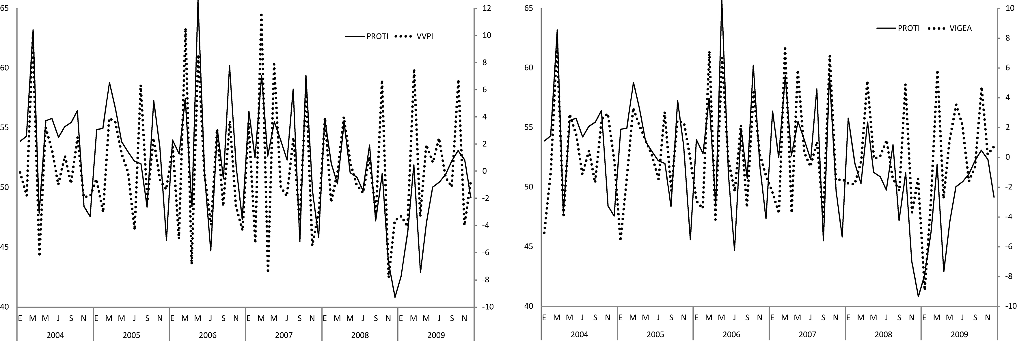

An aspect to be considered when analyzing time series is whether seasonal effects should be removed to obtain appropriate conclusions. For time series generated from opinion surveys, several studies have shown that they should be adjusted only when there is strong evidence of seasonality (e.g. [9] and the references therein). This recommendation arises because (i) there is no clear evidence of seasonality in opinion data and (ii) seasonal adjustment procedures are biased towards finding seasonality in series that do not have it. The OECD manual (see [13]) recommends analyzing each series individually to detect the ones that deserve being deseasonalized. We decided to compare the results previously obtained with those for the series adjusted for seasonality. To adjust the series we applied the Census Bureau X-12-ARIMA method (http://www.census.gov/srd/www/x12a/). As a result, we typically found a reduction in the affinity between the series, e.g. see Table 2 where the percentage of coincidences diminishes from 83.3% with the original series to 47.9% after adjusting it for seasonality. This happens because the quantitative variable gets modified substantially by the seasonal adjustment, as can be seen in Fig. 1. Furthermore, the seasonal adjustment produces some notorious changes in the cross-correlations, for instance, the correlation at lag 6 of ATI with VVPI was significant in the original series and became non-significant after deseasonalizing it. Something similar occurred with MOI when compared with VVPI, as shown in Table 4. Moreover, as shown in Section 5, the forecasting models derived in this work do not require seasonal coefficients. Thus, since our main objective is to get the most predictive information on quantitative variables from the survey data, we decided to work only with seasonally unadjusted series, [4] made the same decision.

Table 5

Percentage of coincidences and cross-correlations between expected and historical indices about production and demand

Coincidences	Cross-correlations: VPMOI ${}_{t+i}$ vs. PROTI ${}_{t}$
	i	$-$ 6	$-$ 3	$-$ 2	$-$ 1	0	1
83.1%	r(i)	$-$ 0.02	0.20 ${}^{*}$	0.39 ${}^{***}$	0.22 ${}^{*}$	0.82 ${}^{***}$	0.35 ${}^{***}$
	Cross-correlations: EDEMI ${}_{t+i}$ vs. DEMTI ${}_{t}$
71.8%	r(i)	0.06	0.36 ${}^{***}$	0.37 ${}^{***}$	0.46 ${}^{***}$	0.79 ${}^{***}$	0.46 ${}^{***}$

Significance: ${}^{*}$ 10%, ${}^{**}$ 5% and ${}^{***}$ 1%.

Figure 3.

Monthly mean values and standard deviations of approximate variations for Production, with and without trimming.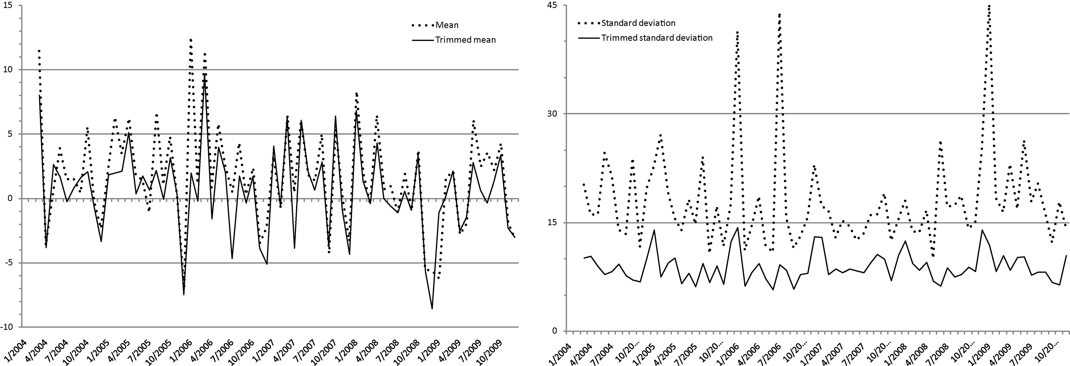

Another aspect worth of study is whether the data provided by the MBOS are internally coherent; for example, whether the subindex of expected production (VPMOI) anticipates the behavior of current production (PROTI). If so, we may say that the responses provide reliable information, otherwise the information may be suspect of lack of coherency. We should recall that this study involves diffusion indices (aggregated responses) and that fact did not allow us to study the internal coherency of the survey at the questionnaire level. Nevertheless, we found strong associations between expected and historical indicators for several variables considered by the MBOS. For example, Table 5 shows the percentage of coincidences and cross-correlations between expected and historical production and demand. Therefore, we may say that the historical opinion indices not only anticipate the economic fact, but are also contemporaneously correlated with expected opinion indicators, though the expected indicator is released one month before its historical counterpart. This result is important when trying to anticipate quantitative economic variables and gives support to the belief that the opinion indicators provide valid information to do that.

4. Further analysis of the MBOS

Aside from qualitative responses, the MBOS questionnaire asks the respondent for a numerical value that reflects his/her belief on the outcome of a variable by providing an Approximate Percent Variation, e.g. for Volume of production. These questions are usually considered sensitive, but according to the people in charge of the MBOS there is no particularly higher nonresponse for them. These questions can be asked because INEGI is an official statistical agency, so that the law enforces responding the questionnaire and protects confidentiality of the data. Perhaps a private organization would not get responses to these questions and that might be the reason for not including them in the questionnaire of that organization. It remains to show that the responses to such questions have predictive ability on economic facts.

We emphasize the questions referred to production and demand. The approximate variations are expressed as percentages and are related to the qualitative responses considered in Section 2, with positive content Much higher ( $j=$ 5) and Higher ( $j=$ 4) or with negative content Lower ( $j=$ 2) and Much lower ( $j=$ 1). The responses are summarized by the mean value of the approximate variations for variable X in month $t$ , calculated as follows

$\displaystyle\text{MVX}_{t}\!=\!\frac{\sum\limits_{i=1}^{n}(d_{5it}\!+\!d_{4it% }\!-\!d_{2it}\!-\!d_{1it})\text{AVX}_{i,t}p_{i}f_{i}}{\sum\limits_{i=1}^{n}p_{% i}f_{i}},$ (6)

Table 6

Descriptive statistics of the approximate variation series with and without trimming

Without trimming
Variable	Mean	Median	Standard dev	Mean dev	Skewness	Kurtosis
MVPRO	1.70	1.50	4.02	3.04	0.31	0.42
MVDEM	1.46	1.55	2.99	2.31	0.01	0.74
With trimming
MVPRO	0.55	0.64	3.45	2.60	$-$ 0.07	0.57
MVDEM	0.57	0.35	2.90	2.31	0.49	$-$ 0.06

Table 7

Percentage of coincidences and cross-correlations of MVPRO and MVDEM with some quantitative variables

Coincidences	Cross-correlations: MVPRO ${}_{t+i}$ vs. VVPI ${}_{t}$
	i	$-$ 6	$-$ 3	$-$ 2	$-$ 1	0	1
81.2%	r(i)	$-$ 0.27 ${}^{**}$	$-$ 0.20	0.37 ${}^{***}$	$-$ 0.40 ${}^{***}$	0.79 ${}^{***}$	$-$ 0.31 ${}^{**}$
	Cross-correlations: MVPRO ${}_{t+i}$ vs. VIGEA ${}_{t}$
76.8%	r(i)	$-$ 0.22 ${}^{*}$	$-$ 0.22 ${}^{*}$	0.45 ${}^{***}$	$-$ 0.13	0.60 ${}^{***}$	$-$ 0.38 ${}^{***}$
	Cross-correlations: MVDEM ${}_{t+i}$ vs. VIGEA ${}_{t}$
75.4%	r(i)	$-$ 0.25 ${}^{**}$	$-$ 0.09	0.30 ${}^{**}$	$-$ 0.26 ${}^{**}$	0.75 ${}^{***}$	$-$ 0.39 ${}^{***}$

Significance: ${}^{*}$ 10%, ${}^{**}$ 5% and ${}^{***}$ 1%.

Figure 4.

Left panel: MVPRO and VVPI series plotted in the same scale. Right panel: MVPRO and VIGEA series plotted in the same scale.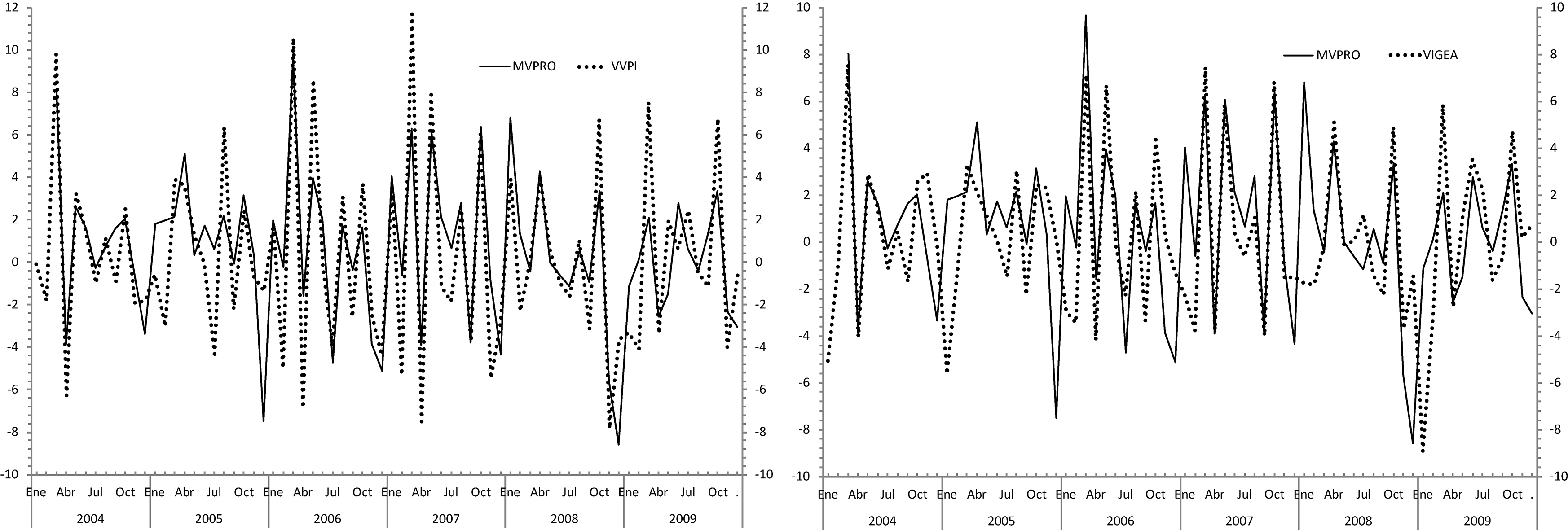

where $n$ is the number of firms in the sample, AVX ${}_{i,t}$ is the percent approximate variation of variable X reported by the i-th firm, $p_{i}$ is its weight (fixed asset), $f_{i}$ its expanding factor, and the dummy variable is such that $d_{jit}=$ 1 if the response of firm i is j and $d_{jit}=$ 0 otherwise.

At first sight, there is very large variability in the mean values and variances attributable to an exaggerate perception of the producers about growth (either positive or negative) in production and demand. In order to mitigate that effect we used trimmed means (we trimmed 5% at each end of the range, so that only the central 90% of the observations was employed). To appreciate the trimming effect on the production variable, in Fig. 3 (left panel) we show the series of mean values of the approximate variation for production with and without trimming. We can see that the level and dynamics of both series are similar, except for the extreme values. As a complement, the plots in the right panel show standard deviations, obtained as the square root of Eq. (7), for the original and trimmed approximate variations. The standard deviation for trimmed data is evidently lower than that of the original data, particularly for months with extreme observations.

Table 8

Estimation results of the forecasting models for VVPI. Estimation period: 2004:05*–2009:12

Model	VVPI lags	Predictors (with lags)	$\tilde{R}^{2}$ (%)	AIC	$\hat{\sigma}_{\varepsilon}$	Q* (24) p-value
AR	1, 4	–	40.5	5.25	3.274	0.11
ARX-1	1	ATI(0, 4)	67.5	4.66	2.421	0.75
ARX-2	1	PROTI(0, 4)	66.3	4.70	2.462	0.67
ARX-3	1-2, 4	VPMOI(0, 2-3, 5)	69.4	4.66	2.355	0.69
ARX-4	1-2, 5	MVPRO(0-2, 5)	81.6	4.18	1.850	0.85
ARX-5	1	ATI(4) & PROTI(0)	69.1	4.61	2.360	0.63
ARX-6	1, 5	ATI(4) & VPMOI(0, 5)	70.4	4.60	2.318	0.40
ARX-7	1, 5	ATI(4) & MVPRO(0-2, 5)	82.7	4.12	1.797	0.65
ARX-8	1, 5	PROTI(1, 3-4) & MVPRO(0, 2, 5)	82.8	4.13	1.794	0.63
ARX-9	1-2, 5	VPMOI(5) & MVPRO(0-2)	82.0	4.13	1.808	0.84

${}^{*}$ The estimation period starts in 2004:06 for models ARX(3, 6, 9) and in 2004:08 for ARX(4, 7, 8).

The trimming effect can also be seen in Table 6. Both the center of the data (measured as mean or median) and the dispersion (measured as standard deviation about the mean or as mean deviation around the median) get closer to zero for the trimmed data than for the original data, whereas the skewness and kurtosis coefficients fluctuate around zero and do not show a clear pattern. Thus, trimming does not alter the dynamics of the series and essentially reduces the variability associated to extreme values, thus allowing us to see the underlying signal more clearly. Hence, we decided to work with the series of trimmed means and from here on we refer only to this kind of data.

The exploratory analysis starts by looking at the coincidences and cross-correlations of the series under comparison. In Table 7 we present the results obtained for approximate variations against the quantitative series VVPI and VIGEA. This table is akin to Table 3, since the variables involved measure essentially the same thing. The same can be said about Fig. 4 as compared with Fig. 2. A comparison of the two tables indicates that the percentage of coincidences and the contemporaneous correlation increase for approximate variations. Not only affinity increased, but magnitudes become comparable, as can be seen in Fig. 4 where two pairs of series are plotted in the same scales.

5. A Forecasting experiment with opinion indices

Using opinion indices to improve prediction of a given variable is one of the main objectives to carry out opinion surveys. Several works (e.g. [1, 14]) have shown that such indices increase predictive ability of turning points. In order to check that such an objective is achieved by the MBOS we consider the information of the previous section to propose several forecasting models for VVPI and VIGEA.

We specified the forecasting models starting with an Auto-Regressive (AR) model for the quantitative variable of interest and incorporating opinion indices as exogenous variables. Such models will be referred to as ARX models. A typical ARX equation is

$\displaystyle Y_{t}=\alpha_{0}+\sum_{j=1}^{p}\alpha_{0,j}Y_{t-j}+\sum_{j=0}^{q% 1}\alpha_{1,j}X_{1,t-j}+\sum_{j=0}^{q2}\alpha_{2,j}X_{2,t-j}+\varepsilon_{t}$ (7)

Table 9

Estimation results of the forecasting models for VIGEA. Estimation period: 2004:05*–2009:12

Model	VIGEA lags	Predictors (with lags)	$\tilde{R}^{2}$ (%)	AIC	$\hat{\sigma}_{\varepsilon}$	Q* (24) Valor-p
AR	1, 12	–	36.5	4.91	2.745	0.73
ARX-1	1-2, 4	ATI(0, 2-3, 5)	49.6	4.65	2.344	0.09
ARX-2	2, 4	PROTI(0, 2- 3)	48.8	4.64	2.358	0.95
ARX-3	2, 12	DEMTI(0-4)	68.1	4.29	1.945	0.60
ARX-4	1-2, 4	VPMOI(0, 2-3, 5)	41.7	4.80	2.523	0.20
ARX-5	1-2	MVPRO(0, 2)	54.6	4.50	2.219	0.21
ARX-6	3-4	MVDEM(0)	58.2	4.41	2.131	0.30
ARX-7	2, 4-5	ATI(2) & DEMTI(0-1, 3)	64.6	4.30	1.965	0.65
ARX-8	2	DEMTI(0-1, 3-4) & PROTI(0-2)	62.6	4.36	2.015	0.46
ARX-9	2, 4-5	DEMTI(0-1, 3-4) & VPMOI(2, 4)	65.6	4.30	1.936	0.56
ARX-10	1-4	ATI(0, 5) & MVPRO(2, 4-5)	62.1	4.42	2.061	0.78
ARX-11	2, 4	PROTI(0,3, 5) & MVPRO(0, 2, 4-5)	62.3	4.42	2.056	0.46
ARX-12	1-2	DEMTI(0-1, 4) y MVPRO(1-2, 4)	69.9	4.17	1.824	0.43
ARX-13	1-2	VPMOI(5) & MVPRO(0, 2)	57.3	4.46	2.157	0.18
ARX-14	–	ATI(2, 4-5) & MVDEM(0)	61.9	4.33	2.038	0.09
ARX-15	4	PROTI(0, 2-3) & MVDEM(0)	61.4	4.36	2.048	0.26
ARX-16	12	DEMTI(2-4) & MVDEM(0)	73.1	4.09	1.785	0.86
ARX-17	3	VPMOI(2, 5) & MVDEM(0, 5)	60.0	4.43	2.117	0.49
ARX-18	–	MVPRO(2-3) & MVDEM(0, 4)	63.9	4.29	1.997	0.35

${}^{*}$ The estimation period starts in 2004:06 for models ARX(4, 7, 9, 13, 14), in 2004:07 for ARX(12, 18), in 2004:08 for ARX(10, 11) and in 2005:01 for AR and ARX(16).

where $Y$ is the quantitative variable to be forecasted and $X_{1}$ , $X_{2}$ are exogenous predictors (opinion indices or means of approximate variations). The parameters $\alpha_{0},\alpha_{0,1},\ldots,\alpha_{0,p}$ , $\alpha_{1,0},\ldots,\alpha_{1,q1}$ and $\alpha_{2,0},\ldots,\alpha_{2,q2}$ are estimated by OLS, so that { $\varepsilon_{t}$ } is assumed to be a zero-mean White Noise process with constant variance, $\sigma_{\varepsilon}^{2}$ . This variance is that of the one-period-ahead forecast we are interested in, so that the model can be used to produce interval, not just point forecasts. Moreover, the assumptions were validated with the data at hand as shown in the tables of the estimation results.

In all cases the AR model was augmented with one or at most two opinion indices or approximate variations previously found with predictive ability. A summary of the estimation and validation results of the models for VVPI is shown in Table 8, where the variables appear with their respective significant lags.

In Table 8 we also see the adjusted coefficient of determination $\tilde{R}^{2}$ , the Akaike Information Criterion AIC and the residual standard deviation, as well as the Ljung and Box (Q*) statistic with 24 degrees of freedom and its corresponding p-value, to judge model adequacy. The improvement in goodness of fit is sensibly larger when the opinion indices are included ( $\tilde{R}^{2}$ grows from 40.5% to 66.3% in the worst case and to 82.8% in the best one and AIC reduces from 5.25 to 4.12 in the best case). All ARX models include at least one predictor with significant lag 0 and there is no evidence of inadequacy in any model. In particular, we did not find any evidence of residual seasonality. Moreover, it should be noticed that the best predictor of VVPI is the mean of approximate variations of production, MVPRO, either considered alone or jointly with the tendency index of historical production, PROTI.

Similarly, in Table 9 we show the estimation results of the models for VIGEA. All models are valid in data according to the Ljung – Box statistic and DEMTI is the variable that considered alone best explains VIGEA ( $\tilde{R}^{2}=$ 68.1% and AIC $=$ 4.29). While the best pair of explanatory variables are DEMTI and MVDEM (73.1% and 4.09, respectively) so that demand provides the best explanation of VIGEA during the sample period. Again, let us notice that no residual seasonality appears and that some models include the 12-th lag of VIGEA.

To take advantage of the available data we must be aware of the releasing dates of the variables to be forecasted and their predictors. Figure 5 shows that the opinion indices on expectations OI(E) are released almost 40 days ahead of VPI and about 50 days ahead of IGEA. The anticipation of the opinion indices on historical performance OI(H) is smaller (about 10 and 22 days) but even so, its timing is relevant.

Figure 5.

Releasing dates of VVPI and VIGEA relative to the opinion indices provided by the MBOS, with reference to month t of a given quarter.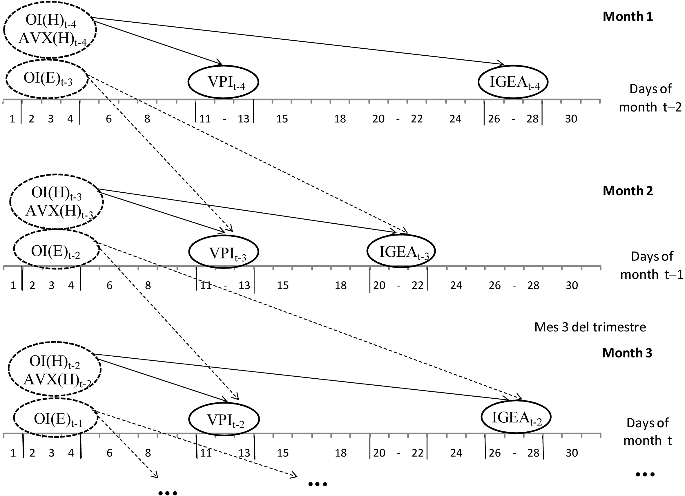

Table 10

Summary of the one-step-ahead forecasting results for VVPI

Model	ME	RMSE	Theil’s	Mincer-Zarnowitz equation
			U	$\hat{\eta}_{0}$	$t_{0}$	$\hat{\eta}_{1}$	$t_{1}$
AR	$-$ 0.57	3.40	1.00	$-$ 0.40	$-$ 0.43	$-$ 0.38	$-$ 1.06
ARX-1	$-$ 0.26	2.93	0.74	$-$ 0.24	$-$ 0.29	$-$ 0.14	$-$ 0.42
ARX-2	0.10	2.89	0.72	0.08	0.10	$-$ 0.09	$-$ 0.24
ARX-3	0.74	3.29	0.93	0.40	0.46	$-$ 0.38	$-$ 1.50
ARX-4	0.39	2.27	0.45	0.43	0.66	0.09	0.37
ARX-5	$-$ 0.43	2.60	0.58	$-$ 0.47	$-$ 0.64	0.16	0.47
ARX-6	$-$ 0.68	2.63	0.60	$-$ 0.61	$-$ 0.83	$-$ 0.12	$-$ 0.48
ARX-7	$-$ 0.47	2.09	0.38	$-$ 0.55	$-$ 0.96	0.21	0.93
ARX-8	$-$ 0.31	2.27	0.45	$-$ 0.33	$-$ 0.50	0.10	0.39
ARX-9	$-$ 0.61	2.05	0.36	$-$ 0.71	$-$ 1.29	0.22	1.00

Table 11

Summary of the one-step-ahead forecasting results for VIGEA

Model	ME	RMSE	Theil’s	Mincer-Zarnowitz equation
			U	$\hat{\eta}_{0}$	$t_{0}$	$\hat{\eta}_{1}$	$t_{1}$
AR	$-$ 0.09	3.69	1.00	$-$ 0.17	$-$ 0.15	$-$ 0.17	$-$ 0.32
ARX-3	0.32	3.25	0.78	0.42	0.42	0.12	0.27
ARX-4	0.51	4.26	1.33	$-$ 0.18	$-$ 0.14	$-$ 0.66	$-$ 1.36
ARX-5	0.26	3.27	0.79	0.65	0.65	0.49	0.89
ARX-6	$-$ 0.10	3.35	0.82	$-$ 0.02	$-$ 0.02	0.19	0.37
ARX-9	$-$ 0.26	3.91	1.12	$-$ 0.38	$-$ 0.35	$-$ 0.43	$-$ 0.98
ARX-12	$-$ 0.31	2.95	0.64	$-$ 0.33	$-$ 0.39	$-$ 0.08	$-$ 0.29
ARX-16	$-$ 0.32	3.19	0.75	$-$ 0.29	$-$ 0.31	0.13	0.32
ARX-18	0.14	3.20	0.75	0.19	0.20	0.08	0.19

The forecasting experiment is designed to compare the performance of one-step-ahead predictions for VVPI and VIGEA with the different ARX models in the post sample period 2009:01 to 2010:02 and each model in Table 8 produced monthly forecasts of VVPI for such a period. The models were reestimated each month, excluding the current and future values of VVPI and the one-step-ahead prediction was recorded. We calculated the one-step-ahead prediction errors for the 14 post sample values and Table 10 presents the following summary measures: (i) Mean Error (ME) to check for potential prediction biases, (ii) Root Mean Square Error (RMSE) as a measure of precision expressed in the same units of the variable and (iii) Theil’s U statistic as a measure of relative precision against that of a benchmark model (the AR model in this case). The interested reader is referred to [6] for details on these measures. We do not present the Mean Absolute Error because it provides basically the same information as the RMSE (see [8]).

Further empirical support to the forecasting models is provided by the Mincer-Zarnowitz equation (see [6, Ch. 11]) which is useful to verify that all the information available was efficiently employed by the model in turn, that is,

$\displaystyle e_{t}=\eta_{0}+\eta_{1}\hat{Z}_{t-1}(1)+u_{t},$ (8)

where { $u_{t}$ } is a sequence of uncorrelated zero-mean random errors with constant variance. In this sense, the forecast is optimal when $\eta_{0}=\eta_{1}=$ 0. The estimated coefficients and their $t$ -statistics are shown in Table 10 for each model under consideration.

In Table 10 we can see that none of the models shows significant non-zero bias. This fact indicates that the models make efficient use of their corresponding information sets. Moreover, the Theil’s U statistics show that the inclusion of an exogenous variable to the AR model increases predictive ability over VVPI. By looking at the RMSEs and Theil’s U statistics it is clear that the best model is the ARX-9 that incorporates MVPRO as predictor. It should be stressed that this model was among those with best goodness of fit.

The explicit expression of the recommended ARX-9 model to get one-step-ahead predictions of VVPI is

$\displaystyle\text{V$\hat{\text{V}}$PI}_{t-1}(1)=\hat{\alpha}_{0}+\hat{\alpha}% _{0,1}\text{VVPI}_{t-1}+\hat{\alpha}_{0,2}\text{VVPI}_{t-2}+\hat{\alpha}_{0,5}% \text{VVPI}_{t-5}+\hat{\alpha}_{1,5}\text{VPMOI}_{t-5}+\hat{\alpha}_{2,0}\text% {MVPRO}_{t}+\hat{\alpha}_{2,1}\text{MVPRO}_{t-1}+\hat{\alpha}_{2,2}\text{MVPRO% }_{t-2}$ (9)

where $\hat{\alpha}_{0}=$ 10.45 (3.44), $\hat{\alpha}_{0,1}=$ $-$ 0.54 ( $-$ 4.63), $\hat{\alpha}_{0,2}=$ $-$ 0.26 ( $-$ 2.21), $\hat{\alpha}_{0,5}=$ 0.15 (2.25), $\hat{\alpha}_{1,5}=$ $-$ 0.21 ( $-$ 3.59), $\hat{\alpha}_{2,0}=$ 0.77 (10.05), $\hat{\alpha}_{2,1}=$ 0.21 (1.81) and $\hat{\alpha}_{2,2}=$ 0.46 (3.97), with t-statistics in parenthesis and $\hat{\sigma}_{\varepsilon}=$ 1.808, $\tilde{R}^{2}=$ 0.82. Thus, a point forecast of the index VPI is obtained from

$\displaystyle\text{V$\hat{\text{P}}$I}_{t-1}(1)=\text{V $\hat{\text{V}}$PI}_{t% -1}(1)\times\text{VPI}_{t-1}/100$ (10)

and a 95% prediction interval is given by

$\displaystyle\text{[V$\hat{\text{V}}$PI}_{t-1}(1)\pm 1.96\hat{\sigma}_{% \varepsilon}]\times\text{VPI}_{t-1}/100.$ (11)

Table 11 shows a summary of the prediction errors for several models employed to forecast VIGEA. We present only the results for models with higher forecast precision and higher $\tilde{R}^{2}$ values. None of these models have a significant non-zero bias according to the Mincer-Zarnowitz estimated equation.

With regard to precision, Table 11 allows us to see that the best model is the ARX-12 (that includes DEMTI and MVPRO) which also has one of the highest $\tilde{R}^{2}$ values of all the entertained models. Its explicit expression becomes

$\displaystyle\text{VI$\hat{\text{G}}$EA}_{t-1}(1)=\hat{\alpha}_{0}+\hat{\alpha% }_{0,1}\text{VIGEA}_{t-1}$ $\displaystyle\quad+\hat{\alpha}_{0,2}\text{VIGEA}_{t-2}+\hat{\alpha}_{1,0}% \text{DEMTI}_{t}$ $\displaystyle\quad+\hat{\alpha}_{1,1}\text{DEMTI}_{t-1}+\hat{\alpha}_{1,4}% \text{DEMTI}_{t-4}$ $\displaystyle\quad+\hat{\alpha}_{2,1}\text{MVPRO}_{t-1}+\hat{\alpha}_{2,2}% \text{MVPRO}_{t-2}$ $\displaystyle\quad+\hat{\alpha}_{2,4}\text{MVPRO}_{t-4}$ (12)

where $\hat{\alpha}_{0}=$ 3.31 (0.85), $\hat{\alpha}_{0,1}=$ $-$ 0.25 ( $-$ 2.23), $\hat{\alpha}_{0,2}=$ $-$ 0.28 ( $-$ 2.53), $\hat{\alpha}_{1,0}=$ 0.36 (6.60), $\hat{\alpha}_{1,1}=$ $-$ 0.15 ( $-$ 1.91), $\hat{\alpha}_{1,4}=$ $-$ 0.28 ( $-$ 4.04), $\hat{\alpha}_{2,1}=$ 0.32 (3.12), $\hat{\alpha}_{2,2}=$ 0.54 (5.63) and $\hat{\alpha}_{2,4}=$ 0.22 (2.09), with $\hat{\sigma}_{\varepsilon}=$ 1.824 and $\tilde{R}^{2}=$ 0.699. Point and interval predictions for IGEA can be obtained again with formulas similar to Eqs (10) and (11).

6. Conclusions

The coincidence and cross-correlation analyses are very simple and easy-to-use exploratory tools that helped us to select a few opinion indicators from a large list of potential predictors for relevant macroeconomic variables. An opinion indicator may be considered a good predictor because it indeed shows anticipatory power on the quantitative variable of interest. However, it suffices that both the indicator and the variable move contemporaneously to select the respective indicator as a useful predictor, due to its timely publication. Thus, we suggest applying this type of analysis routinely with the opinion indices generated from opinion surveys.

With respect to the forecasting models, this work lends support to the use of opinion indices from the MBOS to improve the prediction of VVPI and VIGEA, since these variables can be best predicted when the contemporaneous values of MVPRO and DEMTI are used, correspondingly. We should stress that MVPRO is an opinion variable that had never been used before in Mexico to improve the predictive ability on important macroeconomic variables. We strongly recommend the use of this kind of variables, whenever the corresponding question can be asked in the questionnaire of an opinion survey, because the data generated this way was seen here to have high predictive power on the corresponding quantitative variable (to signal both direction and size of change).

The main conclusion is that opinion indices are useful to generate timely nowcasts and improve the forecasting ability of time series models for some important Mexican macroeconomic variables.

Footnotes

Acknowledgments

This work was carried out in collaboration with the INEGI personnel. Víctor M. Guerrero acknowledges financial support from Asociación Mexicana de Cultura, A. C. to carry out this work.

A Partial Update with Some Data up to October 2017

The basic aim of this section is to show that the original patterns seen in the graphs obtained in the previous version of this paper remain valid, even though the variability of the ATI indicator diminishes notably due to the increase of sample size starting in 2011. In fact, we can summarize the new results by saying that the previously observed (graphical and numerical) patterns remain valid, and they even become more statistically significant than before.

Table A.1

Standard errors and critical values for cross-correlations with N $=$ 166

Lags	$\pm$ 6	$\pm$ 3	$\pm$ 2	$\pm$ 1	0
Standard error	0.079	0.078	0.078	0.078	0.078
Significance	Critical values
10%	$\pm$ 0.130	$\pm$ 0.129	$\pm$ 0.128	$\pm$ 0.128	$\pm$ 0.128
5%	$\pm$ 0.155	$\pm$ 0.154	$\pm$ 0.153	$\pm$ 0.153	$\pm$ 0.152
1%	$\pm$ 0.204	$\pm$ 0.202	$\pm$ 0.201	$\pm$ 0.201	$\pm$ 0.200

Table A.2

Percentage of coincidences and cross-correlations between ATI and some quantitative variables

Coincidences	Cross-correlations: ATI ${}_{t+i}$ vs. VVPI ${}_{t}$
	i	$-$ 6	$-$ 3	$-$ 2	$-$ 1	0	1
81.2%	r(i)	$-$ 0.23 ${}^{***}$	$-$ 0.08	0.22 ${}^{***}$	$-$ 0.29 ${}^{***}$	0.59 ${}^{***}$	$-$ 0.20 ${}^{**}$
	Cross-correlations: ATI ${}_{t+i}$ vs. VIGEA ${}_{t}$
79.4%	r(i)	$-$ 0.17 ${}^{**}$	$-$ 0.17 ${}^{**}$	0.27 ${}^{***}$	$-$ 0.13 ${}^{*}$	0.52 ${}^{***}$	$-$ 0.20 ${}^{**}$
	Cross-correlations: ATI ${}_{t+i}$ vs. VVPI ${}_{t}$ deseasonalized
46.7%	r(i)	$-$ 0.10	0.04	0.20 ${}^{**}$	0.25 ${}^{***}$	0.21 ${}^{***}$	0.22 ${}^{***}$

Significance: ${}^{*}$ 10%, ${}^{**}$ 5% and ${}^{***}$ 1%.

Figure A.1.

Left panel: original series ATI (left scale) and VVPI (right scale). Right panel: seasonally adjusted series ATI and VVPI. January 2004–October 2017.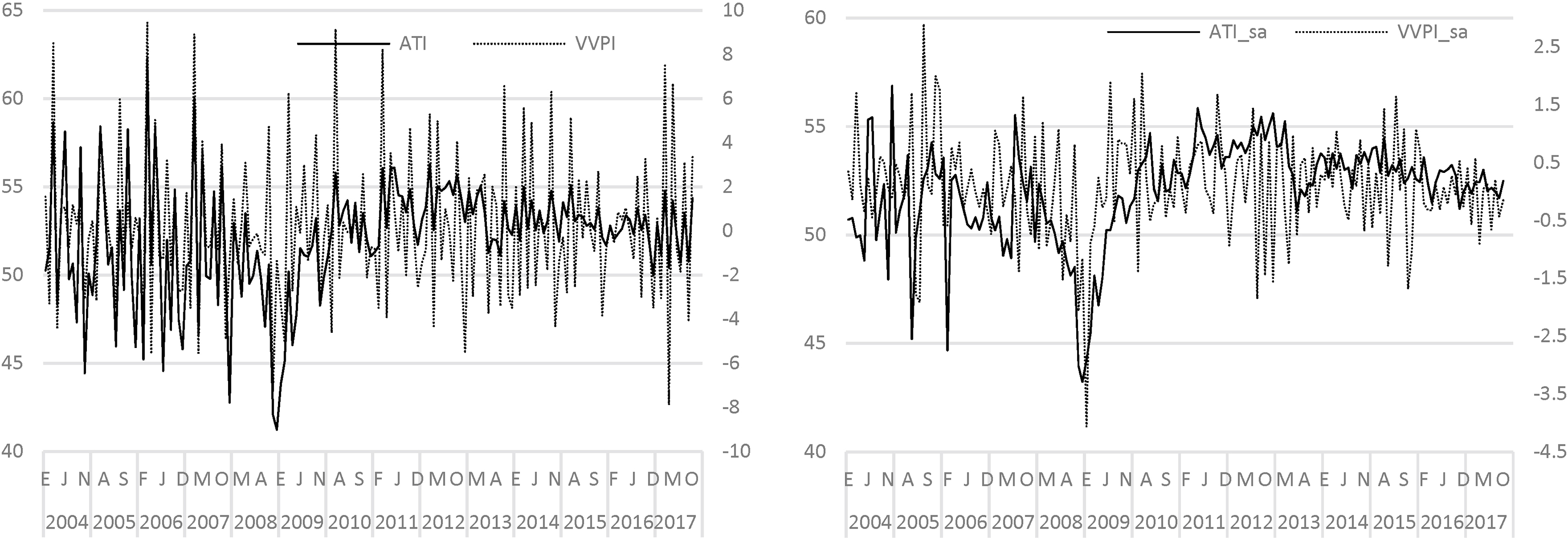

Table A.3

Percentage of coincidences and cross-correlations between the production and demand subindices of ATI with some quantitative variables

Coincidences	Cross-correlations: PROTI ${}_{t+i}$ vs. VVPI ${}_{t}$
	i	$-$ 6	$-$ 3	$-$ 2	$-$ 1	0	1
84.2%	r(i)	$-$ 0.29 ${}^{***}$	$-$ 0.11	0.29 ${}^{***}$	$-$ 0.36 ${}^{***}$	0.65 ${}^{***}$	$-$ 0.30 ${}^{***}$
	Cross-correlations: PROTI ${}_{t+i}$ vs. VIGEA ${}_{t}$
76.4%	r(i)	$-$ 0.25 ${}^{***}$	$-$ 0.15 ${}^{*}$	0.34 ${}^{***}$	$-$ 0.22 ${}^{***}$	0.53 ${}^{***}$	$-$ 0.28 ${}^{***}$
	Cross-correlations: DEMTI ${}_{t+i}$ vs. VIGEA ${}_{t}$
79.4%	r(i)	$-$ 0.14 ${}^{*}$	$-$ 0.14 ${}^{*}$	0.18 ${}^{**}$	$-$ 0.17 ${}^{**}$	0.60 ${}^{***}$	$-$ 0.24 ${}^{***}$

Significance: ${}^{*}$ 10%, ${}^{**}$ 5% and ${}^{***}$ 1%.

Table A.4

Percentage of coincidences and cross-correlations between MOI and some quantitative variables

Coincidences	Cross-correlations: MOI ${}_{t+i}$ vs. VVPI ${}_{t}$
	i	$-$ 6	$-$ 3	$-$ 2	$-$ 1	0	1
80.6%	r(i)	$-$ 0.24 ${}^{***}$	$-$ 0.11	0.18 ${}^{**}$	$-$ 0.21 ${}^{***}$	0.51 ${}^{***}$	$-$ 0.16 ${}^{**}$
	Cross-correlations: MOI ${}_{t+i}$ vs. VIGEA ${}_{t}$
76.4%	r(i)	$-$ 0.15 ${}^{*}$	$-$ 0.15 ${}^{*}$	0.22 ${}^{***}$	$-$ 0.08	0.46 ${}^{***}$	$-$ 0.16 ${}^{**}$
	Cross-correlations: MOI ${}_{t+i}$ vs. VVPI ${}_{t}$ deseasonalized
56.4%	r(i)	$-$ 0.07	$-$ 0.01	0.20 ${}^{**}$	0.24 ${}^{***}$	0.23 ${}^{***}$	0.20 ${}^{**}$

Significance: ${}^{*}$ 10%, ${}^{**}$ 5% and ${}^{***}$ 1%.

Table A.5

Percentage of coincidences and cross-correlations between expected and historical indices about production

Coincidences	Cross-correlations: VPMOI ${}_{t+i}$ vs. PROTI ${}_{t}$
	i	$-$ 6	$-$ 3	$-$ 2	$-$ 1	0	1
83.0%	r(i)	$-$ 0.19 ${}^{**}$	0.03	0.31 ${}^{***}$	$-$ 0.09	0.85 ${}^{***}$	$-$ 0.04

Significance: ${}^{*}$ 10%, ${}^{**}$ 5% and ${}^{***}$ 1%.

Figure A.2.

Left panel: PROTI (left scale) and VVPI (right scale). Right panel: PROTI (left scale) and VIGEA (right scale).

References

Abberger

. Qualitative business surveys and the assessment of employment – A case study for Germany. International Journal of Forecasting. 2007; 23: 249-258.

Batchelor

, and Dua

. Improving macro-economic forecasts. The role of consumer confidence. International Journal of Forecasting. 1998; 14: 71-81.

Cabrera

, and Salazar

. Las Encuestas de Opinión en el Análisis del Ciclo Económico Salvadoreño: Un análisis exploratorio. Tópicos Económicos. April 2009; 2(31): 1-18. Central Reserve Bank of El Salvador.

Claveria

Pons

, and Ramos

. Business and consumer expectations and macroeconomic forecasts. International Journal of Forecasting. 2007; 23: 47-69.

ECB. Opinion Surveys on Activity, Prices and Labour Market Developments in the Euro Area: Features and Uses. Monthly Bulletin. January 2004: 51–61. European Central Bank.

Diebold

. Elements of Forecasting. 2nd edition. 2001; South-Western, Cincinnati.

Enders

. Applied Econometric Time Series. Second edition. 2004; John Wiley and Sons, Inc. USA.

Granger

CWJ

. Can We Improve the Perceived Quality of Economic Forecasts? Journal of Applied Econometrics. 1996; 11: 455-473.

Guidetti

Gyomai

, and Spinelli

. Is it necessary to seasonally adjust business and consumer confidence series? Presented at the Fourth Joint EU-OECD Workshop on Business and Consumer Opinion Surveys. Brussels, 12–13 October 2009.

10.

Hansson

Jansson

, and Löf

. Business survey data: Do they help in forecasting GDP growth? International Journal of Forecasting. 2005; 21: 377-389.

11.

INEGI. Ley del Sistema Nacional de Información Estadística y Geográfica. 2nd edition. 2008; México, Aguascalientes.

12.

INEGI. Encuesta Mensual de Opinión Empresarial. Síntesis metodológica. Indicadores de opinión del sector manufacturero (EMOE). Instituto Nacional de Estadística y Geografía. 2009; México, Aguascalientes.

13.

OECD. Business Tendency Surveys: A Handbook. OECD: Paris, France. 2003; Available at http://www.oecd.org/dataoecd/37/42/42495745.pdf.

14.

Öller

. Forecasting the business cycle using survey data. International Journal of Forecasting. 1990; 6: 453-461.

15.

Rahiala

, and Teräsvirta

. Business survey data in forecasting the output of Swedish and Finnish metal and engineering industries: A Kalman filter approach. Journal of Forecasting. 1993; 12: 255-271.

An updated analysis of the predictive ability of Mexico’s Manufacturing Business Opinion Survey 1

Abstract

Keywords

1. Introduction

2. Monthly manufacturing business opinion survey

Table 1 Standard errors and critical values for cross-correlations with N = 72

Footnotes

Acknowledgments

A Partial Update with Some Data up to October 2017

References

Table 1
Standard errors and critical values for cross-correlations with $N=$ 72