






Abstract
Poverty indicators purely based on income statistics do not reflect the full picture of household’s economic well-being. Consumption and wealth are two additional key dimensions that determine the economic opportunities of people or material inequalities. We use non-parametric statistical matching methods to join consumption data from the Household Budget Survey to micro data from the European Union Statistics on Income and Living Conditions. In a second step, micro data from the Household Finance and Consumption Survey are joint to produce a common distribution of income, consumption and wealth variables. A variety of different indicators is then produced based on this joint data set, in particular household saving rates. Care has to be taken when interpreting the indicators, since the statistical matching is based on strong assumptions and a limited number of variables common to all of the three original data sets. We are able to show, however, that the assumptions made are justified by the use of strong proxies as matching variables. Thus, the resulting indicators have the potential to contribute to the analysis of inequality patterns and enhance the possibilities of social, and possibly fiscal, policy impact analysis.
Introduction
Building a fairer Europe and strengthening its social dimension is a key priority on the political agenda of the European Commission. Monitoring this goal requires suitable indicators bringing the social dimension on a par with macroeconomic measures. The best indicators currently available to monitor distributional aspects and inequality in the society are the ones based on the European Union Statistics on Income and Living Conditions (EU-SILC). The EU-SILC is a survey collecting annual microdata on income, poverty, social exclusion and living conditions in all EU member states. Multiple statistics are produced from these data, most prominently the at-risk-of-poverty (AROP) indicator, also combined with information on work intensity and material deprivation (AROPE). Due to the main focus of the survey, all indicators based on EU-SILC are income driven.
We argue that for getting the full picture of household’s economic situation, income based indicators should be enhanced by consumption behaviours and the ability of households to set aside part of their income as savings. Consumption behaviours best reflect the necessity of households whereas savings permit to level out irregularities in the usual income or necessity. A further component of economic well-being is the household’s accumulated wealth, since wealth has an impact on the household’s capacity to continue consuming in the event of a sudden loss of income.
Harmonised EU statistics covering the distributional aspects of households’ income, consumption and wealth (ICW) in a joint data set could thus help to reach the goals of the European Union’s economic governance framework by monitoring socio-economic trends in EU countries. They could further contribute to the impact analysis of fiscal policies.
In this paper, we use statistical matching methods to join income, consumption and wealth variables from different household surveys into a single micro data set for EU countries. We use income data from the European Union Statistics on Income and Living Conditions (EU-SILC), consumption data from the European Household Budget Survey (HBS) and wealth data from the Eurosystem Household Finance and Consumption Survey (HFCS).1 We outline the methodology used and the quality of the matching achieved, then present some indicators that can be compiled from the joint micro data set. In particular, the joint SILC-HBS micro data set permits us to calculate savings as the difference of income and expenditure. This exercise has first been conducted for the reference year 2010 and now been repeated for 2015 data. We can thus compare the results for these two years.2
Methodology
Background
The best data set including income, consumption and wealth variables would most likely be obtained through an integrated survey collecting data on the three dimensions from the same households at the same time. This approach is hardly used though due to the excessive response burden, and thus high non-response rates, of such a survey. In addition, allocating weights suitable for all of the three dimensions is rather difficult. In Europe, Hungary (since 2012) and Czechia (since 2017) [1] are the only countries to collect income (EU-SILC) and expenditure (HBS) data through one single survey. Czechia even plans to integrate wealth data by 2020.
Potential matching variables available in both EU-SILC and HBS. (“derived” indicates that the variable has been computed based on other variables in the data set)
Potential matching variables available in both EU-SILC and HBS. (“derived” indicates that the variable has been computed based on other variables in the data set)
Another option for obtaining joint income, consumption and wealth data sets is linking records with unique identifiers from several data sources, if these data are suitable for the measurement of the sought dimensions. This method is mostly in use in countries with administrative registers providing the desired information, essentially on income and wealth. In Europe, these are typically the Northern countries with Finland being the most prominent case linking wealth variables from the HFCS with EU-SILC [2, 3], although more and more countries are now using fiscal data to measure income.
Most EU countries, however, do not collect data on the three economic dimensions in an integrated survey and do not have the possibility to link records from different data sources either. This is why none of the above methods is applicable in a centralized exercise for all EU countries. For producing an income-consumption or income-consumption-wealth data set using the same methodology for all countries we need to resort to statistical methods which allow to combine the respective EU-wide surveys based on common information. A variety of such statistical matching methods exists and is thoroughly described in [4]. Several (unpublished) experiments were conducted on EU-SILC and HBS data for some of these methods (random hot-deck, rank hot-deck, distance hot-deck, mixed approach) focusing on countries with a high conceptual correspondence between disposable income in EU-SILC and income in HBS.3 Non-parametric methods were preferred over parametric ones as they are generally assumption-free regarding the parameters of the distributions. Likewise, methods such as distance hot-deck, more suitable for a statistical matching with a large number of matching variables, turned out to be unnecessary for this experiment. Instead, the non-parametric random hot-deck method was retained as well suited for the statistical matching of SILC and HBS data because it performed best in preserving the original distributions of income and consumption observed in the original EU-SILC and HBS data in the matched data set. Likewise, the rank hot-deck method was chosen for the matching of SILC and HFCS data. These two exercises are thus explained in the following sections. It should be kept in mind though that both of these methods rely on the conditional independence assumption, which can hardly be verified.
Statistical matching generally implies joining two different data sets
Variable selection
Our variables of interest
Comparability between the matching variables of the two data sets is essential and has been assessed using the Hellinger distance. As a rule of thumb, a Hellinger distance of below 0.05 indicates variables that are regarded as sufficiently comparable to be used for the matching. Applied to categorical variables
In addition, the Chi-2 test has been used to test the similarity of the distributions and account for sampling variances.
Finally, it is important to note that the EU-SILC, HBS and HFCS surveys have a different periodicity and variations of the reference year may occur for different countries even within the same survey waves. For each country, we use EU-SILC data corresponding to the same reference year around 2010 and 2015 available in HBS, and choose HFCS data with the closest reference year available to that (Table 2).
Reference years “around 2010” and “around 2015” in EU-SILC, HBS and HFCS
Once the potential matching variables have been selected, we identify the best subset for stratifying the households in the EU-SILC and HBS data sets. This has to be seen as a trade-off between the predictive power of the target variables and making the conditional independence assumption more plausible on the one hand, and the number of candidate households in each stratum on the other hand to avoid that there might be insufficient households to perform the matching. The following algorithm ensures a reasonable minimal size of strata while selecting the most relevant matching variables:
Step 1, a step-by-step linear backward selection regression model to select at most the Step 2, the stratification of both data sets according to the variables
where Step 3, if this threshold does not hold, the process is reiterated with the selection of
This approach results in the selection of different sets of actual matching variables for the countries depending on the predictive power of each of the potential variables in the country and on the sample sizes. However, the methodology used remains the same for all of the countries; hence it can be considered as a harmonised approach for all countries. Moreover, the income variable divided in 20 quantiles and highly correlated with the target variables has been selected as a matching variable for all the countries. The fact that the list of matching variables includes a proxy of one of the target variables makes the CIA a more justifiable and plausible assumption [6].
Probability density function of total consumption from original HBS data and the matched data set for Austria. The shaded area reflects the 95% confidence interval obtained from the 100 repetitions of the matching process.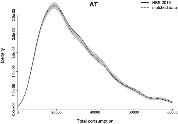
After the successful stratification of EU-SILC and HBS data, each EU-SILC household receives the consumption value from a random HBS household from within the same stratum, meaning with similar household characteristics. In addition, following Renssen [7], we re-calibrate the set of weights from EU-SILC to account both for EU-SILC and HBS margins. The whole process is replicated 100 times to assess the uncertainty related to this matching procedure in form of a between-imputation variance or a confidence interval. For the estimates presented in the results section, the weighted mean of the 100 iterations is used.
For joining wealth data to the income/consumption data set we make use of the gross income variable which is available both in HFCS and in EU-SILC. This variable is sufficiently comparable between both data sets to be used for a ranking of households and, due to its high correlation, it can be considered as a proxy variable of total disposal income. In this way, the CIA between total disposal income and total assets given the proxy can be justified. Again, we harmonise first the common variables available in both data sets, then we stratify our SILC-HBS and HFCS data sets according to a set of common variables that account for consumption and wealth: the household type, the tenure status and the food consumption quintile. This last variable is highly correlated with the total consumption expenditures and can thus be considered a good proxy, justifying the CIA between total consumption expenditure and total assets.
The process is replicated 100 times to provide a confidence interval for the matching, and the weighted mean of the 100 iterations is used for estimating the results. The final output of the matching exercise is a synthetic data set composed of the target variables of the three sources and the matching variables used, limiting the secondary analysis to that concrete set.
Quality of the matching
We assess the quality of the statistical matching by comparing the original distribution of total consumption in the HBS data set with total consumption in the matched SILC-HBS data set. Figures 1–3 show examples of this comparison for three exemplary countries, Austria, Greece and Latvia for 2015 data. The probability density functions show good results of the income-consumption matching. As for these three countries, this is mostly the case for the other EU27 countries too and it is confirmed by Table 3, which shows the gap between the cumulative distribution of consumption in the matched data set as compared to the original data.
Summary table of the gap (%) in the distribution of original HBS consumption and consumption in the matched data set (2015)
Summary table of the gap (%) in the distribution of original HBS consumption and consumption in the matched data set (2015)
Probability density function of total consumption from original HBS data and the matched data set for Greece. The shaded area reflects the 95% confidence interval obtained from the 100 repetitions of the matching process. 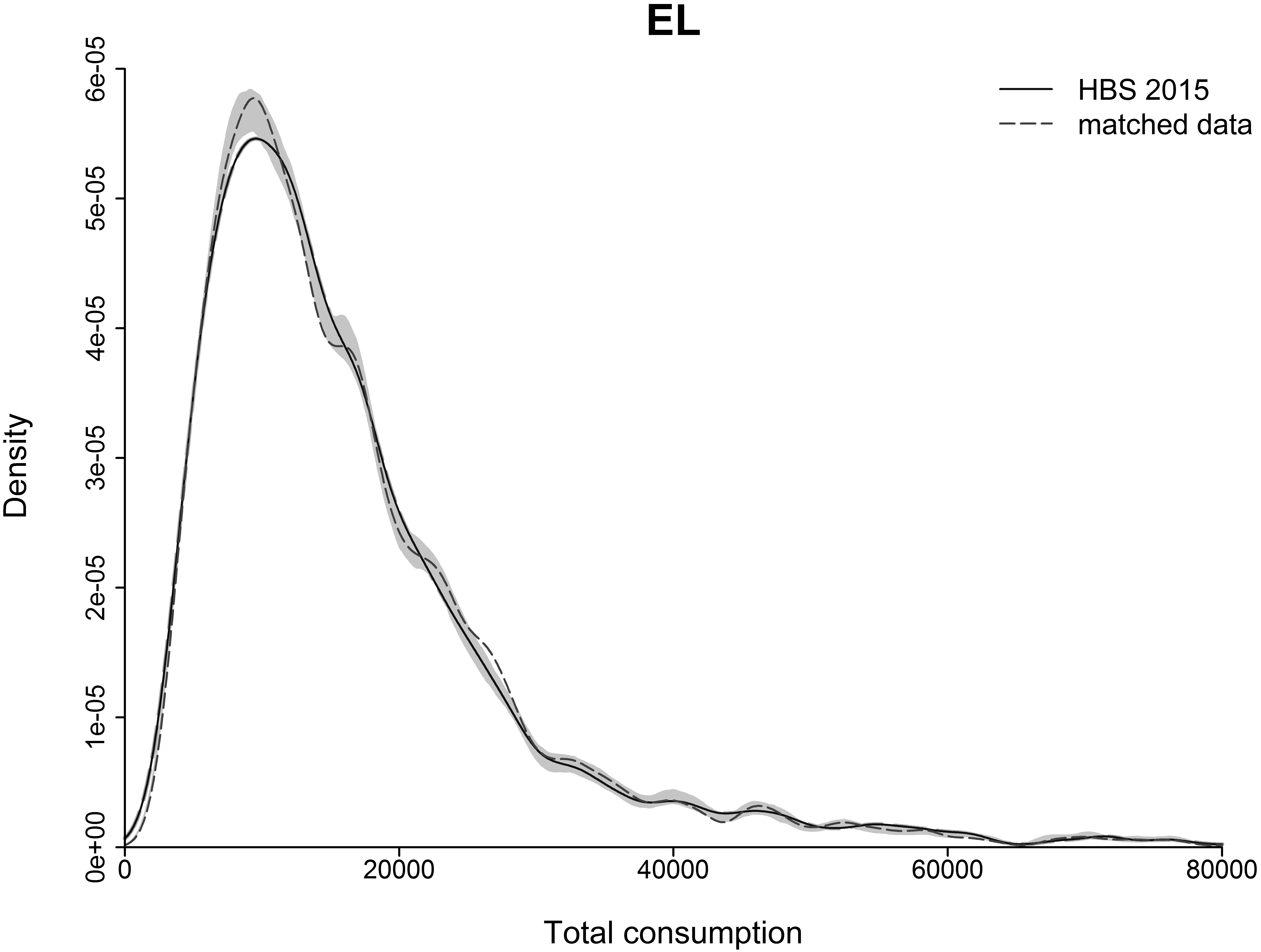
Probability density function of total consumption from original HBS data and the matched data set for Latvia. The shaded area reflects the 95% confidence interval obtained from the 100 repetitions of the matching process.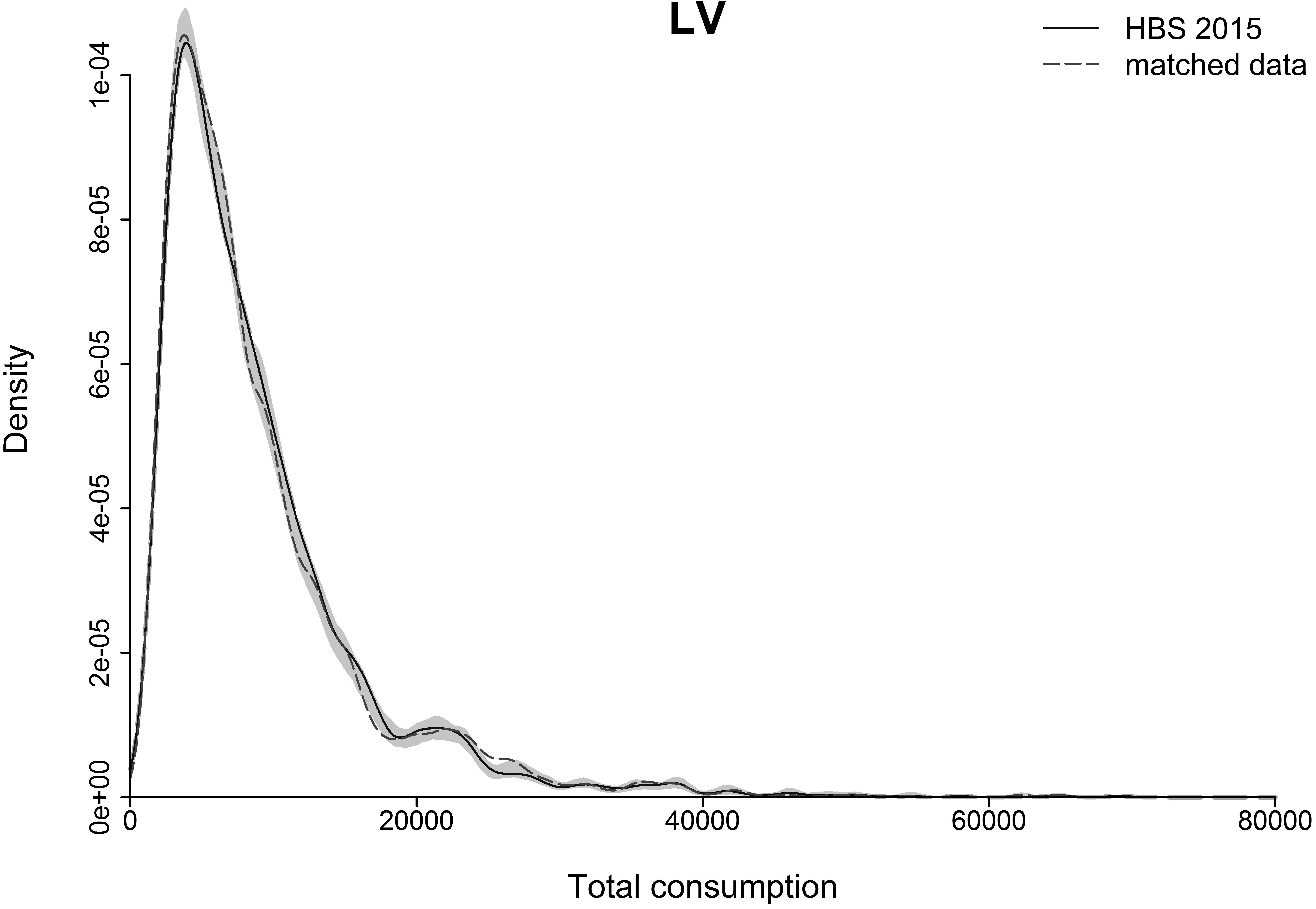
Probability density function of total assets from original HFCS data and the matched data set for Austria. The shaded area reflects the 95% confidence interval obtained from the 100 repetitions of the matching process. 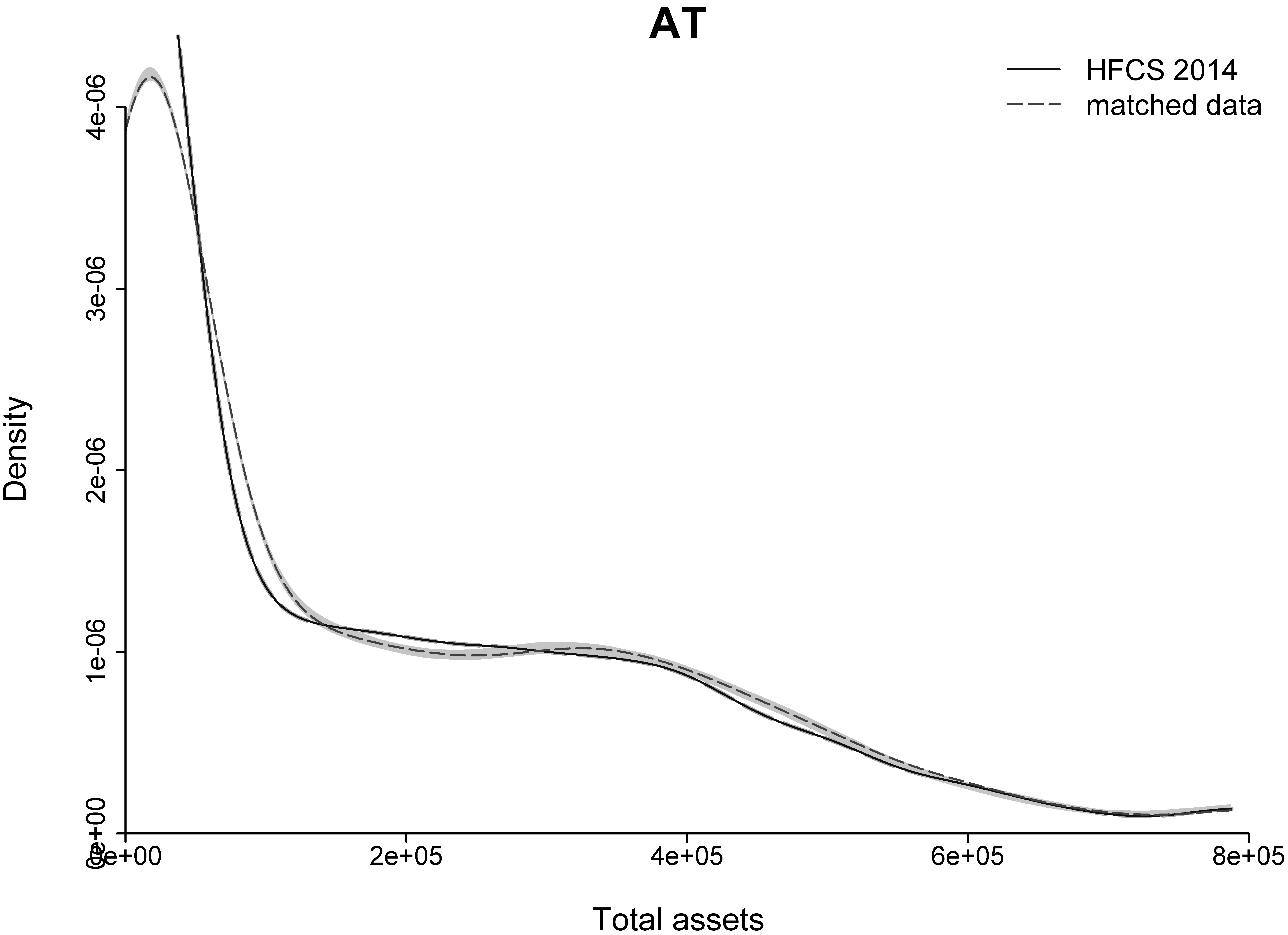
Probability density function of total assets from original HFCS data and the matched data set for Greece. The shaded area reflects the 95% confidence interval obtained from the 100 repetitions of the matching process. 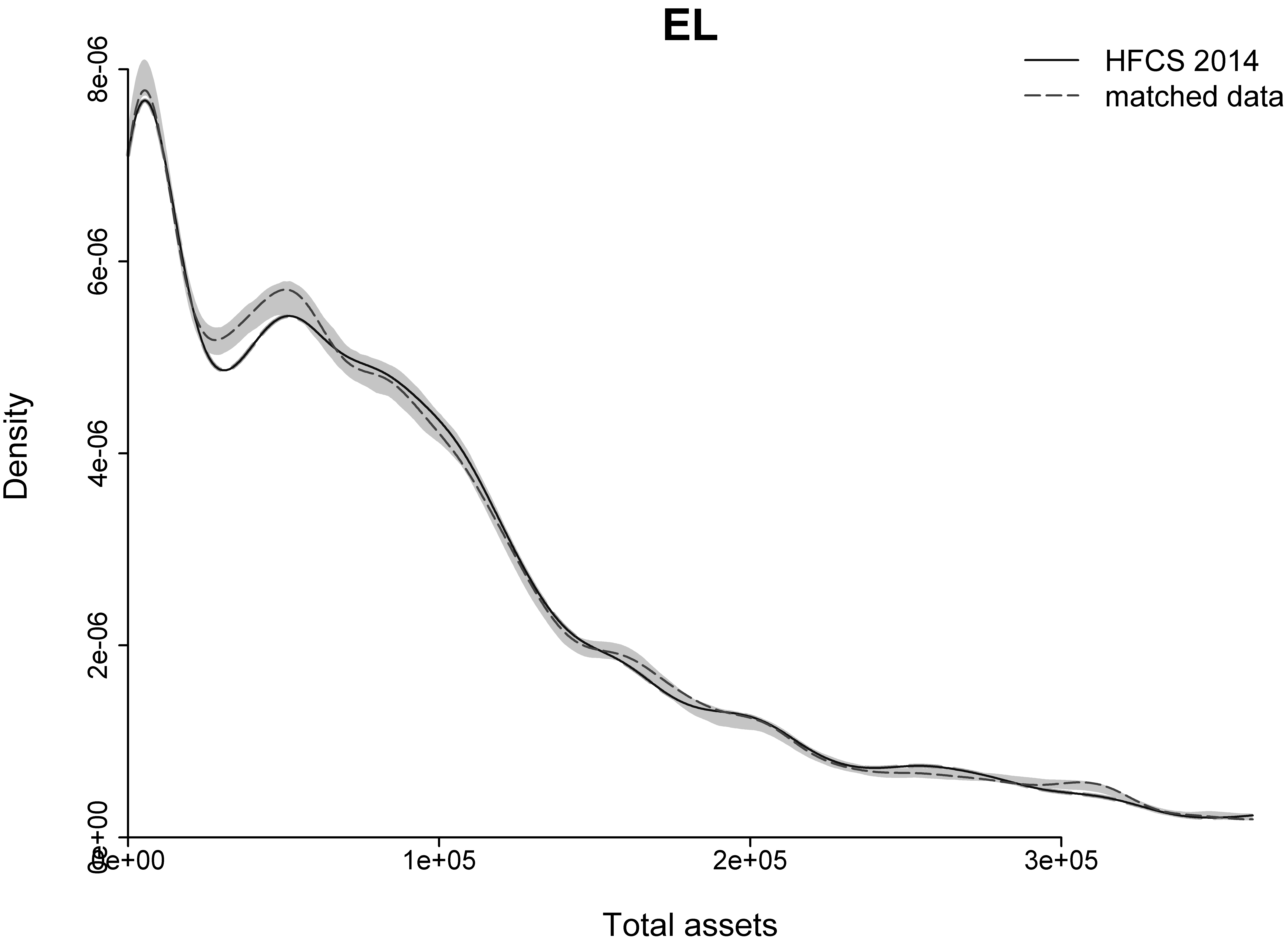
Likewise, Figs 4–6 show the comparison of total assets distribution in the HFCS and the matched SILC-HBS-HFCS data set. The probability density functions suggest that the matching of income-wealth data is slightly less reliable than results obtained for income-consumption. This is confirmed when comparing the gap between the cumulative distribution of total assets in the matched data set to the original data (Table 4): Some gaps seem very large, although often it is merely the relative difference in percent which is high whereas the absolute difference is minimal because the amount of total assets is very low. This is particularly true for differences in Q10 and Q25, i. e. the 10% or 25% of households with the lowest amount of assets.
Summary table of the gap (%) in the distribution of original HFCS total assets and total assets in the matched data set (2015)
Probability density function of total assets from original HFCS data and the matched data set for Latvia. The shaded area reflects the 95% confidence interval obtained from the 100 repetitions of the matching process. 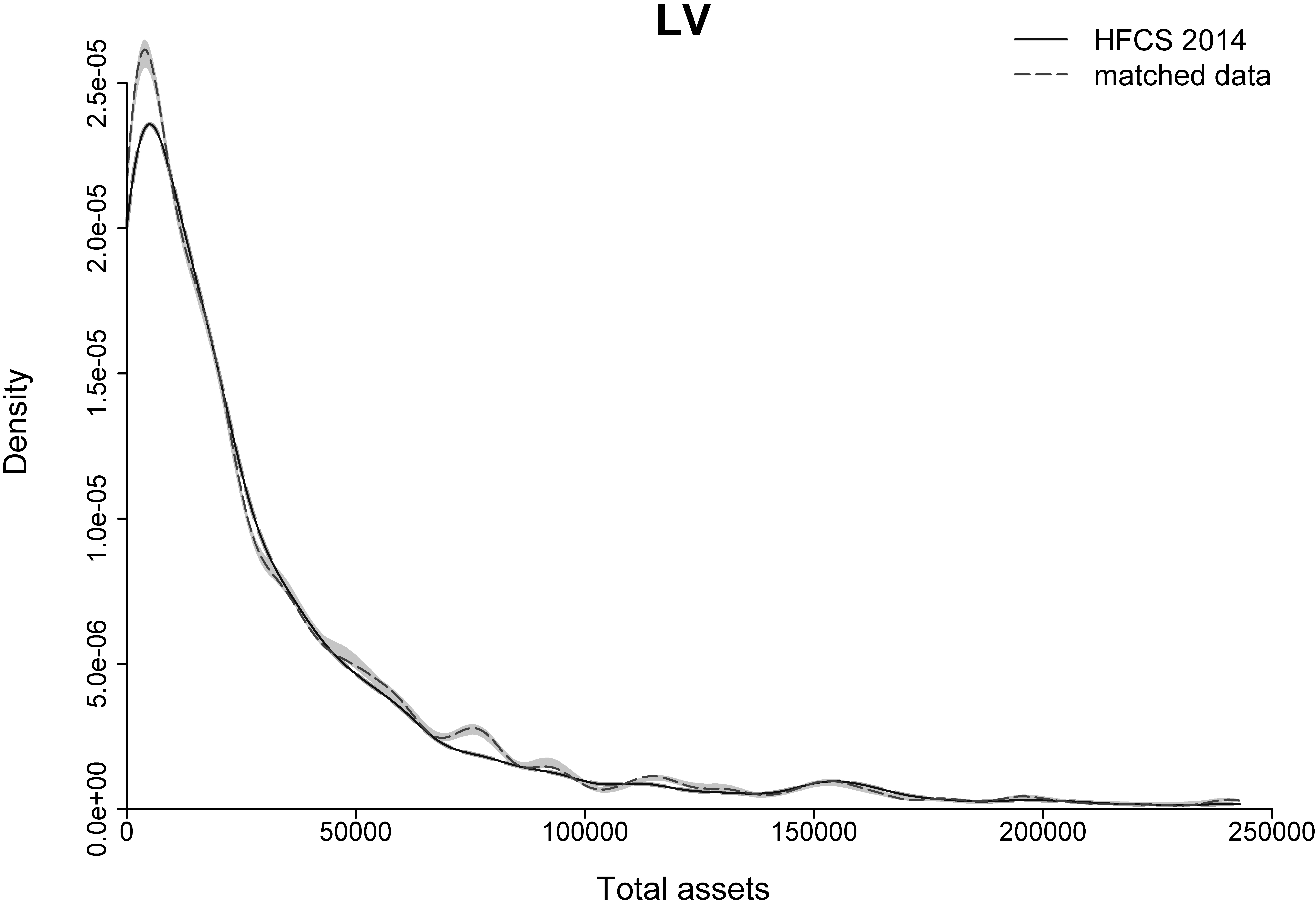
Correlations between income and consumption in the OCW module (EU-SILC 2017) and their partial correlation given 20-quantiles income
Correlations between income and wealth in the OCW module (EU-SILC 2017) and their partial correlation given gross income
An additional quality check is based on the use of an external source: the module on Over-indebtedness, Consumption and Wealth (OWC) of the 2017 EU-SILC wave, available for some countries. This module provides information on income and consumption, which allows computing their correlation given the 20-quantiles of income (Table 5). When we eliminate the effect of this matching variable from the correlation between income and consumption, the resulting correlations are dramatically reduced, being in most of the cases not significant anymore. This analysis shows the important role of the income quantiles in explaining that relationship. This approach is an assessment of the CIA which, based on the results obtained, can be considered as an approximate model between the two target variables.
Spearman correlation coefficients between consumption and the non-nominal matching variables in the original and synthetic data sets
Spearman correlation coefficients between wealth and gross income in the original and synthetic data set
With regard to the statistical matching of the SILC-HBS and the HFCS target variables, the OWC 2017 module also allows us to compare, for some countries, the correlations between income and wealth given the matching variable on gross income (Table 6). The reduction of the correlations when eliminating the effect of the gross income variable indicates the relevance of this matching variable in explaining the relationship between income and wealth as well as a verification of the CIA.
In yet another quality test, we analyse whether the association between the matching and the target variables observed in the original HBS and HFCS data sets are preserved in the synthetic data set (Tables 7 and 8). The comparison of the corresponding Spearman correlation coefficients for the synthetic data set with those correlations in the original data set, reveal similar correlation structures, both in strength and direction.
Note: Data for Italy were excluded from further analysis since the statistical matching did not produce convincing results. This is because the income quantiles could not be used as matching variable due to missing income data in the original HBS data set for Italy.
Share of households in bottom 20% of income, consumption and/or wealth
First, we look at households which belong to the 20% poorest in terms of income and consumption or in terms of income and wealth (total assets), and at the share of households which fall into the 20% poorest in all of the three dimensions (Table 9). Shares are highest for households with low income and consumption ranging between 15% in Czechia and Bulgaria to 10% in Greece and the Netherlands. 25% to 55% of the households with low income and consumption belong also to the 20% of households with the lowest amount of total assets.
Median consumption in thousand PPS by income decile. PPS 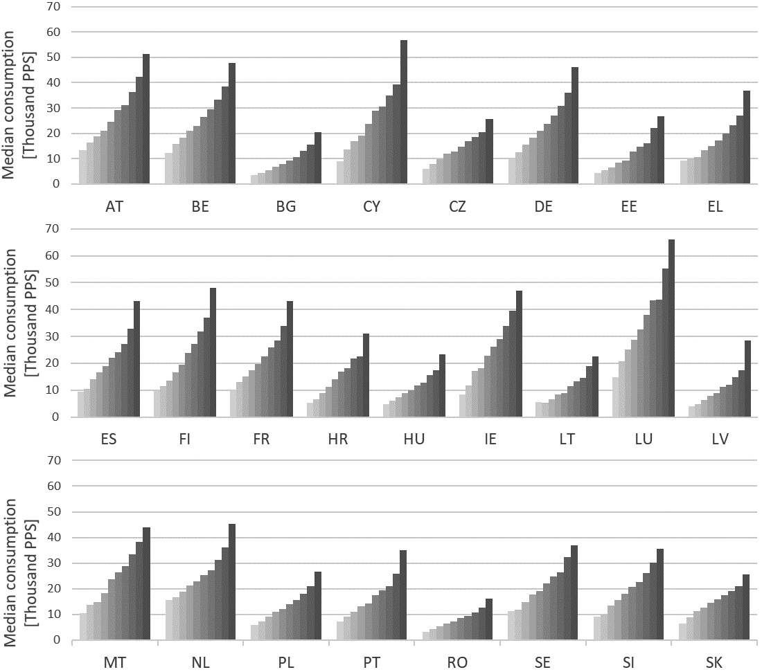
Share of households belonging to the 20% with lowest income and consumption (IC_Q1), lowest income and wealth (IW_Q1) and lowest income, consumption and wealth (total assets) (ICW_Q1) respectively
An obvious result of the matched income-consump-tion data set is the mean consumption of households by income deciles (Fig. 7). Using purchasing power standards (PPS) as a unit allows to compare the median consumption in different EU countries (although national deviations of the reference year 2015 should be taken into account). Since the matched SILC-HBS data set has been re-calibrated such that the household weights fit the margins of mean consumption in purchasing power standards (PPS) by income quintile (among others), this result is particularly consistent with original HBS data. On average, households in Luxembourg spend by far the most, followed by Austria and Cyprus. Some countries show particularly large differences in the consumption of households with low and high incomes. The ratio in median consumption between households in the highest to households in the lowest income decile is highest in Latvia, followed by Estonia, Cyprus and then Croatia.
Median saving rates (%), 2010 and 2015. 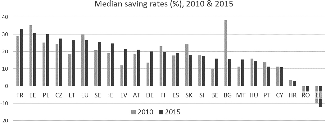
The matched income-consumption data set also enables us to calculate saving rates as a measure of the household’s capacity to set aside resources that might alleviate future income or consumption shocks, or be turned into assets on a longer term. We compute household saving rates as the difference of household disposable income and total consumption divided by disposable income:
Figure 8 shows the median saving rates of households for 25 out of the 27 EU countries (all except for DK and NL). In 2015, the median saving rates range between 33 and 11%, with the exception of Croatia, Romania and Greece with considerable lower median saving rates. In most countries, saving rates changed significantly from 2010 to 2015, with 13 out of 24 countries experiencing a positive change. Much more informative though are the differences in median saving rates between income quintiles. Figure 9 reveals the change in median saving rates between 2010 and 2015 for the 1
Change in median saving rates from 2010 to 2015 for the first and fifth income quintile.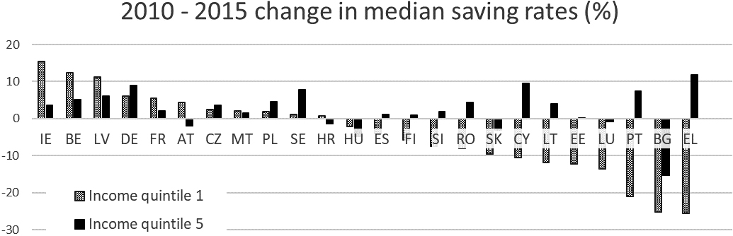
Inequality in disposable income, total consumption, savings and net wealth can also be looked at using Lorenz curves. Figures 10 and 11 show the Lorenz curve for 2015 data for Germany and Belgium. Inequality in savings is very high in both cases, and likewise for all other EU countries, although inequality in income and consumption on their own is much less pronounced. For some countries, like Belgium, inequality in savings even exceeds inequality in net wealth except for the very rich.
Lorenz curves for total disposable income, total consumption, savings and net wealth for Germany, 2013/2014. 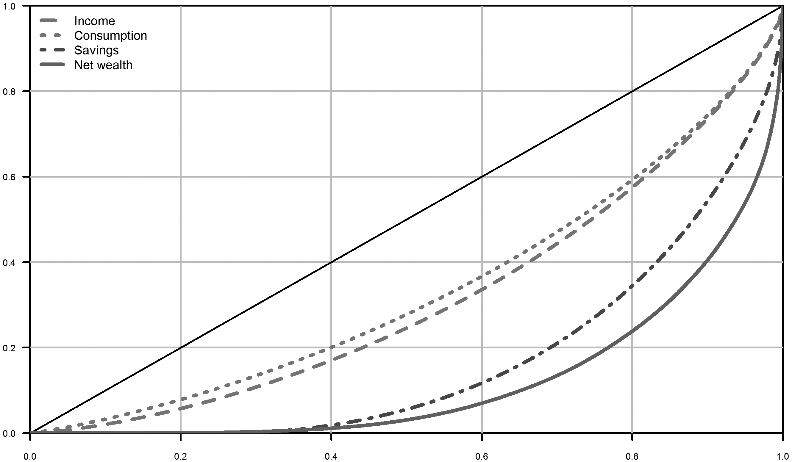
Lorenz curves for total disposable income, total consumption, savings and net wealth for Belgium, 2014.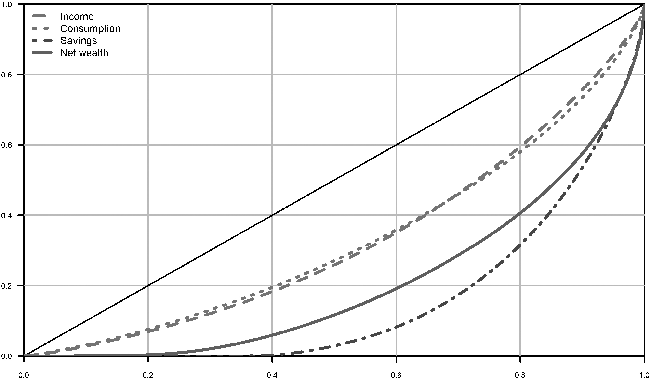
Finally, we look at asset-based vulnerability. We define a household at risk of asset-based vulnerability if the total assets of the household do not enable its members to stay above the AROP threshold for longer than a given period of time [3]. (The AROP threshold means that the equivalised disposable income of the household is below 60% of the national median equivalised disposable income). In other words, the time after which the total assets of the household will be used up, in the hypothetical event of the household ceasing to receive income and using its total assets to finance the needs of its members. Figure 12 shows this indicator for periods of one, three, six, nine or twelve months. From the 16 countries for which these data are available, Ireland, Germany and the Netherlands have the highest share of households having used up their total assets after one month already with 20% in Ireland and 17% in Germany and the Netherlands. Latvia and Finland follow closely with 16% each. 34% of households in Ireland and Germany and 32% in Austria have used up their assets after 12 months of no income.
Share of households at risk of asset based vulnerability (2015) meaning that the total assets of the household have been used up after one, three, six, nine or twelve months in the hypothetical event that no other income may be disposed of. 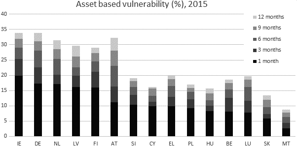
Quality of the matching
The comparison of probability density functions and cumulative distributions of the matched income-consumption-wealth data versus original data shows good results for most countries. Likewise, the correlations between income, consumption and wealth in the synthetic data set compare well with the correlations obtained through the OWC 2017 module. The similarity of the overall distributions, however, does not guarantee that individual households have been matched correctly. In some cases, the stratification used for the matching may lead to wrong assumptions of the household’s real consumption and/or wealth pattern. This is why conclusions for individual households or small subpopulations should not be drawn from the matched data set.
A likely reason why the comparison of original data with the matched data shows larger differences for total assets than for total consumption is the highly skewed distribution of wealth in most countries, making it much more difficult to explain wealth out of variables common to the different surveys. In economic terms, wealth may be seen as the result of a complex phenomenon at the household level, resulting from a series of decisions between consumption and savings, usually supported by anticipations and risk aversion, as well as exogenous lifetime events (inheritances, but also personal events such as unemployment, disease, separation). As a result, wealth comes with a very individual path for households, making it very difficult to valuate a “likely” wealth amount in absence of variables describing major events and worries of the individuals living in the household.
Income, consumption and wealth indicators
Once income, consumption and wealth are observed jointly at the household level, it is possible to draw different types of uses of this data set. The first kind of analysis consists naturally of understanding better the economic behaviours of households and explaining more comprehensively the dynamics of inequalities in the EU. Some examples of such indicators have been shown in the results part of this paper, although a variety of other indicators can likewise be produced based on the very variables used in the statistical matching. A second set of analyses comes swiftly to policy purposes regarding inequalities and more particularly fiscal policies. Having at one’s hand information at the micro-level on income, consumption and wealth makes it possible, at the cost of additional hypotheses, to describe in a comprehensive way the fiscal incidence for every household in the sample, by computing direct and indirect taxes. Subsequently, the impact of fiscal reforms may be evaluated taking into account the fiscal system as a whole.
Conclusions
Given the use of proxy variables, which are highly correlated to the target variables, the Conditional Independence Assumption allows us to obtain a joint distribution of income, consumption and wealth through the statistical matching of individual data sources.
The quality of the matching is limited, however, through the number of potential matching variables in the harmonised data sets available for all EU countries. It is further jeopardized through differences in reference years. Due to these reasons, indicators drawn out of this exercise should be interpreted cautiously in particular with regard to smaller subgroups of the household population.
Nevertheless, the exercise is highly relevant as it sets the scene for more integrated micro-data collections and recalls the importance of estimating joint distributions for key economic dimensions of the household sector. More reliable results could be achieved through a decentralized exercise in which national statistical institutes carry out the exercise themselves, using -in the most ideal situation- observed joint distributions (such as integrated surveys or matched administrative data) or, as a second-best solution, modular approaches and statistical matching techniques with variables that best fit the national context. A few countries have already taken this way.
Footnotes
The EU-SILC and HBS surveys are run by the National Statistical Institutes of the EU and coordinated centrally by Eurostat. The HFCS is run by the National Central Banks of the Euro area and coordinated by the European Central Bank. The results published in the present paper and the related observations and analysis may not correspond to results or analysis of the data producers.
EU-SILC and HBS 2015 data were available for all EU27 countries, but Denmark, in 2020. For 2010 the Netherlands are missing. HFCS 2015 data are available for all countries of the Euro area plus Poland and Hungary.
Income data are collected in the HBS survey through a limited number of questions resulting in a rough income variable, which is not comparable to disposable income in EU-SILC for most countries. Moreover, the income concept in HBS is not harmonised among countries.