DEBISim: A simulation pipeline for dual energy CT-based baggage inspection systems 1

Abstract

BACKGROUND:

Materials characterization made possible by dual energy CT (DECT) scanners is expected to considerably improve automatic detection of hazardous objects in checked and carry-on luggage at our airports. Training a computer to identify the hazardous items from DECT scans however implies training on a baggage dataset that can represent all the possible ways a threat item can packed inside a bag. Practically, however, generating such data is made challenging by the logistics (and the permissions) related to the handling of the hazardous materials.

OBJECTIVE:

The objective of this study is to present a software simulation pipeline that eliminates the need for a human to handle dangerous materials and that allows for virtually unlimited variability in the placement of such materials in a bag alongside benign materials.

METHODS:

In this paper, we present our DEBISim software pipeline that carries out an end-to-end simulation of a DECT scanner for virtual bags. The key highlights of DEBISim are: (i) A 3D user-interactive graphics editor for constructing a virtual 3D bag with manual placement of different types of objects in it; (ii) An automated virtual bag generation algorithm for creating randomized baggage datasets; (iii) An ability to spawn deformable sheets and liquid-filled containers in a virtual bag to represent plasticized and liquid explosives; and (iv) A GPU-based X-ray forward modelling block for spiral cone-beam scanners used in checked baggage screening.

RESULTS:

We have tested our simulator using two standard CT phantoms: the American College of Radiology (ACR) phantom and the NIST security screening phantom as well as on a set of reference materials representing commonly encountered items in checked baggage. For these phantoms, we have assessed the quality of the simulator by comparing the simulated data reconstructions with real CT scans of the same phantoms. The comparison shows that the material-specific properties as well as the CT artifacts in the scans generated by DEBISim are close to those produced by an actual scanner.

CONCLUSION:

DEBISim is an end-to-end simulation framework for rapidly generating X-ray baggage data for dual energy cone-beam scanners.

Keywords

X-ray based threat detection baggage security screening dual energy CT

1 Introduction

X-ray based baggage screening provides a fast and non-invasive means for the detection of hazardous and illicit materials in airport bags. Such inspection systems have therefore now become an integral part of airport checkpoint security, with CT scanners used for inspection of checked baggage and two-view projection imaging systems for screening carry-on bags. For these security imaging systems, it is common practice to subject the 2D and 3D scan images to rudimentary computer processing in order to highlight the image regions where the x-ray attenuation is even slightly above the norm for benign materials. Highlighting threat regions within the baggage scan facilitates rapid human examination for tagging the bags for manual inspection and hence improves the overall inspection time.

Obviously, the level of automation in these systems is rather low, with the human operator eventually deciding whether the screened bag is to be intercepted. To make sure that the human operator does not miss even the most primitive forms of explosives [1], the thresholds used to delineate the regions inside the baggage image must therefore be set sufficiently low. Setting a low threshold for delineation ensures that the system highlights even those regions and items within the baggage scan that have even the slightest chance of being hazardous. However, this makes for a high workload for the downstream human operators and also for a greater need for manual inspection of the bags.

This state of affairs has led to calls for using modern machine learning (ML) techniques for raising the level of automation in airport baggage inspection systems. The hope is that ML would go beyond just thresholding the image data on the basis of pixel- or voxel-based attenuation values for delineating the suspicious regions in a bag.

There are two approaches that one can take to develop ML-based techniques for threat detection: the first approach relies on using attenuation data from traditional single-energy X-ray imaging systems while the other method explores the use of dual-energy X-ray imaging to improve threat identification [2]. A fundamental limitation of the traditional imaging system is that the X-ray attenuation coefficient is not sufficient to discriminate between certain hazardous materials and those used for everyday applications. On the other hand, using two X-ray beams whose photons occupy two different energy bands allows not only for a more precise calculation of X-ray attenuation but can also extract additional material properties such as the effective atomic number for the scanned baggage volume [3]. Such dual energy scanning methods have exhibited proven capability in identifying the aforementioned “harder-to-discern” threat materials and therefore are believed to be better candidates for further automating airport baggage inspection. Furthermore, being able to estimate two different material properties opens up all kinds of new possibilities for baggage inspection and also the likelihood that some of them would allow for greater automation in baggage inspection through the use of ML.

That brings us to the main purpose of the work reported in this paper: facilitating ML research in the context of DECT imaging. Towards that end, it is important to note that all machine learning algorithms require positive and negative examples of the objects that the algorithms must discriminate. For airport baggage inspection, that means positive bags, i.e., bags with explosives in them, and negative bags without any hazardous contents. For an ML algorithm to be robust, these positive and negative training examples must capture all of the real-life diversity in both kinds of bags. Whereas it is relatively straightforward to generate such training data in many more routine applications of ML, that is not the case for baggage inspection.

Generating positive training examples for baggage inspection not only requires handling explosives, but also anticipating the different possible ways in which an adversary may pack a bag with explosives in order to hide their presence amongst the baggage contents. These two challenges make it very difficult to create the needed positive examples.

We believe these difficulties in creating a sufficiently large number of positive examples needed for ML algorithms can be addressed with a simulated data generation framework. There already exist several open source X-ray simulators that accurately capture the physics of X-ray beam interactions in terms of the absorption, scatter, and diffraction of the photons. By combining such a software library with one that accurately models the structure and contents of a generic airport bag, it is possible to a create a fully end-to-end automated software pipeline that can generate with high precision the kind of data that a real scanner would for the bag. Presentation of this pipeline is the goal of our paper.

In this paper, we present DEBISim (Dual Energy Baggage Image Simulator), a software for creating virtual 3D bags and producing the same kind of data and images for the virtual bag that a real DECT scanner would do for a real bag.

With regard to how a virtual bag is created, DEBISim can be used in the following two modes:

Manual Mode: In this mode, a user is provided with an easy-to-use 3D graphics editor that allows the user to first define the shape and the materials for the objects to be placed in the bag, and then a set of controls for placing, scaling, orienting each object within the bag. The virtual bag generator also allows the user to place custom complex shapes and liquid-filled containers (for liquid explosives) in the bag.

Automatic Mode: DEBISim uses a randomization algorithm to pack a bag with a random assortment of shapes, sizes, and materials. The objects placed in a bag are subject to the rules of gravity which does not allow for the objects to be free floating. The randomly generated objects also include deformable sheets (for sheet explosives) and liquid filled containers in addition to the bulk and complex shape objects mentioned above for the manual mode.

The virtual baggage volume is then scanned with a simulated helical-scan cone-beam scanner which is a commonly used scanner geometry for baggage inspection. For projection data generation, the users can set the parameters for the scanner geometry as well as for the energy spectra of the X-ray source(s).

The dual-energy projections are then subjected to a dual-energy decomposition that yields line integrals of the Compton and the Photoelectric coefficients. Subsequently, the values obtained for such line integrals can be processed to reconstruct the 3D coefficient images for the respective parameters, or projected into an alternative feature space that lends itself better to the calculation of the effective atomic number and the attenuation coefficient in each voxel. A user can choose from a number of dual-energy decomposition methods including one of our own formulations [2 , 5].

Finally, the DEBISim pipeline also includes a standard suite of helical-scan cone-beam reconstruction algorithms for 3D reconstructions of a virtual bag. This allows an ML researcher to experiment either directly with the sinograms for classifying a bag or with the 3D image data.

We have tested DEBISim using two standard CT phantoms: the American College of Radiology (ACR) phantom [6] and the ANSI N42.45-2011 Standard Security Screening phantom [7]. This comparison study involved first constructing virtual models of those phantoms using DEBISim and then simulating the corresponding projections and 3D reconstructions for the simulated phantoms. The reconstructions were then compared with the corresponding real scans of the phantoms obtained from the same spiral cone-beam scanner that was modeled in DEBISim. Since the material properties of the different parts of these phantoms are known precisely, a direct comparison of the real and simulated scans yields a check on all three aspects of the simulator: 3D modeling, dual-energy projection data generation and dual-energy decomposition, and, finally, reconstructing the 3D images of the phantoms. In a similar manner, we have also tested the simulator performance for a set of reference materials that represent the type and range of materials frequently encountered in checked bags. The comparative analysis with the real scans for all these cases shows good replication of material-specific properties and the CT artifacts in the simulated data.

The organization of the paper is as follows: Section 2 provides an overview of the currently available CT simulators that can be used to synthesize data for threat detection. It also reviews the efficacy of these simulators for ATR system design. Section 3 describes in detail the baggage simulation pipeline for DEBISim along with each of its four functional blocks. It also describes how the DEBISim pipeline operates for automated and manual data generation. Section 4 presents the implementation of each of the functional blocks and sub-blocks. Lastly, Section 5 shows how we validated DEBISim using the ACR and ANSI standard phantoms as well as on a set of reference materials. The paper concludes by illustrating simulation examples of the different datasets generated by DEBISim for ATR system design.

2 Relevant literature

There exist several X-ray simulators that can simulate with high-quality the more traditional CT scanners with different geometries [8 –10]. Again for the more traditional forms of inspection, simulators like PRISM [11] have been developed specifically for checked baggage under the assumption that a bag lends itself to CAD modeling. Such simulators employ physics engines such as Geant4 [9] or Penelope-2014 [12] for X-ray simulation. These engines use Monte Carlo logic to estimate the photon flux incident on the detectors as well as its atomic interactions with the scanned volume. While the Monte Carlo simulation based methods can accurately emulate even higher order scattering effects for X-ray transmission, it is at a cost of high computation time and memory.

A second class of X-ray simulators are the ones that use deterministic ray tracing (DRT) for estimating X-ray interactions. While the simulations obtained using this approach do not have as high a degree of accuracy as the Monte Carlo based methods, the DRT approach can still estimate X-ray photoelectric interactions well while requiring much less time for computation. As a result, many simulators have adopted this approach for rapid simulation of X-ray scans. For example, Gong et al. [13] use DRT for estimating projection data for two-view X-ray baggage scanners from a 3D mesh model of a bag. The most recent such contribution based on DRT is the QSim framework [14, 15] that incorporates GPU support for ray tracing and that can generate synthetic X-ray data for complex baggage models. The DEBISim simulation pipeline proposed in this paper also uses deterministic modeling for fast simulation of baggage CT scans. As far as the scattering simulation is concerned, it can be approximated in DEBISim by adjusting the DC offset gain for the projections to match the observed background scatter.

Most of the simulators that have been reported in the literature do not lend themselves to the modeling of dual-energy scanners for baggage inspection. Additionally, the automation support they provide for creating virtual bags is less than adequate — especially considering the ground-truth data needs of modern machine-learning algorithms. Both these points have been addressed and incorporated in the DEBISim simulation pipeline. Thus, DEBISim provides an end-to-end framework for baggage simulation that makes it easy for a user to configure the contents of a virtual bag to manually and automatically generate training and testing data for developing ML algorithm for explosives detection in bags.

3 An overview of the DEBISim pipeline

This section presents at a rather high level the architecture of the DEBISim simulation pipeline. It also presents the two modes of operation used for virtual bag creation, i.e., the manual and automatic modes.

3.1 The DEBISim simulation pipeline

The functional block diagram of the DEBISim simulation pipeline is shown in Fig. 1 along with its input specifications and outputs at different stages of the pipeline. As shown in the figure, the simulator consists of a modular pipeline with four basic building blocks: (i) the Virtual Bag Generator, (ii) the X-ray Forward Modelling Block, (iii) the Dual Energy Decomposition Block and (iv) the Reconstructor block.

Fig. 1

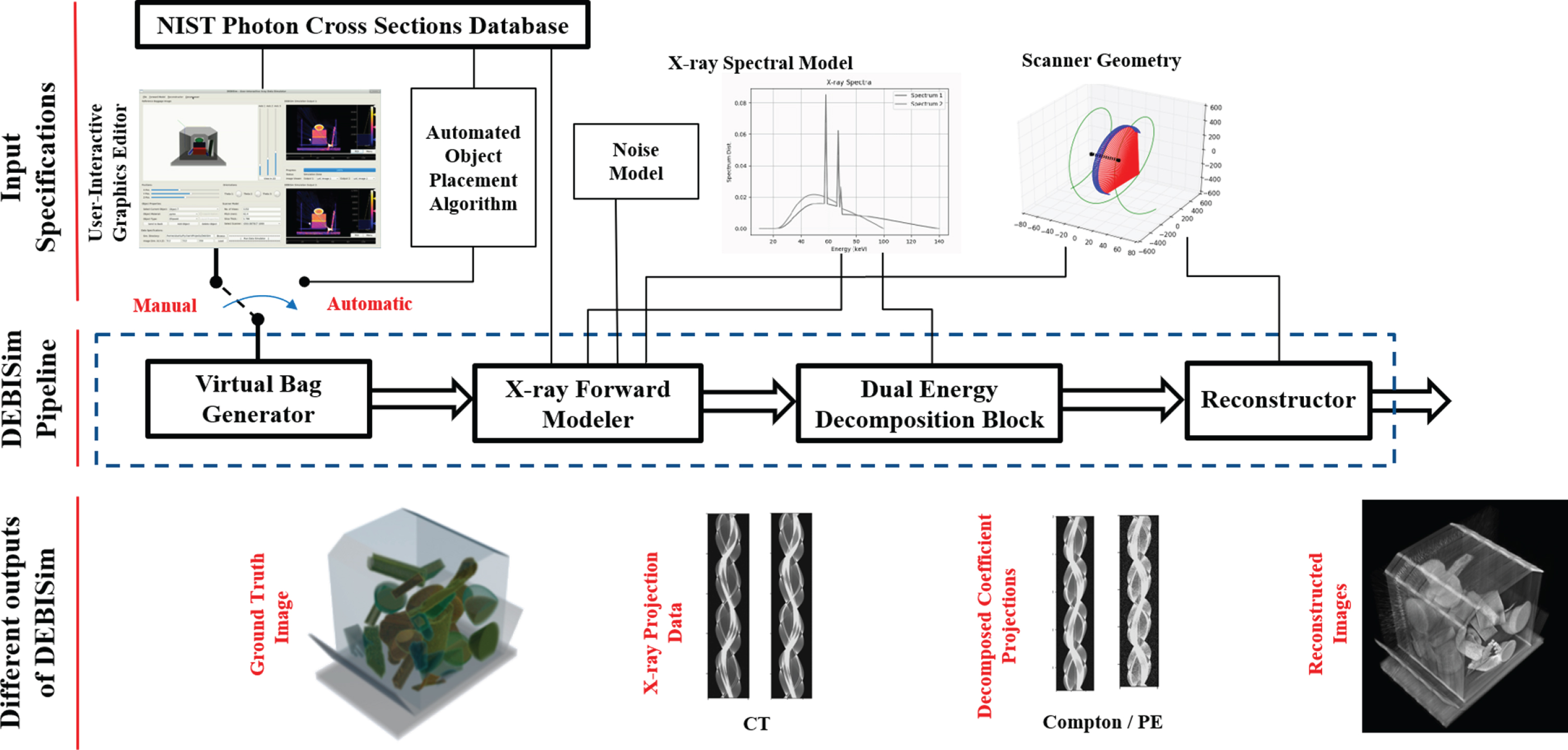
DEBISim Simulation Pipeline: As shown, the pipeline consists of the following four blocks: (i) Virtual Bag Generator, (ii) X-ray Forward Modeler, (iii) the DE Decomposition Block and (iv) the Reconstructor. The Virtual Bag Generator operates differently for the manual and automatic modes as described in Section 3.2. The X-ray Forward Modeler employs the knowledge of the scanner geometry, X-ray source spectra, and CT noise models to generate the projection data for a bag. The DE Decomposition and Reconstructor blocks can select from a number of options for processing/reconstructing the X-ray data.

Ordinarily, one would want to use all the four blocks shown in Fig. 1 for generating the projection data and for reconstructing images from the data for a given virtual bag. But it is also possible to use the blocks individually or in combinations for more specialized applications of the simulator. For example, just the last two blocks can be used to reconstruct images from the dual energy projection data generated by a real scanner. To cite a specific example of this more specialized application of the simulator, we have used DEBISim to create a dataset for MAR (Metal Artifact Reduction) analysis by running the last three blocks twice – one for the original virtual bag and one for the virtual bag with all metal objects removed.

The subsections that follow provide a brief description of the functionality provided by each of the four blocks.

3.1.1 Virtual bag generator block

This block generates a virtual volumetric bag that contains user-specified objects with user-specified shapes and material properties. Virtual bags can be generated either in a user-interactive manual mode or automatically through a randomized procedure. In the user-interactive mode, a virtual bag can be manually generated by packing different objects in it using the DEBISim GUI. In the automatic mode, an automated bag-packing algorithm generates a randomized bag that can be run iteratively to produce a randomized baggage dataset for an ML algorithm. Note that even when the bags are generated automatically, their properties, such as the list of materials to select from and their shapes, can be set by the user.

3.1.2 X-ray forward modelling block

The X-ray forward modelling block generates the projections of a virtual bag for the imaging geometry defined for a spiral cone-beam scanner. The DEBISim interface makes it easy to configure the scanner specifications so that they correspond to a real scanner. Taking into account the user-specified scanner geometry, DEBISim employs the ASTRA toolbox [8] for generating the projection data for one or more X-ray spectra representing the CT sources (See Fig. 1).

3.1.3 Dual energy decomposition block

This block is used for processing the dual energy CT projections generated by the forward modelling block in order to extract the DECT coefficient line integrals [3]. Depending on the basis functions used for DECT decomposition, the line integrals correspond to different pairs of material properties. For example, a commonly used pair is that of the Compton and Photoelectric Coefficients [2].

3.1.4 Reconstructor block

This block generates the 3D CT reconstructions. The reconstruction algorithms can be applied either directly to the dual-energy projection data as returned by the Forward Modeling Block as well as to the line integrals returned by the Dual Energy Decomposition Block. The reconstruction parameters in the algorithms are derived from the scanner geometry defined in the X-ray forward modelling block. The reconstructed CT data can be visualized on-the-go.

3.2 About the two modes of operation of DEBISim

As mentioned earlier, DEBISim can be operated in the following two different modes:

3.2.1 Automatic virtual bag generation

In this mode, the simulator generates a specified number of bags by randomizing a set of object property parameters. More specifically, automated bag generation is done by iterating the DEBISim pipeline for each bag while randomly generating and placing a set of objects with randomly assigned material properties in the bag. The simulator uses heuristics for deciding where to place a new object in the bag. This is followed by a placement optimization operation which fine-tunes the placement of the object. Both the heuristics and the optimization operation ensure that no objects in the bag are free-floating. The placement of the baggage contents is best visualized as a human “dropping” each object in the bag and the object coming to rest in position and orientation that depends on the spatial configuration of the objects previously placed in the bag. For the placement logic to work correctly, the objects are assumed to be rigid. DEBISim also allows for packing deformable sheets in a bag for representing sheet-like plasticized explosives like PETN and Semtex. Sheet deformation takes place automatically upon placing the sheet within the virtual bag by means of a sheet placement algorithm. Finally, DEBISim can also instantiate liquid filled containers for placement in a bag. These are for representing liquid explosives such as nitroglycerin and ANFO [16]. Such containers may be filled to any desired level. The liquid levels are specified after the container has been placed in its final position and orientation in a virtual bag. This gets around the problem of having to change the fill level of the liquid as the container is subject to various translations and rotations for optimum placement in a bag, as explained in the next section.

3.2.2 User-interactive manual bag generation

Baggage configurations can also be manually generated using DEBISim with the help of a 3D user-interactive graphics editor. The GUI allows a user to interactively pack a virtual bag with objects of different shapes and composed of different types of materials. The user can select from a library of primitive shapes directly and the selected shape can be scaled up (or down) in size before being deposited in the bag. Additionally, complex custom shapes can also be loaded from 3D image files and packed in a virtual bag. After an object is given a shape and a size, it is translated and rotated as required. Subsequently, the object is assigned a material label whose X-ray transmission properties are calculated using the NIST Photon Cross Section Database [17]. An important feature of the DEBISim GUI is that it allows for new materials (natural elements, compounds, and mixtures) to be added to the existing list. Another feature of the GUI is the ability to modify the forward model specifications as per one’s own scanner setup.

4 Implementation details

This section presents at a deeper level the logic that goes into the various blocks of the DEBISim pipeline presented in the previous section. Although all the four major blocks of the pipeline are equally important, in what follows we devote a proportionately larger space to the 3D modeling of virtual bags since that is the most novel part of the overall pipeline. The computationally efficient approach that we present for generating bags breaks new ground in the space of creating fully virtualized sources of training and testing data for modern ML algorithms. We will also present further information about the three blocks. These blocks are a combination of our extensions to well-known modules in the open-source community and our algorithms for dual-energy decomposition.

In what follows, in Sections 4.1 and 4.2, we present first the automatic mode for virtual bag generation and then the manual mode. Section 4.3 then describes the X-ray forward modelling block that produces the simulated projections for the virtual bag. In Section 4.4, we take up the subject of dual-energy decomposition needed by the simulator. Finally, Section 4.5 mentions how the 3D images are reconstructed from the projection data in DEBISim.

4.1 Virtual bag generation – the automatic mode

As mentioned earlier, the automatic mode in DEBISim involves iterating through the simulation pipeline for each bag while randomly generating and placing a new set of objects within the bag with randomly assigned material properties. The material properties that are changed for every bag and its contents are selected from a set specified by the user. This allows the simulator to create randomized baggage datasets as needed by machine learning algorithms for their training. The simulator places each object in a bag by using a bag-packing algorithm that mimics a human letting go of the object as it is being placed in the bag and the object “settling” itself over the previously placed contents in the bag.

The automatic mode can spawn three types of objects in a virtual bag: (a) bulk objects – this class denotes rigid 3D objects whose shapes may either be primitive (cuboids, ellipsoids, cylinders, etc.) or complex, the latter including voxelized 3D representations of real objects such as cups, mallets, bottles, etc.; (b) deformable sheet objects – this type represents thin membrane-like objects that mimic plastic sheets or cloth that can stretch and deform when placed in a bag over other objects; and (c) liquid-filled containers – this type denotes those bulk objects that are hollow and hold liquids.

The upcoming three subsections of this section are devoted to each of these three types of objects. Note that the instantiation and placement logic for the bulk objects are also used for the liquid containers since, except for their hollowness, they are the same.

At a high level of description, the overall pseudo-code for automatic bag packing is described in Algorithm 1.

Algorithm 1 Bag-Packing Algorithm:

Packs an empty virtual bag with a set of objects O = {O⁽ⁱ⁾|i = 1, 2, 3, … N} that includes primitive/complex shapes, sheets and liquid-filled containers. Each object is randomly initialized with a poseO⁽ⁱ⁾ .x, a shapeO⁽ⁱ⁾ .shape, a material labelO⁽ⁱ⁾ .material and a flagO_i .liquid_flag denoting if it should be a liquid-filled container.

1. Initialize object set, O = {O⁽ⁱ⁾|i = 1, 2, 3, … N}.

2. Initialize a Baggage Occupancy Map B for an empty bag using Eq. 1.

3. for every object, O⁽ⁱ⁾ ∈ Odo

4. x_heur⟵ Apply Heuristic Packing Rules to O⁽ⁱ⁾// Section 4.1.1

5. ifO⁽ⁱ⁾ is a sheet do

6. Place deformable sheet O⁽ⁱ⁾ using Algorithm 2 // Section 4.1.2

7. else

8. O⁽ⁱ⁾ . x⟵Run placement optimizer, P (O⁽ⁱ⁾, x_heur, B) // Section 4.1.1

9. Update Occupancy Map, B with new object O⁽ⁱ⁾.

10. end

11. ifO⁽ⁱ⁾ . liquid _ flag is set do

12. Convert O⁽ⁱ⁾ to a liquid-filled container // Section 4.1.3

13. end

14. end

4.1.1 Instantiating and placing bulk objects

A virtual bag is a rectanguloid whose dimensions are chosen randomly at the time of bag generation from the size ranges specified by the user. Instantiation of a bag is followed by the instantiation of the objects that go into the bag.

The primitive shapes for automatic instantiation of bulk objects are cuboids, ellipsoids, cylinders and truncated cones. DEBISim also allows for automatic generation complex shapes. These complex shapes can include 3D voxelized representations of real-life objects which can be loaded into DEBISim using 3D image files. Examples of both primitive and complex shapes are illustrated in Fig. 2. The complex shapes shown in Fig. 2 were obtained from image files that contain 3D binary voxel masks for several different everyday objects scanned for the TO-4 CT dataset [18].

Fig. 2

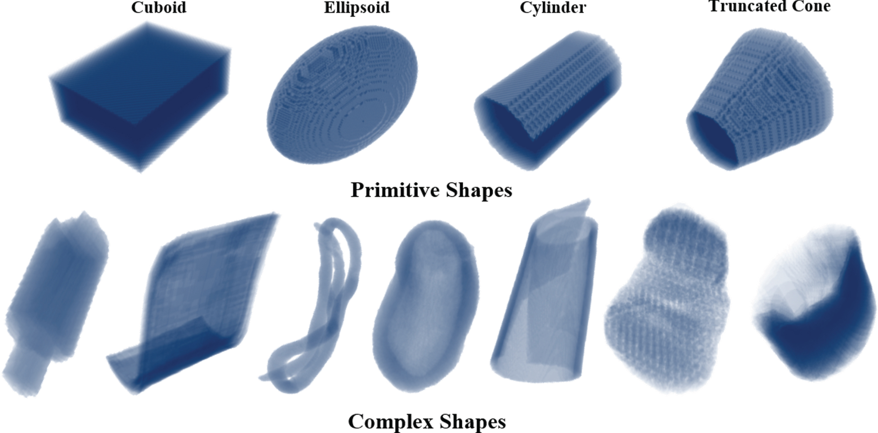
Bulk objects simulated in DEBISim: The figure shows examples of bulk objects that DEBISim simulates and packs in a virtual bag – these include primitive shapes (cuboids, ellipsoids, cylinders and truncated cones) shown in the top row of the figure as well as complex shapes shown in the bottom row.

Each primitive or complex 3D shape is defined with a “standard pose” and “standard size” in its own coordinate frame. The user can specify the subset of all available shapes to be used when the bags are generated automatically. By default, a random selection is made from all available primitive and complex shapes. After a bulk shape is instantiated, it is resized in a randomized manner. For complex shapes, the object is resized with a randomly assigned scaling factor. For the case of cuboids and ellipsoids, the object is resized by randomly scaling the lengths of their three principal axes. For cylinders and cones, it is the radii and the axial lengths that are scaled.

Subsequently, the resized object must be placed in the bag. The placement logic for bulk objects involves the following two steps: (1) DEBISim first applies two heuristic rules to an instantiated object to bring it as close to the bottom of the bag as possible. And (2) DEBISim manipulates the object in the vicinity of where it landed through the first step in order to eliminate what would otherwise be untenable object poses. Each of these two steps is described in detail in what follows.

Heuristic Packing Rules:

As shown in Algorithm 1, these rules are applied to all objects created for placement in a virtual bag. These rules are based on the following two general heuristics for object placement: (i) At no point during the placement process should there be any overlap between the volume occupied by the new object and the objects already in the bag or the bag boundaries; and (ii) The objects are placed in a bottom-up manner so that each new object settles as close to the bottom of the bag as possible.

An example of these heuristic packing rules in action is illustrated in Fig. 3. Step 1 in Fig. 3 shows the initialization of a new object (the cyan circle) at a random location within the unoccupied space in the virtual bag. Step 2 shows the heuristic for placing the object as close as possible to the bottom of the bag. And, Step 3 shows the final placement for the object achieved by iterative applications of the heuristic so that there can be no overlap between a new object and those already in the bag or the bag boundaries. Should any overlap be detected, the movement of the object that caused the overlap is reversed and alternative directions tried for the next location of the object closer to the bottom. When all alternatives fail, that becomes the position at which the optimization described in the next section is applied.

The two packing rules all by themselves can result in untenable placements for the objects in a bag. As to why that would be the case, assume that the next object to be placed in a bag is a randomly generated rod, that is, a rod initialized with a random location and orientation within the bag. Applying only the two heuristics to this object could result in a packed bag as shown in the top row of Fig. 4a, which is not a tenable configuration for the objects in the bag.

A reader might think that we could get around this problem by instantiating all new objects in some standard pose that would make their placement through the two rules inherently stable. Unfortunately, such a stability cannot be guaranteed because it is dependent on the objects already present in the bag. That is, even if the random object generator instantiates a rod with its axis parallel to the bottom of the bag, when it is placed in the bag with only the help of the two heuristics mentioned above, you could end up with the situation shown in the top row of Fig. 4b, which would again be unacceptable.

We have therefore chosen to allow for the object instantiation logic to be random with respect all of the degrees of freedom associated with the object and to then get around the problem of untenable object placements by invoking the optimization logic presented next. The bottom rows in Fig. 4a and Fig. 4b show how the optimization logic to be presented next transforms the output of the two heuristic rules presented above to tenable object configurations.

Object Placement Optimization:

The placement of every bag that has been subject to the two heuristics in Part I is further fine-tuned with the optimization logic presented here in order to eliminate the untenable placement configurations.

The placement variables for an object O within the volume of a bag are its translation and rotation parameters $x = {[\begin{matrix} x & y & z & θ_{x} & θ_{y} & θ_{z} \end{matrix}]}^{T}$ . To calculate the placement cost f (x) for the placement variable, we first define a binary occupancy map function [19] for the bag and its current contents:

$B (x, y, z) = {\begin{matrix} 1, & for the currently occupied volume and the bag exterior \\ - 1 / | | y - y_{0} | |^{2} & for the vacant space within the bag \end{matrix}$ (1) where y - y₀ denotes the distance from the bottom of the bag which is assumed to be located at y₀. We assume that a bag is a 3D rectangular object whose primary surfaces are aligned with the principal coordinate planes of an (x, y, z) coordinate frame. The top and the bottom of the bag are set to be perpendicular to the y-axis. Figure 5a illustrates the idea of an occupancy map for placement optimization.

An object O being placed in a bag is also assigned an occupancy map function O′ (x) that can be translated and rotated through the six components of the vector x. With these two occupancy maps, any overlap between a new object O and the current contents of the bag (along with its boundary) can be checked through the Hadamard product, C, of the two maps: C = Bgreaterthangreaterthan ⊙ greaterthangreaterthanO′ (x). The overlap condition is thus determined by checking for any positive elements in C: $D_{overlap} = any ({c_{i} | c_{i} \in C} > 0)$ (2) The placement cost f (x) is then calculated as: $f (x) = {\begin{matrix} \sum_{c_{i} \in C} step (c_{i}), & if there exists overlap (i . e, Doverlap is True) \\ \frac{1}{| C |} \sum_{c_{i} \in C} c_{i} & if there is no overlap \end{matrix}$ (3) where step (·) denotes the unit step function that filters only the positive values in C.

To help the reader understand the nature of the cost function f (x), let’s focus on the orange rod shown in the middle figure in the top row in Fig. 4a. That rod was placed there by the application of the two heuristics in Part I. At the position where rod is shown in the figure, it has no overlap with any other objects or with the boundary of the bag. Therefore, the value of D_overlap will be false. In this case, f (x) is given by the second formula shown in Eq. (3). That is, f (x) is a summation of the elements of the Hadamard product of the two occupancy maps. Each element of this Hadamard product is the value of B at the points that correspond to those occupied by the orange rod. These values of B are equal to the negative inverse square-distances from the bottom of the bag. With discretized representations, if we associate a unit mass with each cell of the object occupancy map, we can interpret f (x) as the gravitational pull on the rod toward the bottom of the bag. As the reader will see, applying the placement optimization logic to this cost function would re-position the rod as shown in the lower-middle depiction in Fig. 4a.

In general, the cost function in Eq. 3 achieves two goals: (1) When there is overlap between the new object and the objects currently in the bag, the cost denotes the extent of the overlap in terms of the number of overlapping voxels. And (2) When there is no overlap, f (x) is equivalent to the gravitational pull on the object’s center of mass.

The optimum value of x for object placement is determined by:

$x^{*} = x_{heur} + \underset{x}{arg min} f (x) subj . to x_{1, 2, 3} \in [- L / 2, + L / 2], x_{4, 5, 6} \in [- \frac{π}{2}, \frac{π}{2}]$ (4) where x_heur is the initial value obtained from the heuristic packing rules and the search bound L for each of the translational coordinates determined by the largest dimension of the object as will be explained shortly. The reason for using the same bound for all three translational coordinates is that, for the sake of computational efficiency, we want position optimization to be carried out only in the local vicinity of where the object landed after the application of the heuristic rules in Part 1. Even under a limited search for the optimum placement of the object, there will, in general, be several values for x that would minimize the value of the cost function.

To illustrate the presence of these local minima in the cost function, consider the example represented by the dashed yellow rectangle that is shown in Step 3 of Fig. 3. That object landed in the position shown through the application of the two heuristic packing rules of Part I. As far as the cost function is concerned, that object in an equilibrium position, but it is only a local minimum for f (x) since the rectangle can be more optimally placed at the bottom right hand corner in a vertical alignment.

To get around the problems created by such local minima, we have chosen the following two step approach for finding the best final configuration for each new object that is placed in a bag. The approach consists of first applying what we call a global optimization strategy that broadly searches in the unoccupied regions of a bag with respect to all six components of x where the value of f (x) can be less than its current value. Subsequently, a more refined local search is conducted for finding the best resting place for the object.

Global Optimizer: We use the PSO (Particle Swarm Optimization) strategy for the global optimizer [20], mainly because the global search in PSO can be conveniently parallelized to boost the optimization speed. PSO involves randomly spawning a set of candidate solutions or "particles" in the search space whose “velocities” are updated iteratively according to the local best position from the particle’s history and the global best position of the particle swarm. By tuning the hyperparameters associated with the velocity updates, all the particles ideally converge to the global best position. As mentioned previously, for faster convergence of the particle velocities, the spatial search space for the optimizer is reduced to the extents [- L/2, + L/2] instead of the entire baggage volume. See the Appendix for further details on the PSO search strategy used in DEBISim.

Local Optimizer: Once a candidate point is chosen by the global optimizer, local optimization is done using a conjugate gradient algorithm [21] to fine-tune the solution. The Jacobian for the conjugate gradient algorithm is calculated analytically with the help of rotational transforms for the translation and orientation parameters in x [22] while search bounds for x are the same as those for the global optimizer.

An illustration of a virtual bag simulated with and without the placement optimization step is shown in Fig. 5b which eliminates what would otherwise be "floating" objects in a bag without increasing computation time significantly. The placement optimization algorithm is applied to all objects placed in the bag except for deformable sheets which have their own logic for placement.

Fig. 3

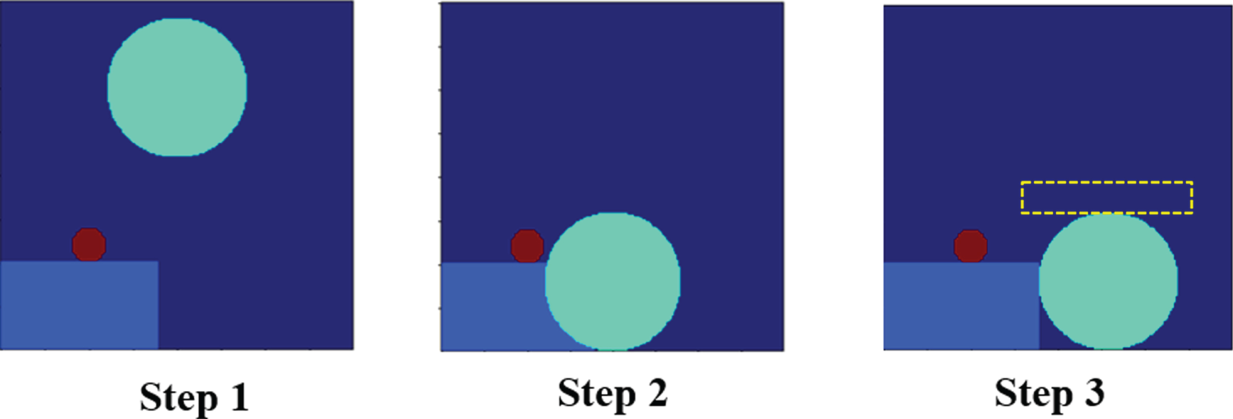
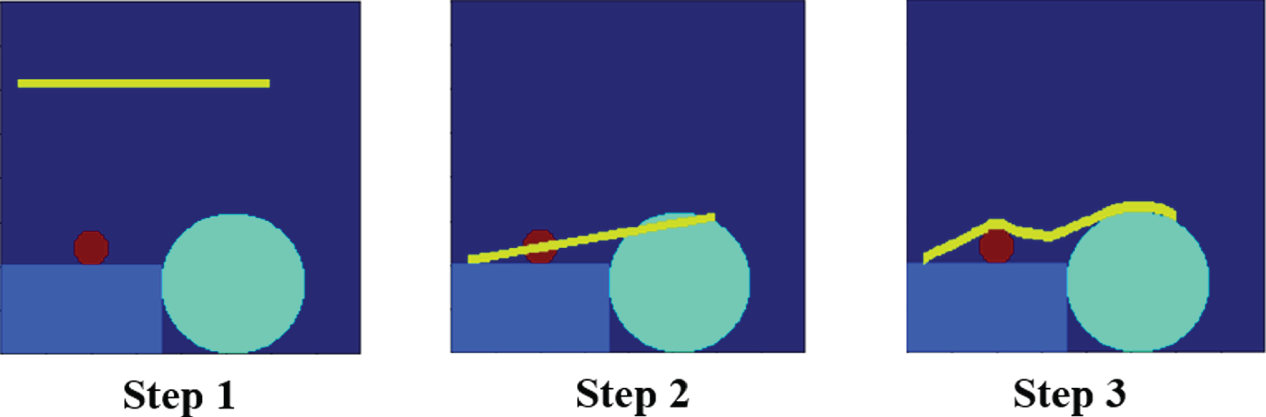
Heuristic Packing Rules: An example showing how the packing heuristics are invoked for a new object instantiated into the bag. Step 1 illustrates the current object (cyan circle) as it is randomly initialized in the bag. Step 2 shows the heuristic rules being applied to the object for bottom-up placement while Step 3 shows how the object position is adjusted to avoid inter-object overlaps. The dashed yellow rectangle illustrates the need for placement optimization as explained in Section 4.1.1.

Fig. 4

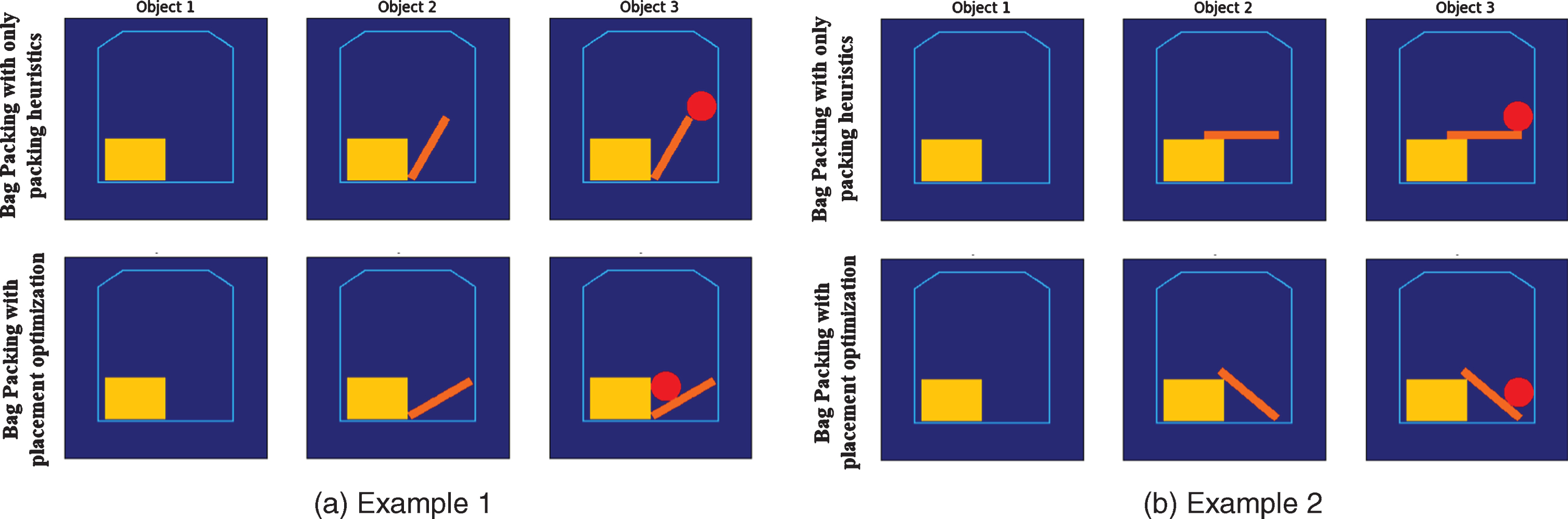
Need for Placement Optimization: This figure illustrates how using only the two packing heuristics for object placement, as presented in Part 1 of Section 4.1.1, can result in untenable baggage configurations. The top row in (a) shows three objects being placed consecutively in a virtual bag, with each object subject to just the two heuristics under the assumption that randomization is carried out with respect to all the degrees of freedom associated with each object. The orientation of the rod in the middle image in the top row in (a) is obviously untenable. The top row in (b) shows that one again ends up with unacceptable object configurations even if the objects are instantiated in some “standard” pose that one might think are less likely to result in the floating object phenomenon. The bottom rows in both (a) and (b) shows how the placement optimization logic transforms the otherwise unacceptable object configurations into tenable configurations.

Fig. 5

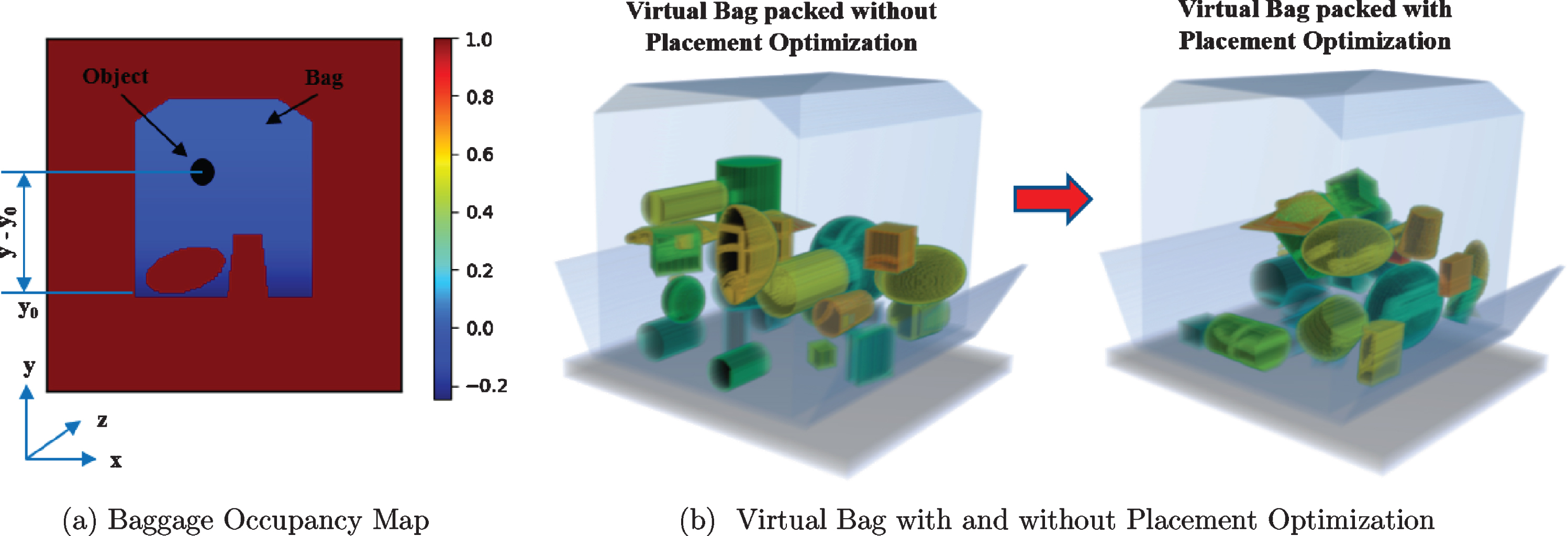
Object Placement Optimization: (a) Baggage occupancy map as defined in Equation 1 - the occupied space within the bag as well as the baggage exterior are assigned a high positive cost while the vacant space is given a graded negative cost depending on its distance from the bag’s base. (b) An example of virtual bag generated with and without placement optimization - the optimization step eliminates the case of ‘floating’ objects within the virtual bag.

4.1.2 Instantiating, placing and deforming the sheet objects

The random instantiation of a deformable sheet object in a bag starts out by DEBISim first creating a flat rectangular sheet at the top of the bag. Subsequently, the algorithm presented in this section allows the sheet to settle down in the bag as it deforms in order to conform to the shapes of the objects already in the bag. The instantiated sheet is subject to the following two steps:

Initially, while being treated as a flat rigid object, the sheet undergoes the same motions that are dictated by the two heuristics presented in the previous subsection – except for the very important difference that the no-overlap condition is only applied to the end-points of the sheet. This part of the motion of a freshly instantiated sheet is best visualized through the depiction in the first two images in Fig. 6. The linear structure shown in the first image settles to the position and orientation shown in the middle image on the basis of the no-overlap condition applied to just the end points.

Subsequently, the sheet is deformed in order to make it conform to the top-most points of the previously placed objects underneath. This is done through an algorithm that was adapted from our recursive midpoint displacement path-planning algorithm presented in [23]. This algorithm, presented in Algorithm 2, recursively calculates the midpoint of the sheet, checks whether the midpoint takes up any occupied voxel in the baggage volume, and, should there be an overlap with one of the previously placed objects, displaces the midpoint to the nearest free voxel. This imitates the way a sheet would physically stretch and settle in a bag that already has other objects in it. The pseudo-code shown in Algorithm 2 invokes our original RMPD algorithm whose pseudo-code is shown in Algorithm 3.

Algorithm 2 Deformable Sheet Placement Algorithm:

Places a sheet object O⁽ⁱ⁾ within a virtual bag. Unlike other object shapes in Algorithm 1, the parameter O⁽ⁱ⁾ . x holds all the curve points for the deformed sheet and is initialized with sheet endpoints x_heur obtained using heuristic packing rules as shown in Algorithm 1.

1. Initialize O⁽ⁱ⁾ . x with the sheet endpoints: O⁽ⁱ⁾ . x ⟵ x_heur

2. Calculate the midpoint of the vertices, C_mid ⟵ midpoint (O⁽ⁱ⁾ . x)

3. ifC_mid is occupied do

4. Change C_mid to nearest free voxel

5. end

6. Add the point C_mid to curve points, O⁽ⁱ⁾ . x

7. Calculate a simplex set S for O⁽ⁱ⁾ . x, S = {(C_i, C_j, C_k) |pointsi, j, kare

connected}

8. for each simplex, S_i ∈ Sdo

9. S_i ⟵ Midpoint _ Recursion _ Rule (S_i) // See Algorithm 3

10. Add S_i to O⁽ⁱ⁾ . x

11. end

Algorithm 3 Mid-point Recursion Rule: Midpoint _ Recursion _ Rule (C_pts)

Runs the Recursive Mid-point Placement algorithm for deformable sheets. It called recursively for deforming the sheets till no points collide with the occupied voxels in the bag.

1. ifC_pts are spaced less than a voxel apart do

2. returnC_pts // Stopping criterion for recursion

3. Calculate the midpoint of the vertices, C_mid ⟵ midpoint (C_pts)

4. ifC_mid is occupied do

5. Change C_mid to nearest free voxel

6. C_pts,1 ⟵ Midpoint _ Recursion _ Rule (( C_pts , C_mid , C_pts [1]))

7. C_pts,2 ⟵ Midpoint _ Recursion _ Rule (( C_pts [1] , C_mid , C_pts [2]))

8. C_pts,3 ⟵ Midpoint _ Recursion _ Rule (( C_pts [0] , C_mid , C_pts [2]))

9. Add the points C_pts,1 , C_pts,2 , C_pts,3 to curve points, C_pts

10. end

11. return C_pts

4.1.3 Generating liquid-filled containers

DEBISim can also instantiate virtual liquid-filled containers for placement in a bag. These are used in a dataset for the training and testing of machine learning algorithms for detecting liquid explosives. A container for a liquid is instantiated in exactly the same manner as a bulk object to which is applied the same placement logic as described in Section 4.1.1. After the container has acquired its final position and orientation, it is filled with liquid material upto a randomly chosen specified level. Specifying the liquid level after the final placement of the container eliminates the need for re-evaluating the liquid level inside the container through its various motions required by the placement logic.

DEBISim has a separate database of liquid materials which allows the user to specify the types of liquids to be filled into a container.

4.2 Virtual bag generation – the manual mode

Because the automatic mode in DEBISim randomly assigns material properties to the objects as they are being packed in a virtual bag, it has little control over the composition of the objects that one may want to see placed around a target item representing an explosive. In order to generate more complex test cases when simulating virtual bags, DEBISim thus also includes a manual mode that allows a user to create a virtual bag by manually arranging its contents. Such bags can then be added to the automatically generated bags for creating more challenging datasets for machine learning algorithms.

The manual mode is run with the help of a user-interactive GUI shown in Fig. 8. The main feature of this GUI is the user-interactive 3D graphics editor which enables the user to manually add, select, modify and place items within the virtual bag. The GUI also provides dedicated panels to change the properties of the selected object, adjust the reconstruction setup as well as change the scanner configuration for data generation. The prominent features of the User-Interactive GUI include:

Fig. 6

Deformable Sheet Generation: An 2D example representation of how deformable sheets are generated and placed in the virtual bag. The sheet (yellow line) is first initialized as a rectangular membrane as shown in Step 1 (Since this is a 2D illustration, the membrane is represented by a line). Step 2 shows how the endpoints of the sheet are placed with the packing heuristics as described in Section 4.1.1. The sheet is then deformed using Algorithm 2 thus assuming the final form in Step 3.

Fig. 7

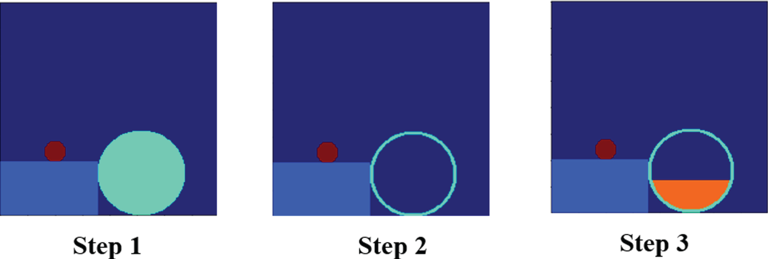
Generating Liquid Filled Containers: The example shows how a liquid-filled container is simulated in DEBISim. First, a container is instantiated and placed in the virtual bag in exactly the same manner as a bulk object. Once placed, the container is “filled” with the liquid up to a level chosen randomly.

Fig. 8

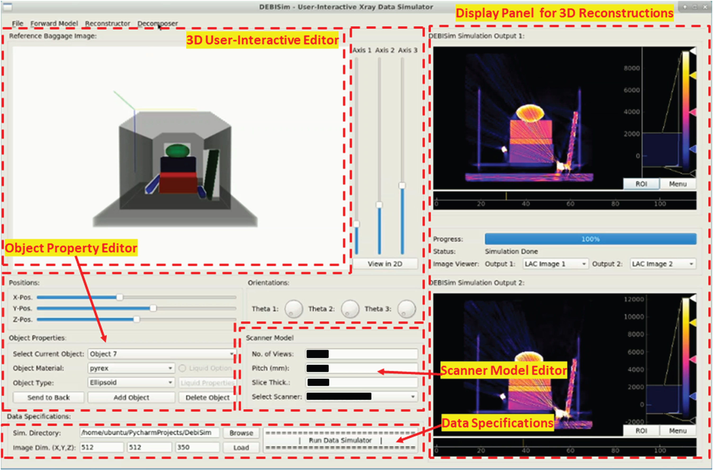
GUI for the Manual Mode for Generating a Virtual Bag: (a) The 3D User-Interactive Editor allows a user to manually pack a bag with different objects; (b) The Object Property Editor is for changing object properties such as scale, position, orientation, shape and material; (c) The Scanner Model Editor is for setting the scanner configuration; (d) The Data Specifications panel is for selecting the different attributes; (e) The Display Panel is for visualizing the 3D reconstructions. Further information regarding this GUI is available at [24]. The details for the scanner model have been masked for proprietary resaons.

Interactive Object Manipulation: The 3D graphics editor in the GUI allows the user to scale, rotate and place a selected object in the virtual bag. Besides, there are additional controls in the Object Property Editor shown in Fig. 8 which allow for precise manipulation and placement of the object within the bag.

Simulating and Adding New Materials: The selected object in the graphics editor can be assigned a material label manually using the Object Property Editor. DEBISim contains a database of ordinary day-to-day materials for the user to select from as well as a list of commonly known explosives and their plasticized variants [16]. Additionally, the GUI contains support to add new compounds and mixtures to the database.

Custom Shape Selection: By default, the options for assigning a shape to the selected object include rectanguloids, ellipsoids and cylinders. But custom complex shapes can also be loaded and placed within the bag in the same way as described in Section 4.1.1.

Editing Data and Scanner Specifications: The user-interactive GUI also contains controls for changing the input and output image dimensions, the resolution and size of the projection data as well as the units for the output reconstructions to be generated. Furthermore, the GUI provides additional consoles to edit the scanner configuration and the X-ray spectral properties.

A detailed description of the GUI and the various operations that can be performed with it can be found on the DEBISim reference webpage [24]. A tutorial video on using DEBISim in the manual mode can also be found at [25].

4.3 X-ray forward modelling block

The X-ray forward modeler in the simulator pipeline generates projection data for the 3D virtual bag created by the first block in the pipeline (see Fig. 1). The X-Ray Forward Modeling Block uses the knowledge of the cone-beam scanner geometry, the spectral properties of the X-ray sources and the X-ray transmission curves for the different materials in a virtual bag to calculate the projection data for the scanned volume.

The X-Ray Forward Modeling Block implements the following equation to model the transmission of X-ray photons along a given direction through a bag: $P = - ln \sum_{E = E_{l}}^{E_{h}} (D_{g}^{(E)} \cdot Poisson {S (E) \cdot exp [- \int μ (l, E) \cdot dl]} + N (0, σ_{c}^{2})) + ln \sum_{E = E_{l}}^{E_{h}} S (E)$ (5) The different terms in the above equation stand for:

The term ∫μ (l, E) · dl is the line integral along the path l traversed by X-ray photons with energy E. The line integral is calculated for the voxel-wise linear attenuation coefficient μ (l, E) assigned to different material labels in the bag using attenuation curves obtained from the XCOM Photon Cross Sections database [17].

S (E) denotes the photon energy distribution for the X-ray source defined for the keV range [E_l, E_h]. The normalized spectral distribution for an X-ray source, as provided by the user, is multiplied by the total photon count when then gives the photon energy distribution S (E). Varying the total photon count allows one to adjust the signal-to-noise ratios and the degree of possible photon-starvation artifacts (for bags packed with heavily attenuating materials).

The line-integrals are calculated for each energy level with Poisson sampling employed to add quantum noise. The notation Poisson {·} indicates this incorporation of the Poisson effects.

In order to model the shot noise in the detector, the forward modeler adds a Gaussian noise $N (0, σ_{c}^{2})$ term as shown.

The term $D_{g}^{(E)}$ represents the energy dependent detector gain response.

The term $ln \sum_{E = E_{l}}^{E_{h}} S (E)$ is for the flat-field correction.

Using the line integrals thus calculated, the forward modeler constructs 3D sinograms for a spiral cone-beam scanner geometry like the one shown in Fig. 9. The geometric model for a spiral cone-beam scanner is constructed with the help of the modeling libraries from ASTRA Toolbox [8]. The toolbox allows the tunable parameters depicted in Fig. 9 to be set in order for them to conform to an actual scanner in the field. In particular, the specifications related to the detector dimensions, detector panel spacing and scintillator gain can be tuned to match those found in one’s own scanner setup. Typically, the forward modelling block constructs a pair of sinograms for two different X-ray sources for dual energy data processing. However, one can run the DEBISim pipeline for multiple X-ray sources as long as their spectral distributions are provided.

Fig. 9

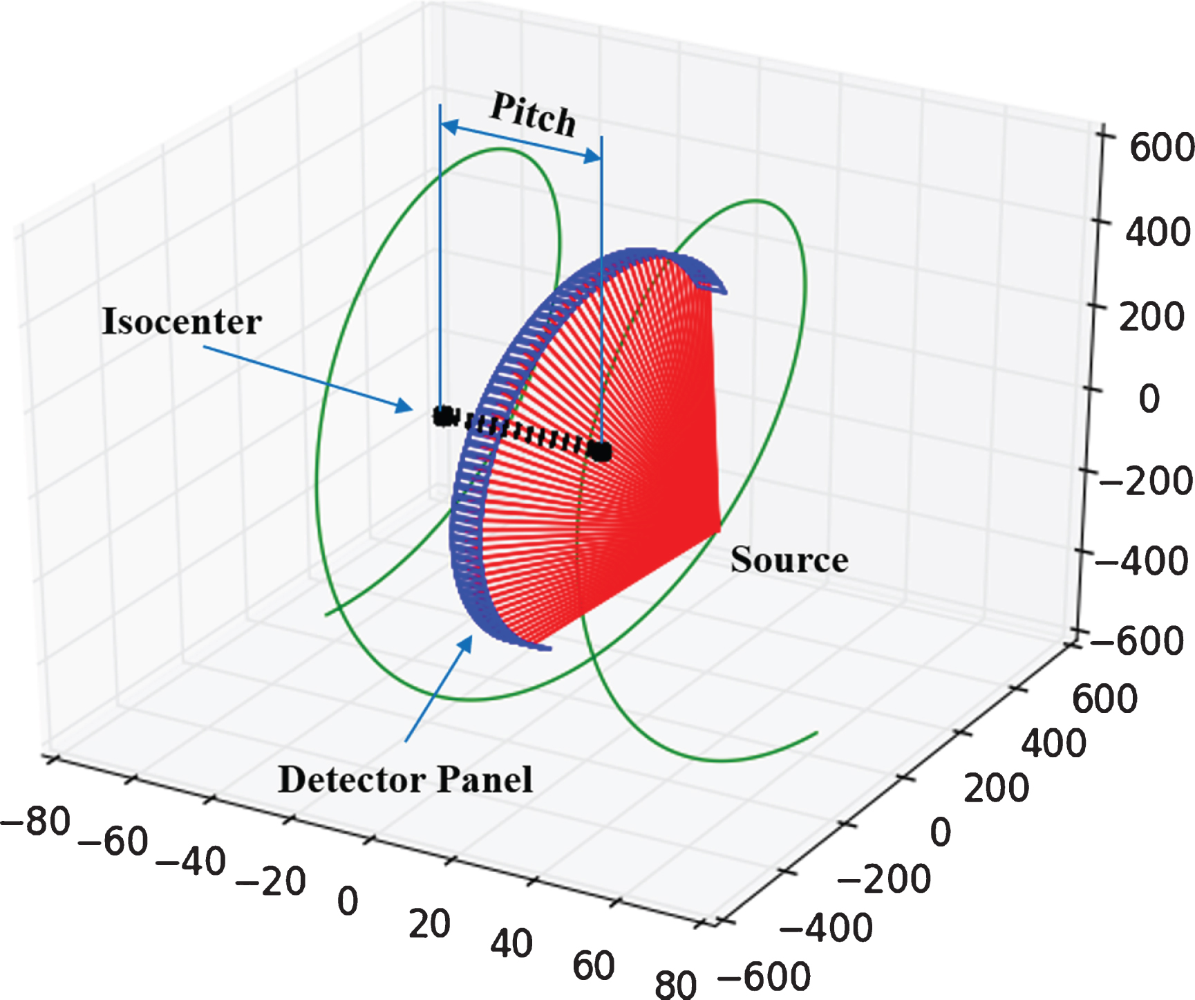
Spiral Cone-Beam Scanner Geometry: The spiral cone-beam scanner geometry used for simulation along with its geometric specifications.The scanner parameters shown in the diagram can be tuned by the user as per one’s own scanner setup.

4.4 Dual energy decomposition block

The Dual Energy Decomposition block processes the simulated X-ray sinogram pairs to extract additional material-based information from them. This is done by decomposing the dual energy projection data into Photoelectric-Compton coefficient line integrals using the dual energy models described in [2, 3]. The line integrals can be reconstructed and processed to obtain useful chemical properties like the effective atomic number and the electron density. The rest of this subsection presents a summary of how DEBISim carries out dual energy decomposition of the line integral data.

The starting point for dual-energy decomposition is a model that makes explicit the energy dependence of the X-ray attenuation μ (l, E) [2]. This energy dependence is expressed as a linear sum of two energy dependent basis functions, one representing the Compton effect and the other the Photoelectric effect: $μ (l, E) = a_{c} (l) \cdot f_{KN} (E) + a_{p} (l) \cdot f_{P} (E)$ (6) where a_p (l) and a_c (l) denote the PE and the Compton coefficients specific to the material at l ≡ (x, y, z) and where f_KN (E) and f_P (E) are the PE and Compton basis functions given by:

$\begin{matrix} f_{P} (E) & = & (1 / E)^{3} \\ f_{KN} (E) & = & \frac{1 + α}{α^{2}} [\frac{2 (1 + α)}{1 + 2 α} - \frac{1}{α} ln {1 + 2 α}] + \frac{1}{2 α} ln {1 + 2 α} - \frac{1 + 3 α}{(1 + 2 α)^{2}} \end{matrix}$ (7) with α = (E/510.975greaterthangreaterthanKeV). With this formulation, dual energy X-ray projections obtained for two different X-ray spectra S₁ (E) and S₂ (E) can be expressed as: $P_{1} = - ln [\int S_{1} (E) \cdot e^{{- A_{p} \cdot f_{p} (E) - A_{c} \cdot f_{KN} (E)}} \cdot dE] + S_{1, 0}$ (8) $P_{2} = - ln [\int S_{2} (E) \cdot e^{{- A_{p} \cdot f_{p} (E) - A_{c} \cdot f_{KN} (E)}} \cdot dE] + S_{2, 0}$ (9) where A_p = ∫a_p (l) · dl, A_c = ∫a_c (l) · dlgreaterthangreaterthan and where S_1,0 and S_2,0 represent flat-field correction. Here, A_p, greaterthanA_c, are the line integrals of the PE and Compton coefficients, a_p, a_c respectively. Since the spectral distributions for X-ray sources S₁ (E) and S₂ (E) can be determined beforehand, Eqs. (8) and (9) can be solved for measured projections $\bar{P_{1}}, \bar{P_{2}}$ as a nonlinear least squares optimization problem [3]: $A_{c}^{*}, A_{p}^{*} = \underset{A_{c}, A_{p}}{argmin} \sum_{i \in {1, 2}} [P_{i} (A_{c}, A_{p}) - \bar{P_{i}}]^{2}$ (10) The estimated photoelectric and Compton co-efficient integrals can be reconstructed and processed to obtain the two co-efficient images for material-specific properties like the effective atomic number [3, 5]. For example, the seminal work on DE decomposition [2] provides the formulation for the effective atomic number, Z_eff as a function of the Compton and the photoelectric co-efficients: $Z_{eff} = K {(\frac{a_{p}}{a_{c}})}^{1 / n}$ (11) where a_p, greaterthana_c are the voxel values obtained from reconstructed Compton and Photoelectric images and n, K are empirically determined constants. Some methods perform additional processing on the line integrals to estimate other parameters like electron density [4] or use other basis functions than f_p (E) , f_KN (E) to directly estimate the content of specific materials like water and iodine [26]. All these options for dual energy processing are available for the user to select from in the DEBISim pipeline. The end-product of this block is thus a set of co-efficient line integrals obtained from dual energy processing which are then reconstructed by the final pipeline block to get co-efficient images of the virtual bag.

4.5 Reconstructor block

The last block of the DEBISim pipeline shown in Fig. 1 reconstructs the co-efficient line integrals from the DE decomposition block to produce the CT attenuation images and the dual energy coefficient images. DEBISim performs spiral cone-beam CT reconstructions for the projection data using the weighted filtered back-projection (wFBP) method presented in [27, 28]. In the manual mode, the reconstructed images can also be viewed using the GUI in Fig. 8. For each simulated bag, the reconstructed images are also annotated with the ground truth material labels generated by the virtual bag generator.

Depending on the type of DE decomposition method used in the previous block of the pipeline, the reconstructed DE coefficient images can be further processed to obtain new coefficient images. For example, an effective atomic number (Z_eff) image can be obtained from the reconstructed Photoelectric and Compton images by using Equation 11. In case of the SIRZ and AdaSIRZ methods [4, 5], electron density and effective atomic number images can be calculated from the reconstructed SMB (synthetic monochromatic basis) co-efficient images.

5 Validation of the simulator

We have analyzed the simulation performance of DEBISim using a set of standard CT phantoms as well as different reference materials. The performance was evaluated on the basis of the accuracy of the reconstructed CT values and the fidelity in the reproduction of CT artifacts and noise. This section presents our validation experiments and their results. 2

5.1 Experimental setup

All experiments reported in this section were carried out on a cloud computing node with 24 VCPU cores, 32 GB RAM and a single GeForce Rtx2080Ti GPU. The scanner setup used for all the simulations reported here is that of a commercial dual energy spiral cone beam CT scanner used for airport security screening. 3 The setup uses a 160kVp X-ray source with filtration applied on alternating channels of rectangular detector panels to collect dual energy projection data. Unless otherwise specified, the baggage simulations were conducted for a scanned volume of dimensions 664greaterthanmm × 664greaterthanmm × 350greaterthanmm with a 1greaterthanmm³ voxel resolution. With regard to the time performance, with GPU support, it takes roughly 8 minutes to simulate the 3D projection of a virtual bag of the aforementioned dimensions and containing between 30 and 35 objects, with a total simulation time of about 20 minutes which covers the generation of the dual-energy sinogram pairs, dual-energy decomposition of the projection data and reconstruction of the single-energy and dual-energy CT images of the bag.

5.2 Tests with american college of radiology (ACR) phantom

The American College of Radiology (ACR) phantom [6] is a standard CT phantom used for assessing the performance of medical scanners. It consists of a cylindrical block made of water equivalent material divided into four modules, each used for testing different performance parameters. The real and the simulated reconstructions of the phantom are displayed in Fig. 10. We assess the accuracy of the reconstructed CT values of the simulation by using the first module of the phantom that contains four cylinders of different materials (bone, air, acrylic and polyethylene). The mean and the standard deviation of both the real and the simulated CT and Z_eff (obtained from dual energy data processing) values for these materials are compared in Table 1. We observe a high mean value accuracy for the simulation relative to the real CT scans while the standard deviation also falls within the same range.

Fig. 10

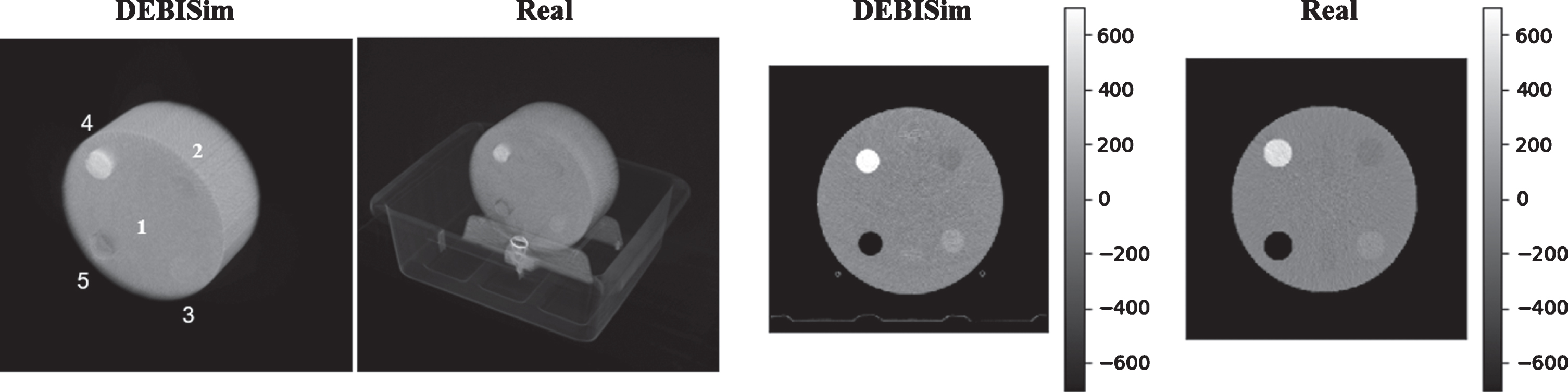
ACR Phantom Simulation: 2D and 3D illustrations of the simulated and the real scans for the ACR phantom [6] are shown in the figure. The different material labels are: (1) Water, (2) Polyethylene, (3) Acrylic, (4) Bone and (5) Air.

Table 1

ACR Phantom Simulation: Results for Material CT Value Accuracy

Label	Material	DEBISim		Real		Mean Value Ratio
		H^(S)* (MHU)	$Z_{eff}^{(S)}$	H^(R)* (MHU)	$Z_{eff}^{(S)}$	H^(S)/H^(R)	$Z_{eff}^{(S)} / Z_{eff}^{(R)}$
1	Water	1002 ± 38	7.60 ± 2.52	1016 ± 45	7.45 ± 1.88	0.98	1.02
2	Polyethylene	948 ± 23	5.54 ± 1.67	961 ± 38	6.09 ± 1.46	0.98	0.91
3	Acrylic	1085 ± 29	6.89 ± 2.02	1161 ± 41	8.91 ± 1.51	0.93	0.78
4	Bone	1513 ± 32	12.68 ± 1.7	1708 ± 43	12.90 ± 1.62	0.89	0.98
5	Air	20 ± 17	0	29 ± 29	0	0.69	N/A⁺

^* The CT Values are recorded in Modified Hounsfield Units, i.e., Hounsfield Units offset by 1000. ⁺ Vacant spaces containing only air are clipped during dual energy data processing to avoid noisy reconstructions.

5.3 Analysis using reference materials

Because the ACR phantom is primarily designed for medical scanning applications, the materials used in the phantom modules do not accurately represent the type of materials found in checked baggage scans. Hence, we have also tested the simulator using two additional sets of reference materials: the first set consists of low density materials (teflon, PVC, water, acetal and polyethylene), whereas the second set consists of high density materials (Al, Ti, Fe, Cu). These reference materials represent the range and type of materials that are frequently encountered in checked baggage. The comparison for the real and the simulated values is shown in Table 2. The reconstructions are shown in Figs. 11 and 12. The accuracy comparison between the simulated and the real scans in this experiment is along the same lines as in the previous experiment except for the highly attenuating materials such as copper.

Table 2
Analysis using Reference Materials

Label Material DEBISim Real Mean Value Ratio

H ^(S)* H ^(R)* H^(S)/H^(R)

Set 1 (Low Density)

1 Polyethylene 957 ± 5 1008 ± 21 0.95

2 Acetal 1341 ± 12 1423 ± 37 0.94

3 Water 1026 ± 50 1060 ± 14 0.96

4 Teflon 2124 ± 12 1991 ± 33 1.06

5 PVC 1456 ± 8 1655 ± 32 0.89

Set 2 (High Density)

1 Al 3166 ± 64 2946 ± 26 1.07

2 Ti 6753 ± 190 6387 ± 60 1.06

3 Fe 12661 ± 544 10516 ± 416 1.2

4 Cu⁺ 18808 ± 844 10593 ± 525 1.77

Label	Material	DEBISim	Real	Mean Value Ratio
Set 1 (Low Density)
1	Polyethylene	957 ± 5	1008 ± 21	0.95
2	Acetal	1341 ± 12	1423 ± 37	0.94
3	Water	1026 ± 50	1060 ± 14	0.96
4	Teflon	2124 ± 12	1991 ± 33	1.06
5	PVC	1456 ± 8	1655 ± 32	0.89
Set 2 (High Density)
1	Al	3166 ± 64	2946 ± 26	1.07
2	Ti	6753 ± 190	6387 ± 60	1.06
3	Fe	12661 ± 544	10516 ± 416	1.2
4	Cu⁺	18808 ± 844	10593 ± 525	1.77

^* The CT Values are recorded in Modified Hounsfield Units, i.e., Hounsfield Units offset by 1000. ⁺ A DC offset due to scattering effects is observed for heavy attenuating metals.

Fig. 11

Reference Materials- Set 1 (Low Density): 2D and 3D illustrations of the simulated and real scans for the reference materials are shown in the figure. The material labels are: 1 - Polyethylene, 2 - Acetal, 3 - Water, 4 - Teflon, 5 - PVC.

Fig. 12

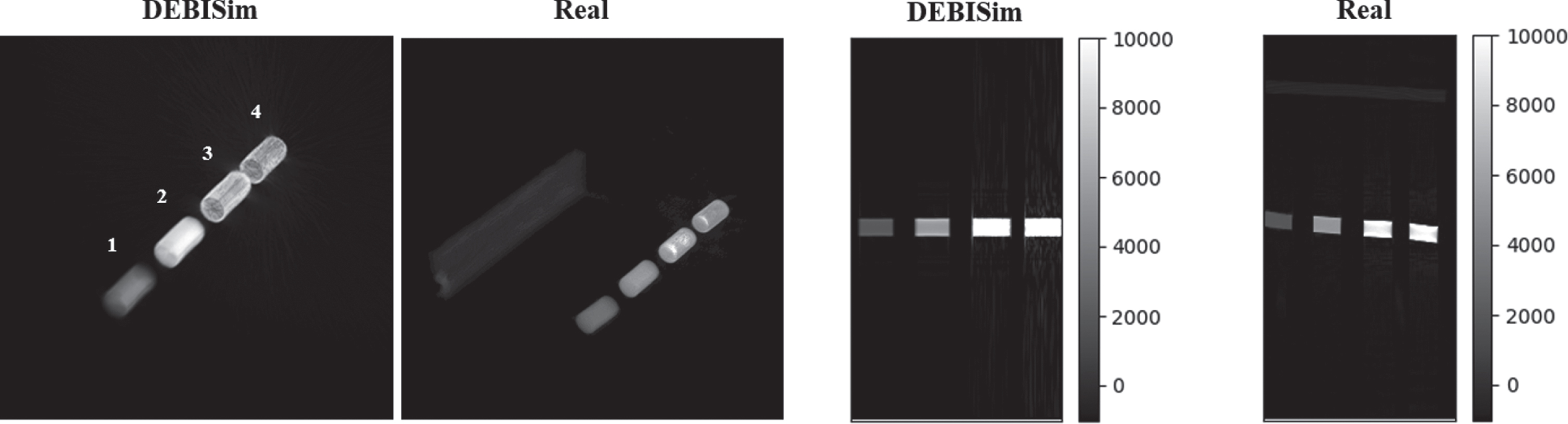
Reference Materials- Set 2 (High Density): 2D and 3D illustrations of the simulated and real scans for the reference materials are shown in the figure. The material labels are: 1 - Aluminum (Al), 2 - Titanium (Ti), 3 - Iron (Fe), 4 - Copper (Cu).

5.4 Tests with ANSI N42.45-2011 security screening phantoms

The ANSI Standard N42.45-2011 [7, 29] provides two CT phantoms for assessing the performance of X-ray security screeners. We have simulated both these phantoms using DEBISim for determining the quality of reproduction of CT artifacts and noise by the simulator. The two simulated phantoms are illustrated in Fig. 13. The different tests performed using the phantoms are as follows:

Fig. 13

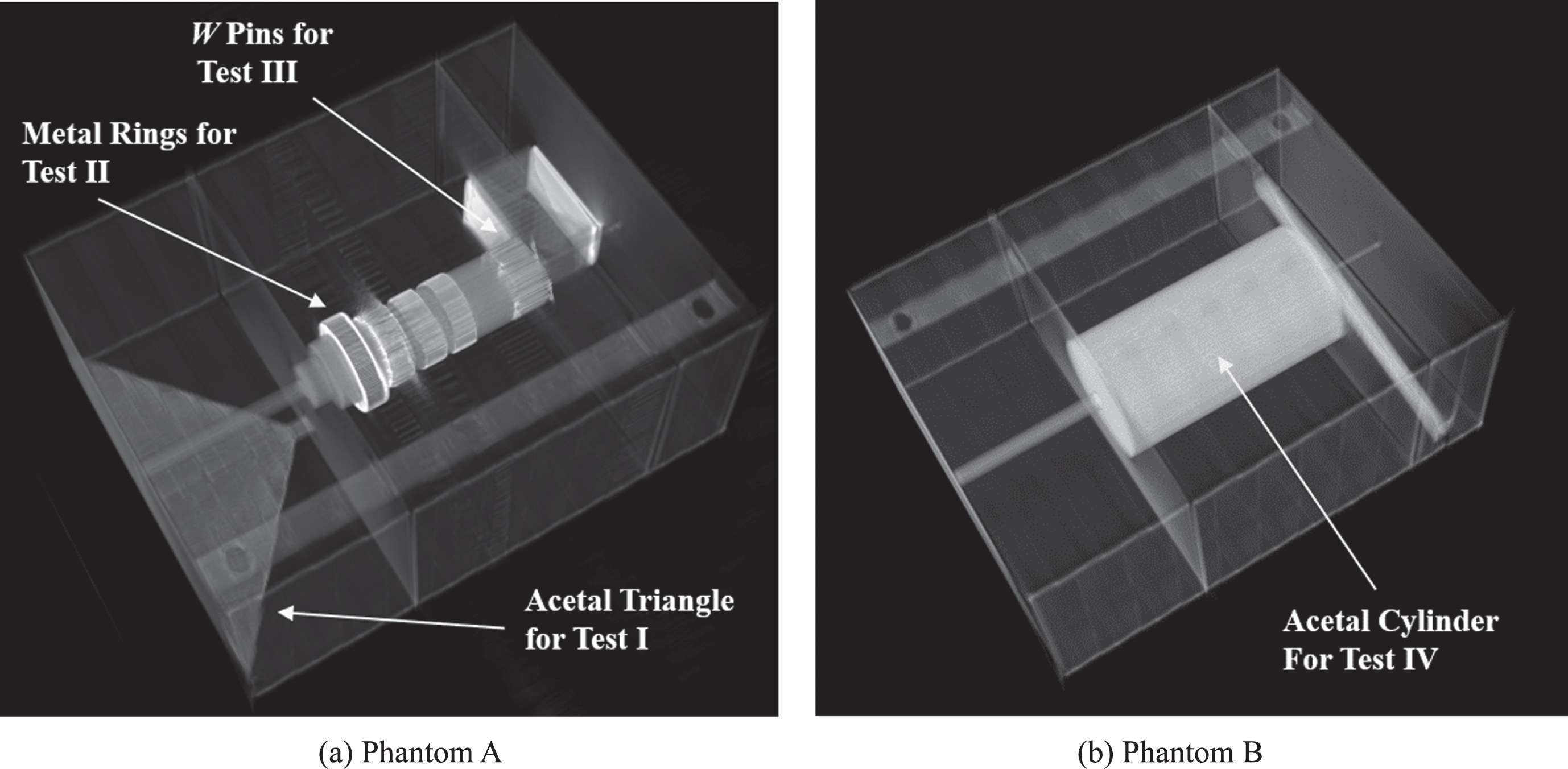
ANSI N42.45-2011 Security Screening Phantoms: The phantoms contain different “modules” for testing the simulations: (a) An acetal triangle for Test I (path length value drift); (ii) An acetal cylinder with metal rings for Test II (CT Value Uniformity); (iii) A cylinder with W pins for Test III (streaking effects); and (iv) A bulk cylinder for Test IV (CT statistics).

Test I – Comparing Photon Starvation Effects: An observable indicator of photon starvation in CT reconstructions is a drift in the median CT values for a homogeneous object with gradually increasing sizes of the cross-sections. The drift is caused by increased photon loss as X-rays traverse through longer paths in the larger cross-sectional parts in a phantom. The ANSI phantom A is used to measure this drift using an acetal triangular plate. The median CT value at points in the plate’s cross-section is measured along the helical axis and plotted against the cross-sectional length as shown in Fig. 14a. This drift in the CT values exists for both the simulated and the real CT reconstructions and the two are comparable.

Test II – Comparing Metal Artifact Effects: The central module within the ANSI Phantom A is an acetal cylinder fitted with four metal rings of increasingly attenuating materials. To test the effects of metal artifacts, we measure the mean and the variance of the CT values in the acetal cylinder cross-section that is surrounded by metal rings relative to the metal-free cross-sections of the cylinder. These values are plotted for the real and the simulated CT reconstructions in Fig. 14b. The plots show similar trends for the metal artifacts for both real and simulated scans. Note that the variance for the simulated scans is higher for the highly attenuating metals. This can be attributed to the higher order scattering effects in real scans becoming prominent for these metals. The plots that we see in the figure are obtained after adjusting the scintillator gain to account for these effects.

Test III – Comparing Streaking Artifacts: To study the streaking artifacts in the simulated scans, we use the second cylindrical module in NIST phantom A that contains four tungsten pins drilled into it. The intensity of the streaking artifacts is measured by the relative error in the CT values for the cross-sections between these pins. For the simulated scans, the relative errors in the CT value mean/standard deviation are found to be (11.0 % , ±34 %), which follows closely with the corresponding values for the real scan, (9.1 % , ±27 %).

Test IV – Comparing Bulk CT Value Statistics: The CT value distribution for the bulk acetal cylinder in NIST Phantom B is obtained for both the simulated and real scans giving a cross entropy score of 4.1 × 10^-1. It indicates that the two distributions for the CT reconstructions are similar.

Fig. 14

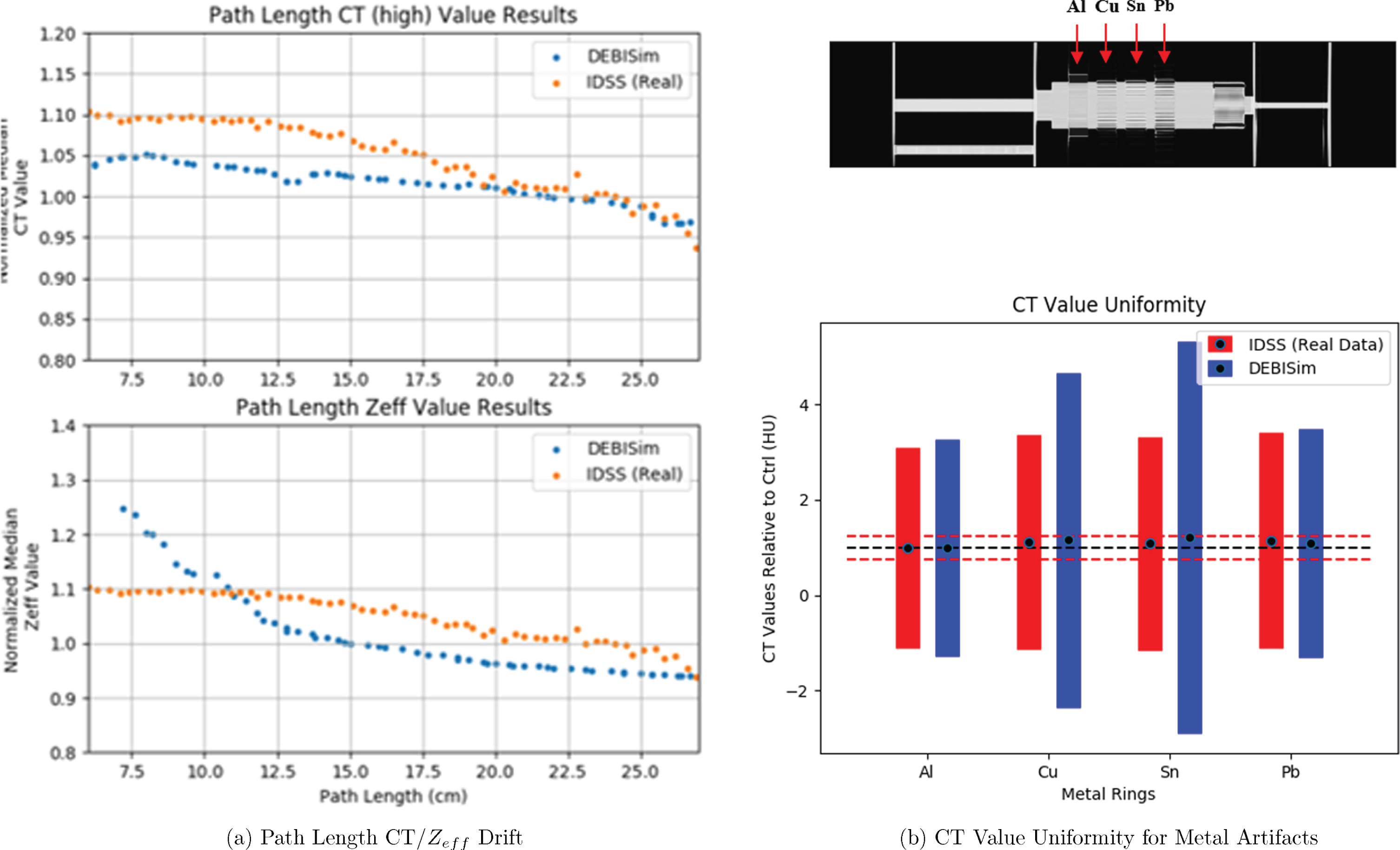
Test Results for ANSI N42.45-2011 Phantoms: (a) Path Length CT/Z_eff value drift test: Cross-sectional CT/Z_eff values are plotted for the acetal triangle against the length of the cross-section. The value drift denotes the degree of photon starvation in the scans. (b) CT value uniformity test: The error bars show relative deviation in the mean/standard deviation of acetal CT values in the presence of the metal rings. The red and black dashed lines show the reference acetal values while the blue and red errorbars shows the value spread for the real and the simulated scans for the different metal rings.

5.5 Examples of simulated baggage and baggage datasets

In this section, we describe and discuss examples of baggage samples and datasets that have been generated using the DEBISim pipeline. Figure 15 shows an example of a baggage data sample that is generated by DEBISim using the automatic mode described in Section 4.1. As shown in the figure, the simulator has instantiated a number of forms of objects within the virtual bag including deformable sheets, liquid-filled containers, and primitive shapes such as rectanguloids and a cylinder. In addition, the bag also includes complex objects such as mallets, bottles and cups whose 3D voxelized masks were obtained from the TO-4 objects database [18]. Figure 15 also shows the label image for the simulated bag with all the contents annotated by an integer label as well as the simulated CT and Z_eff reconstructions.

Fig. 15

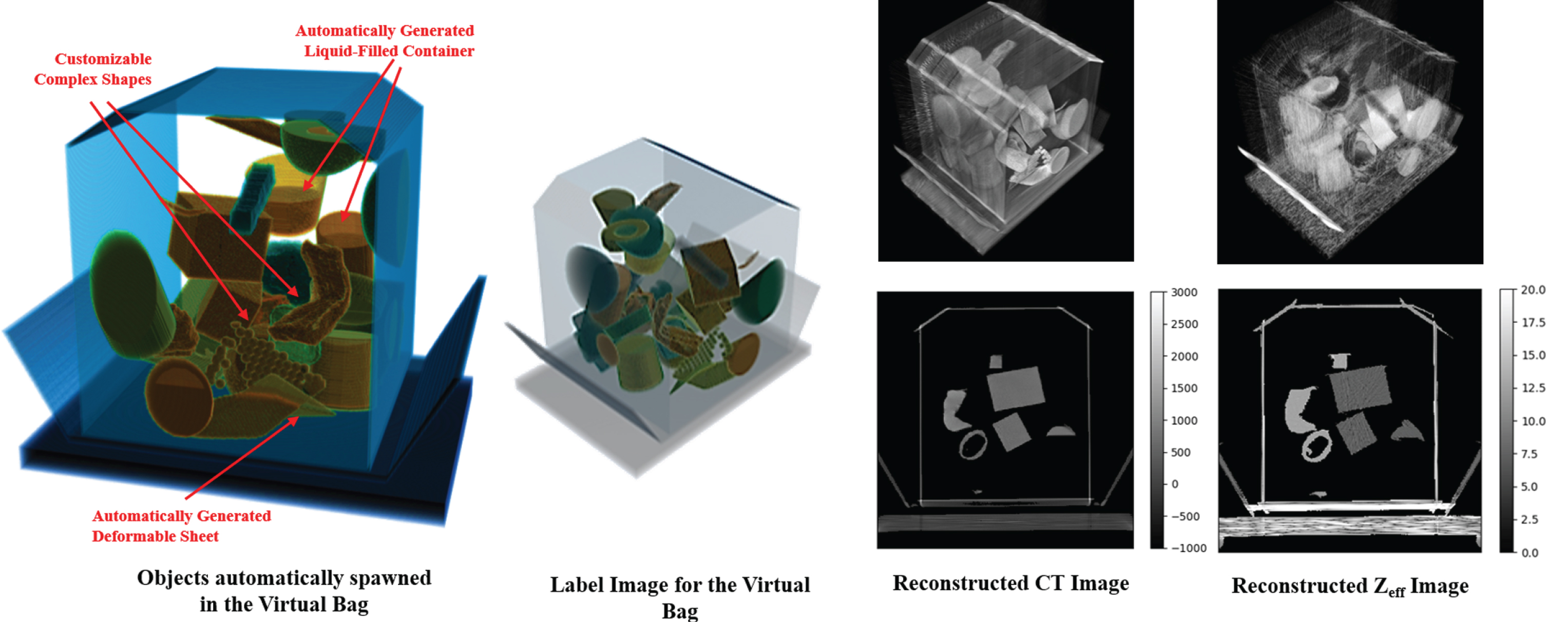
Baggage Simulation Example using DEBISim: The simulated bag consists of primitive shapes such as rectanguloids and cylinders, deformable sheets, liquid-filled containers as well as complex shapes such as mallets and bottles. The figure shows the label image for the simulation wherein every object in the virtual bag is annotated with an integer label. The simulated CT and Z_eff reconstructions are also shown.

Using DEBISim, we have created a number of different datasets for investigating different aspects of machine learning algorithms for automatic threat detection for bags. A list of generated DEBISim datasets can be found at the DEBISim reference webpage [24] and two of them have been described ahead.

Fig. 16 shows a few samples from the Complex Shapes Baggage dataset generated by DEBISim. The Complex Shapes Baggage Dataset contains 1200 simulated baggage samples with dual energy projection data generated for a spiral cone beam CT scanner. Each data sample in the dataset represents a virtual bag similar to the one shown in Fig. 15. The complex shapes used in this dataset were obtained from the TO-4 database [18]. The target threats generated in this dataset consist of rigid-body objects, deformable sheets as well as liquid threat items. The baggage samples are illustrated in Fig. 16 with two images, namely, the label image with each object annotated by an integer label as well as another label image showing all the target objects highlighted in red.

Fig. 16

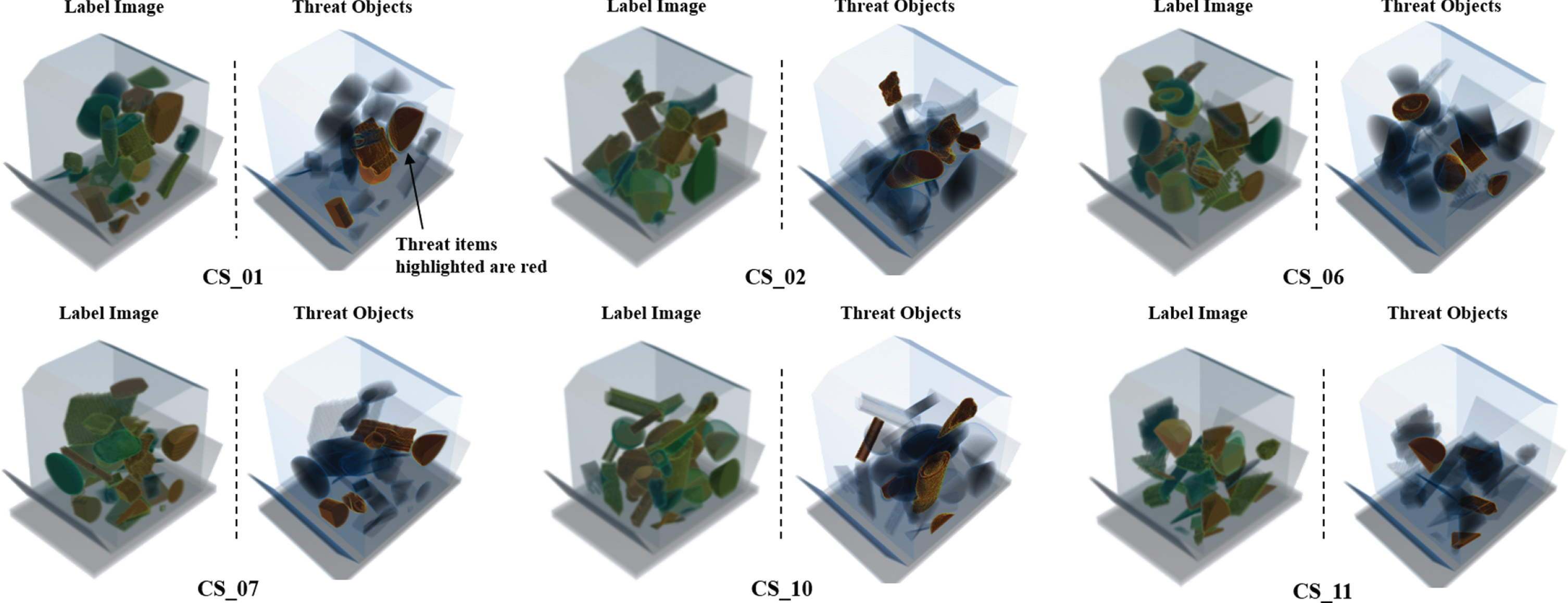
A subset of baggage samples from the Complex Shapes Baggage Dataset: For each illustrated baggage sample, the figure shows the label image for the simulation wherein every object in the virtual bag is annotated with an integer label and another label image with the target items highlighted in red.

Another dataset generated with DEBISim is the MAR Analysis Dataset shown in Fig. 17. Each of the 150 baggage samples in this dataset comprises of two sets of projection data, one with the bag containing all its contents intact, and the other with all the metal objects removed. Figure 17 illustrates a baggage sample from this dataset which also shows the difference in the CT reconstructions in the presence and absence of metals. The resultant reconstructed image pairs are useful in assessing the threat detection performance in presence and absence of metals.

Fig. 17

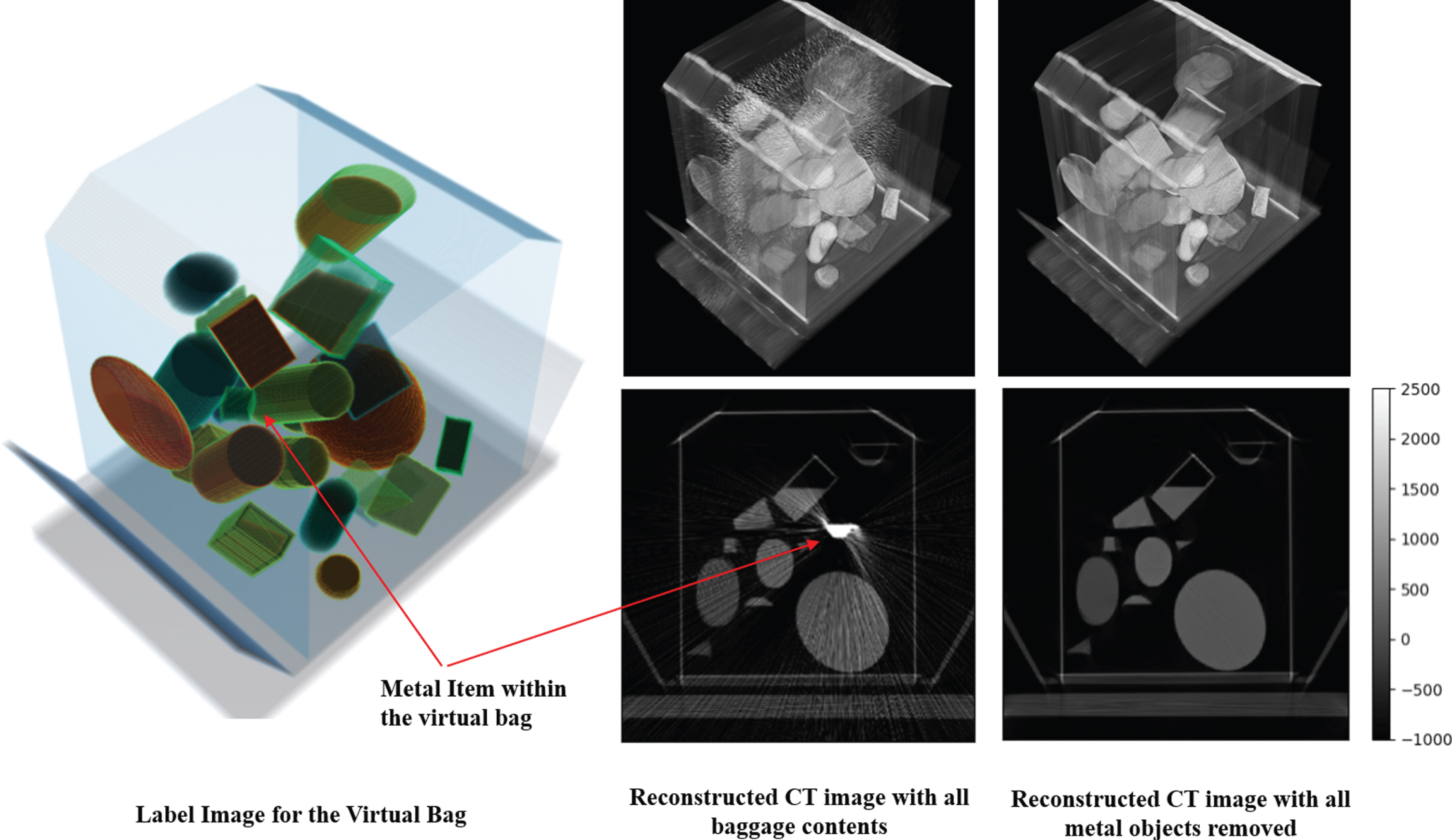
Data sample from the MAR Analysis Dataset: The MAR analysis Dataset uses the DEBISim pipeline to generate two pairs of simulated projection data for a virtual bag: (i) one with all the metal items intact and the other with all the metals items removed. The reconstructions for both pairs of data for the given example are also illustrated in the figure. This dataset is designed to assess the effect of metal artifact reduction on the performance of threat detectors.

6 Conclusion

This paper presented the DEBISim (Dual Energy Baggage Image Simulator) pipeline that lends itself well to the generation of large datasets needed for developing and testing modern machine learning algorithms for the automatic and semi-automatic detection of threats in checked and carry-on bags at the airports. DEBISim is an end-to-end simulator, in the sense that it is capable of (i) generating the bags with the user-specified diversity regarding the objects and the materials that are packed in the bags; (ii) generating the dual-energy projection data for the bags; (iii) carrying out dual-energy decomposition of the projection data for estimating the line integrals; and, finally, (iv) reconstructing the cross-sectional images for the desired parameters. While being an end-to-end simulator, DEBISim also allows its different blocks to be used independently.

Footnotes

A Particle swarm optimization

Particle Swarm optimization is a population-based global search strategy. It involves randomly spawning a set of candidate solutions or "particles" in the search space whose velocities are updated over iterations according to the local best position from the particle’s history and the global best position of the particle swarm. The update equations for a particle i in the PSO swarm at iteration k are given as: (12) $v_{k + 1, i} = w_{k} \cdot v_{k, i} + c_{1} \cdot r_{1} \cdot (x_{pbest, i} - x_{k, i}) + c_{2} \cdot r_{2} \cdot (x_{gbest} - x_{k, i})$ (13) $x_{k + 1, i} = x_{k, i} + v_{k, i}$ (14) $w_{k + 1} = w_{k} \cdot λ$ where x_pbest,i is the best position from the particle’s history, x_gbest is the globally best position in the current iteration, r₁, r₂ are the randomization variables and λ is the inertial factors. The social and cognitive weights c₁, c₂ along with λ are the hyperparameters for PSO optimization while the swarm size and number of iterations can also affect the PSO operation. An empirically accepted value set of λ = 0.5, c₁ = 4, c₂ = 4 is used for PSO in DEBISim. The number of particles is set to 100 and the optimizer is run for 200 iterations.

The simulation code along with its documentation and the examples presented in this section are available at the DEBISim reference webpage [].

The physical scans of the phantoms used and the specifications for this scanner were made available to us as a part of the BAA1703 AATR contract from the Department of Homeland Security. We are not at liberty to name the scanner model used or mention its spectral properties.

References

Wells

and Bradley

, A review of X-ray explosives detection techniques for checked baggage, Applied Radiation and Isotopes 70(8) (2012), 1729–1746.

Alvarez

R.E.

and Macovski

, Energy-selective reconstructions in x-ray computerised tomography, Physics in Medicine & Biology 21(5) (1976), 733.

Ying

, Naidu

and Crawford

C.R.

, Dual energy computed tomography for explosive detection, Journal of X-ray Science and Technology 14(4) (2006), 235–256.

Champley

K.M.

, Azevedo

S.G.

, Seetho

I.M.

, Glenn

S.M.

, McMichael

L.D.

, Smith

J.A.

, Kallman

J.S.

, Brown

W.D.

, Martz

H.E.

, Method to extract system-independentmaterial properties fromDual-EnergyX-ray CT, IEEE Transactions on Nuclear Science 66(3) (2019), 674–686.

Manerikar

, Li

and Kak

A.C.

, A spectrum-adaptive decomposition method for effective atomic number estimation using dual energy CT, Electronic Imaging 2020(14) (2020), 293–291.

McCollough

C.H.

, Bruesewitz

M.R.

, McNitt-Gray

M.F.

, Bush

, Ruckdeschel

, Payne

J.T.

, Brink

J.A.

and Zeman

R.K.

, The phantom portion of the American College of Radiology (ACR) computed tomography (CT) accreditation program: practical tips, artifact examples, and pitfalls to avoid, Medical Physics 31(9) (2004), 2423–2442.

Hudson

, Bateman

, Bergstrom

, Cerra

, Glover

, Minniti

, Seltzer

and Tosh

, Measurements and standards for bulk-explosives detection, Applied Radiation and Isotopes 70(7) (2012), 1037–1041.

van Aarle

, Palenstijn

W.J.

, Cant

, Janssens

, Bleichrodt

, Dabravolski

, De Beenhouwer

, Batenburg

K.J.

and Sijbers

, Fast and exible X-ray tomography using the ASTRA toolbox, Optics Express 24(22) (2016), 25129–25147.

Agostinelli

, Allison

, Amako

K.a.

, Apostolakis

, Araujo

, Arce

, Asai

, Axen

, Banerjee

, Barrand

, et al., GEANT4|a simulation toolkit, Nuclear instruments and methods in physics research section A: Accelerators, Spectrometers, Detectors and Associated Equipment 506(3) (2003), 250–303.

10.

Jia

, Yan

, Cerviño

, Folkerts

and Jiang

S.B.

, A GPU tool for effcient, accurate, and realistic simulation of cone beam CT projections, Medical Physics 39(12) (2012), 7368–7378.

11.

Browne

J.A.

, Mohan

, Martz

H.E.

Jr , Particle/Ray Interaction SimulationManager (PRISM) Assessment Report, Technical Report, Lawrence Livermore National Lab.(LLNL), Livermore, CA (United States), 2019.

12.

Llovet

, Fernández-Varea

, Sempau

and Salvat

, Monte Carlo simulation of Xray emission using the general-purpose code PENELOPE, Surface and Interface Analysis: An International Journal devoted to the development and application of techniques for the analysis of surfaces, interfaces and thin films 37(11) (2005), 1054–1058.

13.

Gong

, Stoian

R.-I.

, Coccarelli

D.S.

, Greenberg

J.A.

, Vera

and Gehm

M.E.

, Rapid simulation of X-ray transmission imaging for baggage inspection via GPU-based ray-tracing, Nuclear Instruments and Methods in Physics Research Section B: Beam Interactions with Materials and Atoms 415 (2018), 100–109.

14.

Coccarelli

, Hurlock

, Royse

, Carpenter

J.H.

, Greenberg

J.A.

, Johnson

, Bosch

, Gehm

M.E.

, Modeling real world system geometry and detector response within a highthroughput x-ray simulation framework, in: Anomaly Detection and Imaging with X-Rays (ADIX) IV, Vol. 10999, International Society for Optics and Photonics, 2019, pp. 1099906.

15.

Coccarelli

, Gehm

M.E.

, Greenberg

J.A.

, Modeling realistic virtual objects within a high-throughput x-ray simulation framework, in: Anomaly Detection and Imaging with X-Rays (ADIX) V, Vol. 11404, International Society for Optics and Photonics, 2020, pp. 1140402.

16.

Meyer

, Köhler

and Homburg

, Explosives, John Wiley & Sons, 2016.

17.

Berger

, Hubbell

, Seltzer

, Chang

, Coursey

, Sukumar

, Zucker

, Olsen

, XCOM: Photon Cross Sections Database, (version 1.5), [Online] Available: http://physics.nist.gov/xcom (Accessed 25th May, 2020).

18.

ALERT TO-4 ATR Initiative, 2014, “https://myfiles.neu.edu/groups/ALERT/strategic_studies/TO4_FinalReport.pdf”.

19.

Wang

, Megherbi

and Breckon

, A reference architecture for plausible Threat Image Projection (TIP) within 3D X-ray computed tomography volumes, Journal of X-ray Science and Technology 28(3) (2020), 507–526.

20.

Kennedy

and Eberhart

, Particle swarm optimization, in Proceedings of ICNN’95-International Conference on Neural Networks, IEEE 4 (1995), pp. 1942–1948.

21.

Press

W.H.

, Teukolsky

S.A.

, Flannery

B.P.

and Vetterling

W.T.

, Numerical recipes in For-tran 77: volume 1, volume 1 of Fortran numerical recipes: the art of scientific computing, Cambridge university press, 1992.

22.

Spong

M.W.

, Hutchinson

and Vidyasagar

, Robot modeling and control, John Wiley & Sons, 2020, pp. 113–148.

23.

, Manerikar

and Kak

, RMPD|A Recursive Mid-Point Displacement Algorithm for Path Planning, in: Proceedings of the International Conference on Automated Planning and Scheduling, Vol. 28, 2018.

24.

Manerikar

, Li

, Kak

, DEBISim - Dual Energy Baggage Image Simulator, 2020 (Accessed 21st January, 2020), https://engineering.purdue.edu/RVL/debisim/html/mainpage.html.

25.

Manerikar

, Li

, Kak

, DEBISim - Dual Energy Baggage Image Simulator, 2020 (Accessed 21st January, 2020), https://engineering.purdue.edu/RVL/debisim/html/attachments/debisim_video.mp4.

26.

Patino

, Prochowski

, Agrawal

M.D.

, Simeone

F.J.

, Gupta

, Hahn

P.F.

and Sahani

D.V.

, Material separation using dual-energy CT: current and emerging applications, Radiographics 36(4) (2016), 1087–1105.

27.

Stierstorfer

, Rauscher

, Boese

, Bruder

, Schaller

and Flohr

, Weighted FBP|a simple approximate 3D FBP algorithm for multislice spiral CT with good dose usage for arbitrary pitch, Phys in Med & Biology 49(11) (2004).

28.

Hoffman

, Young

, Noo

and McNitt-Gray

, FreeCT wFBP: A robust, efficient, open-source implementation of weighted _ltered backprojection for helical, fan-beam CT, Medical Physics 43(3) (2016), 1411–1420.

29.

IEEE-ANSI, N42.45-2011 - American National Standard for Evaluating the Image Quality of X-ray Computed Tomography (CT) Security-Screening Systems, ANSI Std. N42.45-2011 (2008).

30.

ALERT (Awareness and Localization of Explosive-Related Threats) Segmentation Initiative, 2013, https://myfiles.neu.edu/groups/ALERT/strategic_studies/TO3_FinalReport.pdf.

31.

Azevedo

S.G.

, Martz

H.E.

, Aufderheide

M.B.

, Brown

W.D.

, Champley

K.M.

, Kallman

J.S.

, Roberson

G.P.

, Schneberk

, Seetho

I.M.

and Smith

J.A.

, System-independent characterization of materials using dual-energy computed tomography, IEEE Transactions on Nuclear Science 63(1) (2016), 341–350.