Between-case standardized mean difference effect sizes for single-case designs: a primer and tutorial using the scdhlm web application

Abstract

Single-case research designs are critically important for understanding the effectiveness of interventions that target individuals with low incidence disabilities (e.g., physical disabilities, autism spectrum disorders). These designs comprise an important part of the evidence base in fields such as special education and school psychology, and can provide credible and persuasive evidence for guiding practice and policy decisions. In this paper we discuss the development and use of between-case standardized mean difference effect sizes for two popular single-case research designs (the treatment reversal design and the multiple baseline design), and discuss how they might be used in meta-analyses either with other single-case research designs or in conjunction with between-group research designs. Effect size computation is carried out using a user-friendly web application, scdhlm, powered by the free statistical program R; no knowledge of R programming is needed to use this web application.

Standardized mean difference effect sizes for single-case designs: a primer and tutorial using R

Single-case research designs (also referred to as “single subject designs”, “single-case experimental designs”, and “n-of-1 trials”; henceforth, SCRDs) have been used to assess intervention effects for many decades (Barlow & Hayes, 1979; Herson & Barlow, 1976). In contrast to experimental designs that involve comparing average outcomes across groups of individuals in different treatment conditions, SCRDs involve introducing an intervention to an individual case or cases and measuring changes in outcomes over time. Some types of SCRDs also involve removing and then re-introducing the intervention, providing further tests of the functional relationship between the intervention and the outcome. SCRDs are critically important for understanding the effectiveness of interventions for individuals with low incidence disabilities (e.g., physical disabilities, autism spectrum disorders), given the inherent difficulties in obtaining sufficient samples sizes for between-group experimental designs with such populations. As a result, SCRDs comprise a large part of the evidence base in certain areas within fields such as special education and school psychology. The results of SCRDs can under some circumstances provide a strong basis for understanding the causal effects of interventions (Gast & Ledford, 2014). They have the added advantage of providing information about intervention effects at the level of individual cases, whereas between-group experimental designs are informative only about average effects. Thus, the results of SCRDs are relevant for informing clinical and public policy decisions, and should be considered for inclusion in systematic reviews and meta-analyses that aim to synthesize the existing evidence about intervention effects (Council for Exceptional Children Working Group, 2014; Kratochwill et al., 2013).

However, inclusion of SCRDs in evidence reviews has been hindered by several related considerations. One consideration is that—due in part to tradition and in part to the statistical complexities introduced by hierarchical data structures and repeated measurement of outcomes—single-case researchers have historically relied on visual inspection of graphed outcome data to determine if an intervention has demonstrated an effect. While there have been efforts to develop systematic procedures for drawing conclusions using visual inspection, in practice the process can be subjective and ambiguous, and it can be difficult to train researchers to reach consistent conclusions from a common set of stimuli (Swoboda, Kratochwill, Horner, Levin, & Albin, 2012). Furthermore, visual inspection is usually focused on drawing conclusions about whether an intervention produces change in an outcome (i.e., the presence or absence of a functional relationship), rather than about the magnitude and consistency of those changes.

In our conversations with policy makers, the apparent subjectivity involved in analysis of single-case research troubles many potential users of this evidence—particularly those who are accustomed to using statistical estimation, confidence intervals, and hypothesis tests in an objective manner for drawing conclusions from between-group experimental studies. Although there has long been interest in applying the tools of systematic reviews and meta-analysis to data from SCRDs (e.g., Center, Skiba, & Casey, 1985; Gingerich, 1984; Scruggs, Mastropieri, & Casto, 1987), efforts to do so have until recently been hampered by a lack of well-grounded statistical methodology (Shadish, Rindskopf, & Hedges, 2008).

How things change. The past decade has seen growing interest in and rapid development of new methodologies for analyzing and synthesizing data from SCRDs (Shadish, 2014), as well as increased production of systematic reviews that incorporate or focus exclusively on SCRDs (Maggin, O'Keeffe, & Johnson, 2011). Innovations include new proposals for effect size metrics that quantify intervention effects for individual cases (see reviews by Manolov & Moeyaert, 2016; Parker, Vannest, & Davis, 2011); multi-level modeling approaches for synthesizing data from multiple SCRD studies (Moeyaert, Ferron, Beretvas, & Van den Noortgate, 2014; Van den Noortgate & Onghena, 2003, 2008); and frameworks for evaluating study quality (Wendt & Miller, 2012), including influential design and evidence standards proposed by the What Works Clearinghouse (Kratochwill et al., 2013) and the Council for Exceptional Children (Council for Exceptional Children Working Group, 2014).

Another recent advance has come with development of methods for translating findings from SCRDs in a way that makes them usable for meta-analysis alongside findings from between-groups studies. In particular, Hedges, Pustejovsky and Shadish (2012, 2013) introduced a statistical framework for estimating standardized mean difference effect sizes from SCRDs that are on the same scale as the standardized mean differences from between-group experimental designs. We refer to this effect size metric as the between-case standardized mean difference (BC-SMD) because it can be compared across the two types of study designs. Pustejovsky, Hedges, and Shadish (2014) extended the framework to handle more elaborate data generating models through restricted maximum likelihood estimation. BC-SMDs have been employed in meta-analyses that included both SCRDs and between-group designs (e.g., Losinski, Cuenca-Carlino, Zablocki, & Teagarden, 2014; Zelinsky & Shadish, 2016). Punja and colleagues (2016), for instance, considered the merits of combining evidence across the two types of designs.¹

Although researchers are beginning to apply BC-SMDs in meta-analyses of SCRDs, tools for computing these effect size estimates have not been readily available. The calculations entailed in obtaining an effect size estimate are not trivial, as they involve either nuanced algebraic formulas or iterative maximization techniques (i.e., restricted maximum likelihood estimation). Currently, the initially developed methods are implemented in an SPSS macro (Marso & Shadish, 2015), while the more flexible extensions based on restricted maximum likelihood (Pustejovsky et al., 2014) are only available in the form of a package for the R statistical computing environment (Pustejovsky, 2016).

The goal of this article is to illustrate how between-group standardized mean difference effect sizes, analogous to Cohen's d from a between-group randomized experiment, can be computed for two of the most widely used single-case designs: treatment reversal designs and multiple baseline designs. These effect sizes can then be weighted and synthesized in a meta-analysis that includes other single-case designs or even between-group designs. This article also provides a tutorial and demonstration of a free, user-friendly web application called scdhlm (short for single-case design hierarchical linear model) that can be used to compute these BC-SMD effect size estimates, including estimates from more elaborate and flexible models. The scdhlm web-app is powered by the R package of the same name, but includes a graphical user interface and thus does not require any knowledge of R.

In the sections that follow, we describe treatment reversal designs and multiple baseline designs and provide examples of these two types of single-case designs. We then discuss traditional case level effect sizes that have historically been used with single-case designs, followed by a discussion of the BC-SMD. The remainder of the article then provides a tutorial on how to use the scdhlm web application for estimating BC-SMDs.

Treatment reversal and multiple baseline designs

A hallmark of SCRDs is that outcome values for one or more participants are measured over multiple time points, with an intervention being introduced (and in some designs, withdrawn and reintroduced) at certain points in time for each individual participant. Different types of SCRDs use different strategies for monitoring and intervention. The treatment reversal design and the across-participant multiple baseline design are two of the most common SCRDs used in the literature (Shadish & Sullivan, 2011), and the two designs for which BC-SMD methodology currently exists. The remainder of this article therefore focuses exclusively on these two types of designs.

The treatment reversal design (sometimes called an ABAB design) involves a baseline phase (A) and an intervention phase (B), then reversal/withdrawal (A) and re-introduction (B) of the intervention; further repetitions of the withdrawal (A) and re-introduction (B) are sometimes implemented as well. In each phase of the design, the researcher collects measures of the dependent variable at multiple points in time and monitors the level and trend of the data series. Here, level refers to the average level of the outcome within a phase; trend (or slope) refers to change in the outcome across time-points within a phase. If a behavior changes upon introduction of the intervention and also upon withdrawal of the intervention, this is taken as evidence that the intervention has an effect (i.e., that there is a functional relationship between the intervention and the outcome). To improve the internal validity of the study design, it is recommended that the initial baseline phase (A) continue with repeated measurements until the outcome level and trend have both stabilized. Kratochwill and Levin (2010) describe several approaches to randomization in treatment reversal designs, which can also be used to bolster internal validity.

Treatment reversal designs are only appropriate when the intervention can feasibly and ethically be removed and when the effects of the intervention would be expected to dissipate after its removal (i.e., the outcome behavior of interest must be “reversible”). For example, if the intervention involves teaching a skill that is retained after acquisition, then a treatment reversal design would not be appropriate.² The What Works Clearinghouse SCRD standards indicate that a rigorous treatment reversal design should include at least four phases (thus providing three opportunities to demonstrate a functional relationship), each including five or more outcome measurements. Consequently, an A-B-A design that does not include a second intervention phase would not meet the WWC SCRD standards because it only provides two opportunities to test for a functional relationship.

Anglesea, Hoch, and Taylor (2008) used a treatment reversal design to test an intervention to reduce rapid eating among male teenagers with autism. The intervention involved giving the teens a pager that was set to vibrate at certain intervals (10 - 15 seconds, depending on the food), signaling that a reasonable amount of time had passed since the last bite of food. The study included three participants and four phases: an initial baseline phase (A), a pager phase (B), a withdrawal phase (A), and another pager phase (B). Each phase lasted between two and eight sessions (the mean number of sessions was slightly less than five per participant). There were two dependent variables: the total number of bites taken (which the intervention was not supposed to affect) and the number of seconds it took for the participant to finish his food (the target dependent variable). Visual inspection of the data from this study suggested that the intervention had its intended effect on the target dependent variable, in that participants took longer to eat when the pager was present than when the pager was not present (see Figure 1).

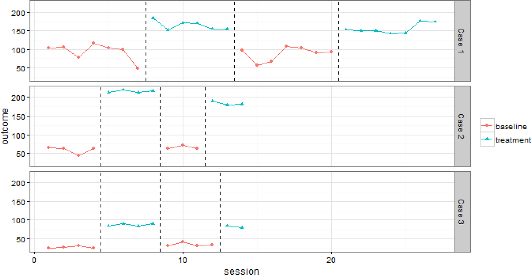
Example treatment reversal data from Anglesea et al. (2008)

In contrast to treatment reversal designs, multiple baseline designs involve systematically varying the timing of the introduction of the intervention across several cases, where a case may be either an individual, a setting, or a behavior. Multiple baseline designs can be conceived of as a series of stacked AB designs where the length of the baseline and intervention phases varies across cases. For example, in an across-participant multiple baseline, the first participant might have five observations during the baseline phase, with the intervention starting at the sixth observation; the second participant might have nine observations during the baseline phase, with the intervention starting at the tenth observation, and so on. Note that the order in which participants receive the intervention could be randomly determined, as could the intervention start times. Although randomization is relatively rare in practice, doing so does serve to increase the credibility of the results (Kratochwill & Levin, 2010).

For applying the BC-SMD effect sizes described in this paper, it will be important to distinguish between multiple baselines across participants, where cases correspond to different individuals, and multiple baselines across settings or behaviors, where a case typically corresponds to a common individual but measured in different settings or for distinct behaviors. BC-SMD effect sizes can only be calculated for across-participant multiple baseline designs for reasons explained in detail below.

An example of a study using a multiple baseline design is Laski, Charlop, and Schreibman's (1988) examination of a parent-training intervention designed to improve speech among children with autism. The study involved eight participating child-parent dyads, each of whom was measured under a baseline phase and an intervention phase. The intervention was implemented after the fourth, fifth, seventh, eighth, tenth, and eleventh baseline sessions. There were two dependent variables: parent verbalizations and child vocalizations. Visual inspection of the data from this study suggested that the intervention had its intended effect (see Figure 2 for child vocalization outcome data).

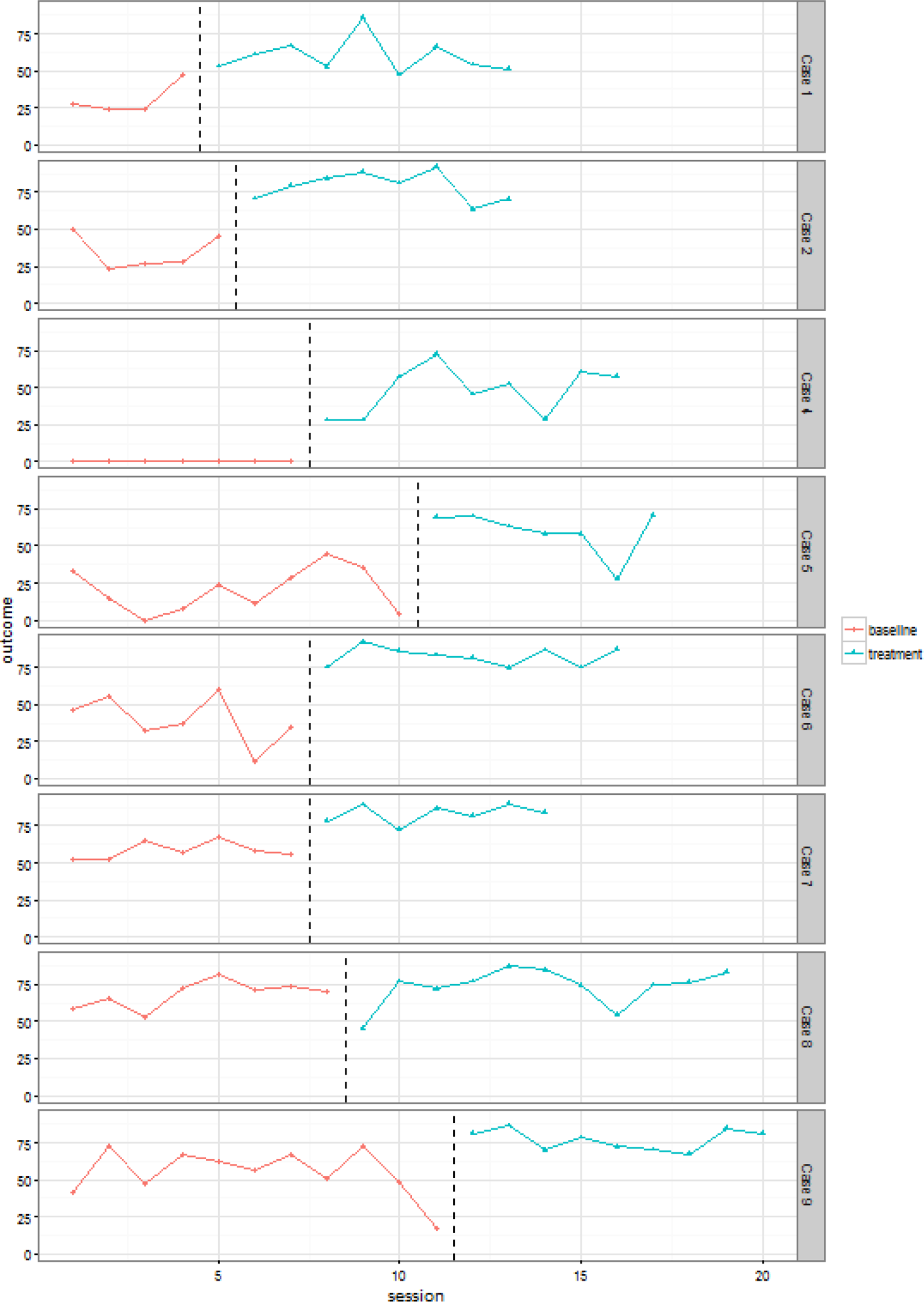
Example multiple baseline data from Laski et al. (1998)

Case-level effect sizes for SCRDs

Effect sizes are quantitative indices that characterize the magnitude and direction of some quantity of interest (in many cases, an intervention effect), and thus are useful for researchers, policymakers, and practitioners interested in the evidence base for an intervention; this assertion is true regardless of the type of research design being used. One important use of effect sizes is as inputs for quantitative synthesis or meta-analysis. A common problem in research synthesis is that a collection of studies to be synthesized might include primary studies that measure a common outcome construct, but use different operational definitions to do so. In such settings, it is critical to use standardized effect sizes, which capture the construct of interest but are not strongly influenced by procedural operations or sample size, and can thus be meaningfully synthesized to provide summaries of average effectiveness of an intervention across studies. Furthermore, effect size indices (whether standardized or not) need to have known sampling variances to be useful for conventional approaches to meta-analysis (Borenstein, 2009). A wide variety of effect size metrics have been proposed for use with SCRDs (for comprehensive reviews, see Parker, Vannest, & Davis, 2011; Pustejovsky & Ferron, 2016). Until recently, however, most effect size metrics available for SCRDs had undesirable properties that have made them unsuitable for inclusion in a meta-analysis.

The most common types of effect sizes that have been proposed for use with SCRDs are non-overlap indices, which all rely on examination of the distributional overlap of the outcome data across phases (Lenz, 2013; Parker, Vannest, & Davis, 2011). These include, for instance, the percentage of non-overlapping data (PND; Scruggs, Mastropieri, & Casto, 1987), the percentage of all non-overlapping data (PAND, Parker, Hagan-Burke, & Vannest, 2007), the non-overlap of all pairs (NAP, Parker & Vannest, 2009), and the percentage of data exceeding the median (PEM; Ma, 2006). Non-overlap indices are widely applied in systematic reviews of SCRDs (Maggin, O'Keeffe, & Johnson, 2011). However, these indices have also been criticized on methodological grounds. Shadish, Hedges, and Rindskopf (2008) note that these effect sizes have been developed without reference to parametric distributional modeling assumptions and thus lack known sampling variances. Consequently, these effect sizes cannot be synthesized with conventional meta-analytic techniques (which weight effect sizes by their sampling variances). Pustejovsky (2015) demonstrated that many of the non-overlap indices are strongly influenced by the procedural characteristics of a study's design, such as the number of observations in the baseline or treatment phases and the length of observation sessions used when measuring a behavioral outcome via systematic direction observation. Such sensitivities are undesirable because they make it difficult to compare the non-overlap indices across cases or studies that vary in procedural details, and thus reduce the suitability of the indices for purposes of meta-analysis.

Other standardized mean difference effect sizes have been proposed for use with SCRDs, which do have known sampling distributions (at least under certain modeling assumptions) and therefore can be synthesized using conventional meta-analytic techniques. For instance, Busk and Serlin (1992) proposed a standardized mean difference effect size, which is similar to the d-statistic used to quantify intervention effects in between-group designs except that their effect size is computed for each individual case and is standardized based on within-case variation. Specifically, the effect size is estimated as the difference in the mean of observations in the intervention and baseline phases, divided by the within-case standard deviation of the baseline observations. Other scholars have proposed variations of the standardized mean difference effect size that also account for trends and/or autocorrelation (Maggin et al., 2011; Van den Noortgate & Onghena, 2008), but all of these effect sizes are also standardized within-case. The logic of estimating effect sizes that are standardized within-case is consistent with the historical focus of most single-case research on visual examination and inspection of one case at a time. Indeed, as mentioned earlier, most SCRD researchers have not been historically interested in producing overall summaries of intervention effects across all cases, and thus these effect sizes standardized within-case have utility for their intended purpose. However, although effect sizes that are standardized within-case can be synthesized with each other in a meta-analysis, they cannot be combined in a meta-analysis that also includes standardized mean differences estimated from between-group designs. The problem is that effect sizes that are standardized within cases estimate a different parameter than that estimated by effect sizes that are standardized between cases (Shadish, Hedges, & Rindskopf, 2008; Van den Noortgate & Onghena, 2008).

Design-comparable effect sizes for SCRDs

In light of these issues, researchers may be interested in estimating effect sizes from SCRD studies that are comparable to those from between-group designs (i.e., standardized between-cases). Such design-comparable effect sizes could then be used to synthesize findings from both SCRDs and between-group designs in a single meta-analysis, or at least to make comparisons between findings from studies using each type of design. The standardized mean difference effect size statistics recently proposed by Hedges, Pustejovsky, and Shadish (2012, 2013) and extended by Pustejovsky, Hedges, and Shadish (2014) offer one promising family of design-comparable effect sizes that can be used with treatment reversal designs, across-participant multiple baseline designs, and across-participant multiple probe designs.

This effect size estimation approach involves modeling the data from treatment reversal and multiple baseline/multiple probe designs with a hierarchical linear model that accommodates the nested structure of SCRD data. Crucially, the hierarchical model captures variation in the outcome both within and across participants, making it possible to estimate a standardized mean difference effect size that is comparable to what would be obtained from a between-group design. However, because the BC-SMD effect size index involves across-participant variation in the outcome, it is only possible to apply the approach in designs that include multiple individuals. Consequently, the methods are not available for treatment reversal designs based on just a single individual, nor can they be applied in across-setting or across-behavior multiple baseline designs. In practice, the most basic versions of the BC-SMD estimation methods require that the study includes at least three individual cases, at minimum. Studies with more cases are ideal for increasing the precision of the effect size estimates and for calculating effect sizes based on more complex models.

The original estimators of these design-comparable effect sizes made several restrictive assumptions (e.g., baseline phases that are stable and lack trend; treatment effects that lead to a constant shift in mean levels; treatment effects that are homogeneous across cases). Thus, Pustejovsky and colleagues (2014) presented a more flexible modeling approach for estimating these design-comparable effect sizes, which uses a two-level formulation to model within-case (level 1) and between-case (level 2) means and variances. This more flexible modeling approach can incorporate time trends (homogeneous or variable across cases) and heterogeneous treatment effects across cases. In the remainder of this section, we describe the modeling assumptions behind this approach, beginning with the most basic version of the model.

Original model. The original estimators of BC-SMD effect sizes (presented in Hedges et al., 2012, 2013) are based on a certain hierarchical model for the data from a SCRD (cf. Shadish et al., 2014). This model makes several assumptions: 1.

the dependent variable was measured on a continuous scale that is common across cases;

the baseline phases are stable (lacking systematic time trends);

the intervention effect is an immediate change in the mean level of the outcome;

the intervention effect is homogeneous across cases;

the within-case errors and between-case variation are normally distributed; and

the within-case errors follow a first-order auto-regressive (i.e., AR(1)) process.

These assumptions can also be expressed as a hierarchical model for the data.

Suppose that the SCRD includes m cases, indexed by i = 1,…,m, and that case i is measured for a total of n_m measurement occasions, indexed by t = 1,…,n_m. Let Y_it denote the outcome from measurement occasion t for case i; let X_it be an indicator variable equal to 1 if case i was in the treatment condition during occasion t and equal to 0 if case i was in the baseline (or return to baseline) during occasion t. The individual-level model for the outcome measurements of case i is then

Y_{i t} = β_{0 i} + β_{1 i} X_{i t} + e_{i t}

where errors e_it are assumed to be normally distributed with mean zero and variance

σ^{2}

, and the errors for case i follow an AR(1) process such that

c o r r (e_{i s}, e_{i t}) = ϕ^{| s - t |}

for auto-correlation ϕ. Here, β _0i represents the baseline level of the outcome for case i, while β1_i represents the change in the level of the outcome upon introduction of the treatment (i.e., the individual-specific treatment effect). To complete the model, we must then make assumptions about how the individual-level model varies across cases. Specifically, the original model assumes that

\begin{array}{l} β_{0 i} = α_{0} + v_{i} \\ β_{1 i} = α_{1} \end{array}

where the between-case errors v_i are assumed to be normally distributed with mean zero and variance τ². Note that the individual-specific treatment effects are assumed to be equal across cases, so that α ₁ represents the common change in the level of the outcome upon introduction of the treatment. Note also that the within-case variance

σ^{2}

and auto-correlation ϕ are assumed to be constant across cases.

Under the assumptions of this hierarchical model, the BC-SMD effect size parameter is defined as

δ = \frac{α_{1}}{\sqrt{τ^{2} + σ^{2}}}

where the numerator α ₁ is the unstandardized effect of treatment and the denominator represents the standard deviation of the outcome, including both within- and between-case variation.

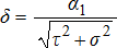
Originally, Hedges, Pustejovsky, and Shadish (2012, 2013) described methods for estimating the BC-SMD effect size δ based on moment estimation techniques. Later, Pustejovsky, Hedges, and Shadish (2014) introduced estimation methods based on restricted maximum likelihood (REML), which can also be applied under more general models. The original, moment estimation approach has the advantage that the estimates of the numerator and the denominator of the effect size will remain unbiased even if certain modeling assumptions do not hold. Specifically, the estimator of α ₁ will be unbiased even if the treatment effects are not exactly homogeneous across cases (assumption 4), while the estimator of the squared denominator,

τ^{2} + σ^{2}

, will be unbiased even when the errors are not normally distributed and do not follow an AR(1) process (assumptions 5 and 6). Modeling assumptions 4 through 6 only affect the small-sample correction used in the effect size estimate. In contrast, REML estimation might not have the same degree of robustness. However, when the modeling assumptions hold, Pustejovsky and colleagues (2014) found that REML estimation is somewhat more efficient than moment estimation, leading to more precise estimates of the BC-SMD. Furthermore, moment estimation techniques are only available for the original model, which makes other restrictive assumptions such as that the baselines are stable and treatment effects are immediate shifts in level, whereas REML estimation can be applied more generally.

More general models. Pustejovsky, Hedges, and Shadish (2014) described a general framework for estimating BC-SMDs under more general hierarchical models for SCRD data, focusing specifically on models for across-participant multiple baseline designs and using REML estimation. The basic hierarchical model can be extended in two main ways: by using a more flexible individual-level model and/or by making different assumptions about how the components of the individual-level model vary across cases. Here, we only sketch some of the possibilities, so interested readers may wish to refer to Pustejovsky, Hedges, and Shadish (2014) for further details.

We will first consider how to extend the individual-level model to handle time trends. With Y_it and X_it defined as previously, let T_it denote the time-point of measurement occasion t for case i and let Z_it denote the number of measurement occasions since the initial introduction of treatment for case i. As an initial example, we might assume that the outcomes for case i follow a linear time trend during the baseline phase and that introduction of the treatment leads to an initial change in level as well as a change in the slope of the time trend, as in:

Y_{i t} = β_{0 i} + β_{1 i} T_{i t} + β_{2 i} X_{i t} + β_{3 i} Z_{i t} + e_{i t},

where we again assume that the errors e_it are normally distributed with mean zero and variance σ², and that the errors for case i follow an AR(1) process with auto-correlation . More generally, we might assume that the baseline time trend is a p-degree polynomial, such as a quadratic (p = 2) or cubic (p = 3), and similarly that the treatment effect can be described by a q-degree polynomial. The individual-level model would then be:

Y_{i t} = β_{0 i} + β_{1 i} T_{i t} + … + β_{p i} T_{i t}^{p} + + β_{p + 1, i} X_{i t} + β_{p + 2, i} Z_{i t} + … + β_{p + 1 + q, 1} Z_{i t}^{q} + e_{i t},

where the terms β _0i, …, β _{p i} describe the individual-specific time trend during the baseline phase and the terms β _p+1,i, …, β_p+1+q,i describe the individual-specific pattern of change due to treatment. The scdhlm web application described in the next section allows the user to select up to a 6-degree polynomial for modeling each phase; however, we expect that much lower-order models, such as linear models, will usually be sufficient in practice.

Using a more flexible individual-level model requires making further assumptions about how the terms of such a model vary across cases within the SCRD. The original formulation of the model assumed that only the baseline levels of the outcome varied across cases, while constraining the treatment effects to be constant across cases. This restrictive assumption is not necessary with the more general formulation; one could instead allow the treatment effect to vary across cases. If the individual-level model includes time trends for the baseline or treatment phase, then one must also make assumptions about how the time trends vary across cases. In principle, we could allow all of the time trends to vary across cases. For example, in the model with linear time trends for each phase, we might assume that (β _0i, β _1i, β _2i, β_3i) follows a multivariate normal distribution with mean (0, 0, 0, 0) and a 4 × 4 variance-covariance matrix T. However, given the small number of cases available in most SCRDs, making more parsimonious assumptions will be necessary in practice. Pustejovsky, Hedges, and Shadish (2014) provided simulation evidence that effect size estimates from models with two random effects (e.g., baseline intercepts and baseline trends that vary across cases) have reasonably small biases when based on as few as four cases, even though REML estimation does not always converge with so few cases. Models with three or more random effects will likely require a larger number of cases.

When defining effect sizes under more general models, using these more flexible models for the data from SCRDs introduces additional complexities into the definition of the BC-SMD effect size. Recall that the BC-SMD parameter has two components: a numerator that represents the unstandardized treatment effect and a denominator representing the square root of the total variance in the outcome, including both within- and between-individual variation. However, in models that include polynomial time trends during the treatment phase, the unstandardized treatment effect is not constant across time points. Similarly, in models in which the time trends in either phase vary across cases, the total variation in the outcome is not constant across time points.

To operationally define a BC-SMD effect size index under models such as these, Pustejovsky and colleagues (2014) proposed that one specify a hypothetical between-group randomized experimental design. In this design, treatment is introduced to all cases starting at a certain point in time A (the initial treatment time), and outcomes are measured on all cases at a certain, later point in time B (the follow-up time). Given these hypothetical design parameters, the numerator of the BC-SMD is taken to be the effect of treatment at the specified follow-up time (i.e., after B – A + 1 sessions of treatment), whereas the denominator of the BC-SMD is taken to be the square root of the total variance in the outcome at the follow-up time. The BC-SMD effect size will depend to some degree on the user's choice of initial treatment time and follow-up time.³ The web application described in the next section allows the user to specify values for these quantities and examine the sensitivity of the results to varying choices.

Estimating design-comparable effect sizes using scdhlm

The design-comparable effect sizes for treatment reversal and multiple baseline designs originally developed by Hedges, Pustejovsky, and Shadish (2012, 2013) and extended with a more flexible modeling approach by Pustejovsky, Hedges, and Shadish (2014) can now be estimated using a free, user-friendly web application (or “app”) called scdhlm— short for single-case design hierarchical linear model. In this section, we describe how to use the app to calculate estimates of BC-SMD effect sizes for SCRDs. We begin by explaining how to access the app and load in data from a SCRD. We then explain the choices involved in selecting a model and obtaining a BC-SMD estimate in the context of two examples, including one from a treatment reversal design and one from an across-participant multiple baseline design.

Accessing the scdhlm app

The scdhlm app can be accessed in two ways. The simplest way to access it is via the web, at https://jepusto.shinyapps.io/scdhlm/ . This version of the app is hosted by a web service called shinyapps.io, which imposes limitations on the number of concurrent users of the site and total hours of active use of the site. Consequently, you might find that the site is not always available. If you intend to use the app extensively, we therefore encourage you to follow the steps below to install it on your own computer. Installing the app on your own computer and accessing the app in this manner has the further advantage that it will tend to run faster than it does over the web.

To run the app on your own computer, you will need to install two pieces of software (R and RStudio), both of which are open-source, freely available, and run on a variety of operating systems. After installing R and RStudio, you will then need to follow several additional steps to configure that software. Again, although this method of installation requires more time for setup than simply accessing the app on the web, it has the benefit of letting you run the simulator as much as you want, at faster speeds than over the web, and without Internet access. 1.

Install R from http://cran.r-project.org/ . Note that as of this writing, the app requires R version 3.0.1 or higher.

Install RStudio from http://www.rstudio.com/products/rstudio/download/ .

Once you have installed these programs, you will need to install several R packages. Do this by typing the following commands at the console prompt (you can also copy and paste the code into RStudio):

install.packages(“ggplot2”)

install.packages(“shiny”)

install.packages(“markdown”)

install.packages(“scdhlm”)

After all of these packages are installed, type the following commands at the console prompt to start the simulator:

library(scdhlm)

shine_scd()

The app should then open in your default web browser. Note that once the packages have been installed, these last two lines of code are all you will need to enter in order to launch the app.

To exit the simulator, close the browser tab in which it appears and click the red “Stop” icon in the upper right-hand corner of the RStudio console window.

Upon first accessing the app, you will be taken to the main page (tab), which provides basic information about the app, instructions for accessing the app, and references to the relevant journal articles on BC-SMD effect sizes. Note that the app version number and suggested citation for the software (Pustejovsky, 2016) are included on the ‘About' section of this home page.

Loading data

The app's Load tab allows you to load several example data files (for both treatment reversal and multiple baseline designs), or to upload your own data from an existing file. When uploading your own data file, it must be a text file that uses commas, semicolons, tabs, or spaces to separate entries. The file itself can have a .txt or a .csv extension. A spreadsheet is probably the most common and easiest way to enter and organize data, and most spreadsheet applications have the ability to save the data as either file type (.csv or .txt). For example, Microsoft's Excel can save a spreadsheet as a comma-delimited file (.csv) or a tab-delimited text file (.txt); Google Sheets can save a spreadsheet as a comma-delimited file; and most statistical software such as SPSS, Stata, and R can export data to comma-delimited files.

Format requirements. For both the treatment reversal design and the across-participant multiple baseline design, the app expects the following variables: (a) a case identifier, (b) a condition indicator (baseline and treatment are the most common ways these are labeled in the single-case literature), (c) the session number (e.g., measurement occasion, week, session), and (d) the dependent variable. The case identifier and condition indicator variables can be formatted as text or using numerical codes. For example, the case identifier could use names (e.g., John, Julia), or numbers (1, 2), or a combination (Case 1, Case 2). The session number and the dependent variable must be stored in numeric format in the data file.

Once the data file has been prepared, click on the Load tab. Under “What data do you want to use?” there are two options: one for using example studies, and one to upload your own data. To upload your own data, select the radio button next to “Upload your data from a file”; click “Choose File” and navigate to your data file; then click “Open”. The app then needs three pieces of information about the format of your data. First, you can let the app know if your data file contains headers in row 1 (i.e., text labels corresponding to the variable names). Including headers in row 1 is highly recommended. Second, you must let the app know how the columns of data are separated (commas, semicolons, tabs, spaces). Third, you must let the app know whether text fields in your dataset are included with no quotes (e.g., Week), single quotes (e.g., ‘Week’), or double quotes (e.g., “Week”). After providing these three pieces of information, you will then need to use the drop-down menus on the right-hand side of the app to specify which columns of the data correspond to which variables (see Figure 3 for screenshot). Finally, you will need to specify which value of the condition indicator variable corresponds to the baseline condition and which value corresponds to the treatment condition. The app will make guesses (based on which value appears first in the data file) but users should verify that these are correct.

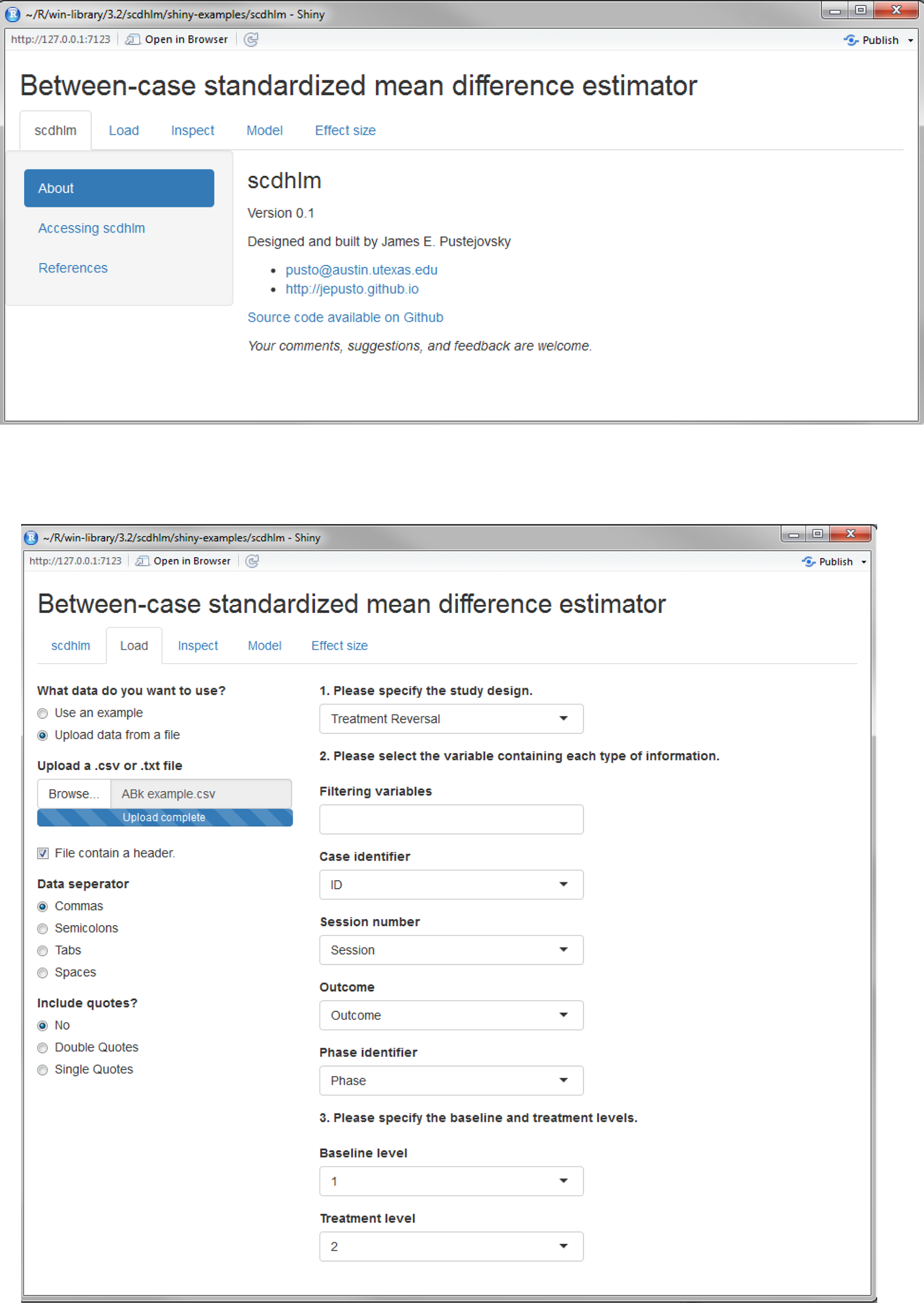
Screenshots of the scdhlm app

Inspecting loaded data. After loading your data into the app, click on the Inspect tab to verify that the data file was imported successfully and configured correctly. Selecting the Graph sub-tab will provide a graphical display of data for each case (similar to that shown in Figures 1-2). Selecting the Data sub-tab will display a table containing the data values for each case and measurement occasion.

Using the app with a treatment reversal design

In this section, we illustrate how to use scdhlm to calculate an effect size based on data from a treatment reversal design, available as one of the pre-loaded examples in the app. To follow along, click on the app's Load tab. Under “Choose an example”, click the dropdown box and select “Lambert (ABAB).” Then click the Inspect tab. Doing so brings up two tabs: one that displays the example data in graphical form, and one that shows the example data in tabular form.

This example comes from a study by Lambert, Cartledge, Heward, and Lo (2006), who examined a response card intervention designed to reduce disruptive classroom behaviors among fourth-graders. Students alternated between a single-student responding condition where teachers called on a single student to answer questions (A), and the response-card intervention condition where each student could respond to the teacher's question on a white laminated board (B). There were nine participants in the study (four in classroom A and five in classroom B), and four phases configured in an ABAB design. Each phase lasted between four and ten sessions. There were two dependent variables: disruptive behavior and academic responses; the example data file included with the app only includes the disruptive behavior outcome. Upon inspection of the loaded data, you can see each phase in the ABAB design clearly marked (A phases are shown in red, B phases are shown in blue). Visual inspection of the data for the first few participants also suggests that disruptive behavior tended to be lower in the intervention phases than during the baseline or return-to-baseline phases.

Model and estimation methods. The most difficult decision points when generating a design-comparable effect size are in the Model tab. The first consideration is which estimation method to use. The app currently supports two estimation methods: moment estimation and restricted maximum likelihood (REML) estimation, with REML as the default method. We recommend using REML in most cases because it is the most flexible estimation model. However, in certain situations moment estimation may be appropriate.

Moment estimation . The moment estimation method as originally proposed by Hedges, Pustejovsky, and Shadish (2012, 2013) offers the least flexible modeling approach for estimating design-comparable effect sizes. As noted previously, moment estimation is based on a data-generating model that makes several restrictive assumptions, including the assumptions that baselines are stable and lack trends and that treatment effects can be modeled by simple shifts in outcome levels. Thus, moment estimation is only appropriate to use in the absence of trends. On the other hand, when these assumptions are reasonable, moment estimation is robust to its other modeling assumptions, including normality and first-order auto-regression for the within-case errors—perhaps to a greater degree than REML. Our experience suggests that the assumptions behind the moment estimation approach are sometimes too restrictive, which is why REML is the default estimation method in the app.

Given the restrictive assumptions of the moment estimator, the app does not require any other model specifications under the Model tab for the moment estimator. After selecting the moment estimation approach, one can proceed to the final Effect size tab to view numerical results.

REML estimation . The REML estimation method offers a more flexible analytic model, and one that requires less stringent assumptions about the data-generating model. As such, we believe that REML estimation will be appropriate in most cases, particularly when treatment effects vary across cases or when there are trends in the baseline phase for multiple baseline designs (time trends are currently not available for treatment reversal designs).

If using REML as the estimation method, users will also need to specify whether the intercepts and/or treatment effects will be fixed or allowed to vary (i.e., include random effects). Models without time trends can include up to four components: fixed and random effects for the baseline level and fixed and random effects for the treatment level. The first two components are required in the app, while users can make choices about whether or not—or in exactly what form—to include the latter two components. Users who are unfamiliar with multilevel modeling (and the specification of fixed and random effects) may wish to refer to Shadish, Kyse, and Rindskopf (2013) for background on these models. 1.

Fixed effect for baseline level. Specifying a fixed effect for the baseline phase permits the intercept (level) across all baseline phases to be different from zero. The app currently requires that this fixed effect be included in the model, given that in most situations it will be unreasonable to assume that the average outcome value is zero across cases. Although there may be some situations in which it is reasonable to assume an average of zero in the baseline phase (e.g., when working with standardized scale scores, or scores that have been centered around zero), we expect that such situations will be relatively rare.

Random effect for baseline level. Specifying a random effect for the baseline phase level permits the intercept (level) across all baseline phases to vary across cases. The app currently requires that this random effect be included in the model, given that it is almost always appropriate to assume that the level of the outcome during the baseline phase will vary across cases. For instance, in the Lambert et al. (2006) example data, it is clear that the baseline phase levels vary across cases– ranging from around 7.5 in case A1 to 6 in cases B4 and B5. In situations where there is no variability in baseline phase levels (and thus the true random effects are actually zero), the model will simplify to only include the fixed effect.

Fixed effect for treatment level. Specifying a fixed effect for the treatment phase level permits the intercept (level) across all intervention phases to vary from the baseline phase level. The app requires that the treatment phase to have at least one term with a fixed effect. For treatment reversal designs, this term must be a change in level.

Random effect for treatment level. Specifying a random effect for the treatment phase level permits the treatment effect to vary across cases. To allow for randomly-varying treatment effects, click the check-box labeled “level” under “Include random effect” in the panel labeled “Treatment phase.” For modeling the data from Lambert et al. (2006), including a random effect for the treatment level leads to only a small difference in the resulting BC-SMD estimate. For sake of illustration, we therefore assume that the treatment effects are constant across cases by omitting the random effects for treatment phase level.

Displaying results. Once the model is specified, the app provides a graphical depiction of the fitted model for each participant. These graphs are the same as the graphs displayed in the Inspect tab, with the addition of a best-fit trend line for each phase. If using REML estimation, the trend lines represent Empirical Bayes estimates of the case-specific levels within each phase. If using moment estimation, the trend lines are maximum likelihood estimates of the case-specific levels within each phase. We recommend that users inspect the graphical output and fitted trend lines as a means of assessing model adequacy. In addition to the graphical output, the Model Estimates tab (next to the Graph tab) displays the raw statistical output from the fitted hierarchical model. Most users will not need to examine the output displayed in the Model Estimates tab. Advanced users may be interested in the output on this tab, as it provides the model specification and statistical output from R that underlies the estimation of the BC-SMD effect size and its standard error.

One important issue to note is that the fit statistics displayed at the top of the Model Estimates tab should not be used to compare the fit of different model specifications; these fit statistics are unstable when the design includes only a small number of cases, and thus usually should not be trusted. A second important issue to note is that the Model Estimates tab may also include an error message that the REML model did not converge, but users should not be concerned by this message. There is evidence from simulation studies (Pustejovsky et al., 2014) that indicates this REML estimation procedure can still yield close-to-unbiased estimates of the effect size parameter and its standard error even when the model does not converge.

Effect size estimation. The information most users will be looking for can be found in the final tab in the app, labeled Effect Size. Here, the effect size estimate and its standard error are displayed in the first two columns, and the lower and upper limits of a confidence interval are displayed in the next two columns. Users can specify the coverage level of the confidence interval using the input box provided, with the default set to 95%. The remaining columns describe the degrees of freedom, two nuisance parameters (the first order autocorrelation and the intraclass correlation; neither of which will be of interest to most users), and further information that is useful for archival and reporting purposes, such as the study design and estimation method. Users can click the “Download” button to create a comma-separated value file containing this summary output.

For the data from Lambert et al. (2006), using REML estimation without a random effect for treatment phase level yields a BC-SMD estimate of -2.40, with a standard error of 0.19 and a 95% CI of [-2.78, -2.04]. For this particular dataset, moment estimation yields quite similar results: a BC-SMD estimate of -2.51 with a standard error of 0.20 and a 95% CI of [-2.92, -2.13]. The close agreement between the two estimation methods provides some indication that the basic model applied here, which assumes a constant treatment effect, is a reasonable fit for these data. If there were larger discrepancies between the results based on the two estimation methods, this may indicate that some of the modeling assumptions are unreasonable.

Using the app with a multiple baseline design

The app provides several further options for modeling data from across-participant multiple baseline designs. To help users navigate these options, we now discuss another example, this time based on a multiple baseline design. To follow along, click on the app's Load tab, then click the dropdown box under “Choose an example” and select “Schutte (multiple baseline design).” Clicking the Inspect tab then allows the user to examine the data from this study in graphical or tabular form.

This example comes from a study by Schutte, Malouff, and Brown (2008), who examined the effects of a certain type of cognitive behavioral therapy on the fatigue severity of adults who suffered from prolonged fatigue. Thirteen participants were assessed during baseline phases that were two, five, or eight weeks long, after which they began intervention. Intervention phases lasted for up to seven weeks. Fatigue severity was assessed weekly using a self-report inventory.

Model and estimation methods. Users must make several choices about how to model the data from a multiple baseline design in order to generate a BC-SMD estimate. The Model tab lays out the available options. As with analysis of data from treatment reversal designs, the first consideration is whether to use moment estimation or REML estimation. Although moment estimation has some desirable robustness properties, it can only be applied in models that do not include time trends. Consequently, we focus here on REML estimation, which is also the default method.

REML: Phase time trends . If using REML estimation, users will need to select model specifications for the time trends in the baseline phase and in the treatment phase. The app can handle up to sixth degree polynomial trends for each phase, although we expect that most users will focus on a smaller set of just two possibilities: no trend (labeled as “level”) or linear trend. Statistical methods exist that can be used to determine the best-fitting type of time trend (i.e., likelihood ratio tests, model fit statistics). However, these methods may not work well in this context because they require a larger number of cases to function properly—more than are typically available from a SCRD. Our advice is to look at the data across participants within each phase to determine if the overall baseline level observed across participants seems to be unchanging (no trend), or increasing (or decreasing) in a linear fashion. Users should also be alert for different patterns, even knowing that they are likely to be rare. For example, a consistent U-shaped pattern across participants might indicate a quadratic trend.

By design, many SCRD studies will not exhibit baseline trends given that cases are sometimes dropped if they exhibit baseline trends and stability cannot be established.⁴ Trends in the treatment phase may be more common, however, given that not all treatments may have an instantaneous effect on the outcome. In general, when specifying the phase time trends used in the REML model for estimating design-comparable effect sizes, we recommend that users balance prior theory, visual inspection of the data, and parsimony. Parsimony is especially important, given that polynomial time trends have poor accuracy of extrapolation, particularly with short phases and/or a small number of cases. This is why we suggest that most users will probably focus on just the two simplest options of no trends or linear trends.

Another important consideration when specifying phase time trends is whether the user is estimating the design-comparable effect size to simply summarize the magnitude of the intervention effects for a single study, or is estimating the effect size for the purposes of including it in a synthesis (meta-analysis) with design-comparable effect sizes from one or more other studies. If the user is planning to include the effect size in a synthesis, we recommend that similar model specifications (i.e., phase time trends, and fixed/random effects, as described below) be used for all studies included in the synthesis.

For the example from Schutte, Malouff, and Brown (2008), we might reasonably assume no trends in the baseline and treatment phases. Visually inspecting the baseline data shown in the Inspect tab, it appears that most data points in the baseline phases are fairly stable. Similarly, although there are some fluctuations in outcomes in the treatment phase, there do not appear to be any consistently linear or quadratic patterns across cases. Thus, assuming no baseline or treatment phase time trends may be the most parsimonious assumption in this example.

REML: Fixed and random effects . If the user specifies time trends in either the baseline or treatment phase, they will also need to consider whether to include fixed and/or random effects for each of those time trends. The app will default to include fixed effects for each time trend, which will be reasonable in almost all situations. If the user assumes the baseline trends will vary across cases, then one may consider adding random effects to the baseline time trends. If the user also assumes that there are treatment-by-time interactions, adding random effects to the treatment time trends may also be appropriate.

As noted previously, when specifying the data-generating model underlying the design-comparable effect size, we encourage users to specify the most parsimonious model (in combination with expectations based on prior theory and visual inspection), and to select a model specification that will be appropriate to estimate effect sizes from all SCRD studies that will be included in the final meta-analysis (if a synthesis is planned). Furthermore, users should aim to specify the most parsimonious model possible, given that the small number of cases in most SCRD studies will prohibit reliable estimation of models with multiple random effects.

For the example from Schutte, Malouff, and Brown (2008), we might reasonably assume fixed and random effects at baseline, and fixed and random effects for the treatment phase level. Visually inspecting the baseline data shown in the Inspect tab, it is clear that the average baseline level is greater than zero and baseline levels vary across cases (e.g., in the 50-60 range for Case 8 versus 30-40 in Case 6). Further, visual inspection suggests that there is a change in level between the baseline and treatment phases, although this treatment effect varies across cases. Thus, allowing the baseline and treatment effects to vary across cases may be the more reasonable assumption in this example.

Multiple baseline designs - centering sessions. In models for multiple baseline designs that include time trends and that allow the time trends to vary across cases, the interpretation of the model estimates is contingent on how time is operationally defined. In particular, centering the time trend at a certain point changes the interpretation of the baseline intercepts, including both the fixed effect and the variance of the random effects, to correspond to the level of the outcome at the specified point in time (Singer & Willett, 2003). The app allows the user to choose the centering time point in order to provide a convenient interpretation of the model estimates. However, centering will not change the value of the effect size estimate displayed on the Effect size tab because BC-SMD is operationalized in way that is specific to a fixed length of treatment and a fixed point in time (see Pustejovsky et al., 2014 for more detail).

Testing hypotheses about treatment effects. A statistical test of the null hypothesis that the population average effect size is zero can be obtained on the Model tab. For example, for the Schutte, Malouff, and Brown (2008) multiple baseline study, and using the model specification outlined above (no time trends, fixed and random effects for level at baseline, and fixed and random effects for level in the treatment phase), the following output is generated:

Fixed effects: list (fixed)
	Value	Std.Error	DF	t-value	p-value
(Intercept)	49.05833	2.212868	131	22.169575	0.0000
trt	-3.17977	1.865172	131	-1.704815	0.0906

The p-value for “trt” (treatment) is .0906; this is the p-value for the statistical test associated with the population average treatment effect. Note that the output is configured to display p-values to four decimal places. If the output reads 0 or .0000, it should be understood (and reported as) p < .0001.

Effect size estimation. Compared to treatment reversal designs, the wider range of available options for modeling across-participant multiple baseline designs leads to further considerations for estimating BC-SMD effect sizes. In particular, in models for data from multiple baseline designs that include time trends, the user will need to specify two hypothetical experimental parameters on the Effect Size tab: the initial treatment time (A), and follow-up time (B). These values affect the numerator and denominator of the BC-SMD effect size, as described previously (also see Pustejovsky et al., 2014 for further details).

By default, the app chooses these times based on the phase lengths of the case that is first to enter treatment. Specifically, the default is to set the initial treatment time equal to the last measurement occasion before the first case enters treatment (i.e., the length of the shortest baseline phase) and the follow-up time equal to the initial treatment time plus the length of the treatment phase for the first case to enter treatment. Under most circumstances, we would expect that the default choice for the initial treatment time will be reasonable. However, users calculating BC-SMD effect size estimates for purposes of synthesizing multiple studies should consider choosing a common length of treatment (i.e., using a fixed value for the difference between the follow-up time and the initial treatment time) so that the resulting effect size estimates are based on a common operational definition. For the multiple baseline design conducted by Schutte, Malouff, and Brown (2008), the app defaults to use week 2 as the initial treatment time and week 9 as the follow-up time, for a treatment length of 7 weeks. These choices seem reasonable for this example because the treatment phase lasted 7 weeks for all but two of the cases.

It should be emphasized that users’ choices for these hypothetical experimental parameters do have consequences for the BC-SMD effect size estimates. The magnitude of the estimates will depend more strongly on the length of treatment (B – A) when the treatment phase exhibits steeper linear or polynomial time trends. The magnitude of the treatment effect estimates will depend on the choice of follow-up time if the model includes baseline time trends (either linear or polynomial) that vary across cases, with larger between-case variation leading to greater sensitivity.

For the example data from Schutte, Malouff, and Brown (2008), using the model specifications outlined above and the default initial treatment time and follow-up time leads to a BC-SMD estimate of -0.3125 (95% CI [-0.6997, 0.0615]). This estimate is not sensitive to the choice of hypothetical experimental parameters because we have assumed a model without time trends in either phase.

Using the design-comparable effect size in meta-analysis

Using the design-comparable effect size estimated with the scdhlm app in a meta-analysis is straightforward. Inverse variance weighting is the most common weighting scheme in meta-analysis (using fixed or random effects inverse variance weights). The scdhlm app reports the estimated effect size's standard error; squaring this value yields the effect size's variance. Taking the inverse of the variance yields a weight that could be used in a meta-analysis, assuming a fixed effect meta-analysis model (random effects models would additionally require inclusion of the between-studies variance in the denominator of the weight). For example, the effect size estimated for the Lambert et al. (2006) study, using the specifications outlined previously, has a standard error of 0.1906, therefore the variance is 0.1906², or 0.03632. The inverse of this variance is 27.53, which is the study's fixed effect weight that could be used in an inverse-variance weighted meta-analysis.

This suggests an important lesson. In a typical between-groups study that uses a post-test only analysis (e.g., an independent groups t-test) and the standardized mean difference (d) statistic as the effect size measure, the study's inverse variance weight is approximately one quarter of the total sample size. This value will vary somewhat depending on how close the group-specific sample sizes are to one another and on the observed value of d, but it is a reasonable rule of thumb. As such, the Lambert et al. (2006) study has approximately the weight of a between-groups study with about 100 participants. The typical sample size in studies reviewed by the U.S. Department of Education's What Works Clearinghouse is about 100 (Valentine, Wilson, Rindskopf, Lau, Tanner-Smith, Yeide, LaSota, & Foster, 2016). Therefore, the Lambert et al. study has about the same amount of information as a typically-sized study in education despite having only 9 participants. The reason for this is that the BC-SMD estimate makes use of the relatively large number of observations per phase in the ABAB treatment reversal design. We should note that the Lambert et al. study is relatively large for a single-case design study. Most SCRD studies will not have weights this large and will therefore contribute less to the overall mean effect size estimate in a meta-analysis. For example, the BC-SMD estimate from Anglesea, Hoch, and Taylor (2008) has a standard error is 0.9877. Squaring and inverting that statistic yields a weight of 1.03 (approximately equivalent to a between-groups design study with just four participants).

After computing a weight for each study, meta-analysis proceeds normally. Because the effect sizes we computed for SCRDs are comparable to standardized mean differences from between-group studies, they can in principle be included in a meta-analysis that includes both types of study designs. Zelinsky and Shadish (2016) provide a detailed demonstration of how to carry out such a meta-analysis. If appropriate, random effects weights can be computed in the usual manner (i.e., estimating the between studies variance component and adding that to each study's variance estimate, then computing the inverse of that value to find the random effects weight; see Hedges & Vevea, 1998). Pustejovsky, Hedges, and Shadish (2014) also recommend using robust variance estimation procedures (Hedges, Tipton, & Johnson, 2010) for meta-analysis of BC-SMD effect sizes, due to the possibility that the standard errors of the effect size estimates may be understated when based on a very small number of cases.

Conclusion

In this paper we discussed the development and use of effect sizes for two popular single-case research designs—the treatment reversal design and the across-participant multiple baseline design—and showed how they can be used in meta-analyses either with other single-case research designs or in conjunction with between-group research designs. We discussed how to carry out effect size computation with a user-friendly graphical user interface that sits on top of the statistical program R, and that does not require any background knowledge of R. Our hope is that we have provided sufficient guidance for readers to navigate the basic functionality available in the app and to start calculating effect size estimates for SCRD studies of interest.

The effect sizes we discuss in this paper involve characterizing average effects across multiple individuals, whereas many SCD researchers will also be interested in variation in individual-specific effects across participants in a study. This is an inherent limitation of the method—necessary for achieving design-comparability—because between-group designs provide information about average effects, rather than individual-specific effects. That said, this concern is analogous to moderation in between-group designs (e.g., the magnitude and/or direction of the treatment effect depends on some grouping variable), and future research might be able to bridge these two perspectives.

Future research should also investigate methods for model selection and model fit evaluation that work well with the data situations common in SCRDs (repeated measures on a relatively small number of participants). One approach might be to use statistical and visual analysis approaches together to help minimize the weaknesses of these approaches when used in isolation. Furthermore, it will be helpful for researchers to extend the design-comparability work, which to date has focused on the standardized mean difference effect size, to other families of effect sizes (such as odds ratios and response ratios) that are more appropriate for outcome data in the form of proportions (e.g., percentages of class time with a disruptive episode) or counts (e.g., number of outbursts during math class). Much interesting work remains, but we are hopeful that the progress made so far is helpful as researchers look to integrate evidence from SCRDs in order to better guide evidence-based practice and policy decisions.

Acknowledgement

Financial support from the American Institutes for Research for the production of this paper is gratefully acknowledged.

Footnotes

1

In general, we believe that the usual considerations about whether a particular study should be included in a meta-analysis apply. That is, the reviewers should have pre-specified, explicit, and highly operational inclusion criteria for the participants, the intervention, and the outcome. In addition, they should determine whether they will meta-analyze SCRDs and between-groups design together, and provide a justification for this decision.

2

In situations where the outcome behavior of interest is not reversible, a multiple baseline design may be a better choice.

3

Some readers may see the need to make these arbitrary choices as a disadvantage of the effect size index. We would note, though, that it would be necessary to make the same choices if a researcher were to actually conduct a randomized experiment to evaluate the effect of the treatment on the outcome. The effect size estimate from such an experiment would thus depend on the choice of initial treatment time and follow-up time, just as with the BC-SMD estimate from a SCRD.

4

As an aside, we believe that researchers should operationally define the conditions under which they will do this and take steps to ensure that the rules are implemented consistently across cases in order to increase transparency and reduce the potential for motivated reasoning to influence the decision about whether to drop a case.

References

Anglesea

M. M.

Hoch

Taylor

B. A.

(2008). Reducing rapid eating in teenagers with autism: Use of a pager prompt. Journal of Applied Behavior Analysis, 41(1), 107–111.

Barlow

D. H.

Hayes

S. C.

(1979). Alternating treatments design: One strategy for comparing the effects of two treatments in a single subject. Journal of Applied Behavior Analysis, 12(2), 199–210.

Beretvas

S. N.

Chung

(2008). A review of meta-analyses of single-subject experimental designs: Methodological issues and practice. Evidence-Based Communication Assessment and Intervention, 2(3), 129–141.

Borenstein

(2009). Effect sizes for continuous data. In Cooper

Hedges

L. V.

Valentine

J. C.

(Eds.), The Handbook of Research Synthesis and Meta-Analysis (2nd ed.), pp. 221–235. New York, NY: Russell Sage Foundation.

Busk

P. L.

Serlin

R. C.

(1992). Meta-analysis for single-case research. In Kratochwill

T. R.

Levin

J. R.

(Eds.), Single-case research design and analysis: New directions for psychology and education (pp. 187–212). Hillsdale, NJ: Lawrence Erlbaum Associates.

Center

B. A.

Skiba

R. J.

Casey

(1985). A methodology for the quantitative synthesis of intra-subject design research. The Journal of Special Education, 19(4), 387–400. article. http://doi.org/10.1177/002246698501900404

Council for Exceptional Children Working Group. (2014). Council for Exceptional Children: Standards for evidence-based practices in special education. TEACHING Exceptional Children, 46(6), 206–212. http://doi.org/10.1177/0040059914531389

Gast

D. L.

Ledford

J. R.

(2014). Single case research methodology: Applications in special education and behavioral sciences. New York, NY: Routledge.

Gingerich

W. J.

(1984). Meta-analysis of applied time-series data. Journal of Applied Behavioral Science, 20(1), 71–79. article. http://doi.org/10.1177/002188638402000113

10.

Hedges

L. V.

(1981). Distribution theory for Glass's estimator of effect size and related estimators. Journal of Educational and Behavioral Statistics, 6(2), 107–128.

11.

Hedges

L. V

Pustejovsky

J. E.

Shadish

W. R.

(2012). A standardized mean difference effect size for single case designs. Research Synthesis Methods, 3, 224–239. http://doi.org/10.1002/jrsm.1052

12.

Hedges

L. V.

Pustejovsky

J. E.

Shadish

W. R.

(2013). A standardized mean difference effect size for multiple baseline designs across individuals. Research Synthesis Methods, 4(4), 324–341.

13.

Hedges

L. V

Tipton

Johnson

M. C.

(2010). Robust variance estimation in meta-regression with dependent effect size estimates. Research Synthesis Methods, 1(1), 39–65. http://doi.org/10.1002/jrsm.5

14.

Hedges

L. V.

Vevea

J. L.

(1998). Fixed-and random-effects models in meta-analysis. Psychological Methods, 3(4), 486.

15.

Herson

Barlow

D. H.

(1976). Single case experimental designs: Strategies for studying behavior change. New York, NY: Pergamon Press.

16.

Johnston

J. M.

Pennypacker

H. S.

(1993). Strategies and Tactics of Behavioral Research (2nd ed.). Hillsdale, NJ: Lawrence Erlbaum Associates.

17.

Kratochwill

T. R.

Hitchcock

J. H.

Horner

R. H.

Levin

J. R.

Odom

S. L.

Rindskopf

D. M.

Shadish

W. R.

(2013). Single-case intervention research design standards. Remedial and Special Education, 34(1), 26–38. http://doi.org/10.1177/0741932512452794

18.

Kratochwill

T. R.

Levin

J. R.

(2010). Enhancing the scientific credibility of single-case intervention research: randomization to the rescue. Psychological Methods, 15(2), 124–44. http://doi.org/10.1037/a0017736

19.

Lambert

M. C.

Cartledge

Heward

W. L.

Y. Y.

(2006). Effects of response cards on disruptive behavior and academic responding during math lessons by fourth-grade urban students. Journal of Positive Behavior Interventions, 8(2), 88–99.

20.

Laski

K. E.

Charlop

M. H.

Schreibman

(1988). Training parents to use the natural language paradigm to increase their autistic children's speech. Journal of Applied Behavior Analysis, 21(4), 391–400. doi:10.1901/jaba.1988.21-391

21.

Lenz

A. S.

(2013). Calculating effect size in single-case research: A comparison of nonoverlap methods. Measurement and Evaluation in Counseling and Development, 46, 64–73. doi:10.1177/0748175612456401.

22.

Losinski

Cuenca-Carlino

Zablocki

Teagarden

(2014). Examining the efficacy of self-regulated strategy development for students with emotional or behavioral disorders: A meta-analysis. Behavioral Disorders, 40(1), 52–67.

23.

H. H.

(2006). An alternative method for quantitative synthesis of single-subject researches percentage of data points exceeding the median. Behavior Modification, 30(5), 598–617.

24.

Maggin

D. M.

O'Keeffe

B. V

Johnson

A. H.

(2011). A quantitative synthesis of methodology in the meta-analysis of single-subject research for students with disabilities: 1985-2009. Exceptionality, 19(2), 109–135. http://doi.org/10.1080/09362835.2011.565725

25.

Manolov

Moeyaert

(2016). Recommendations for choosing single-case data analytical techniques. Behavior Therapy. http://doi.org/10.1016/j.beth.2016.04.008

26.

Marso

Shadish

W. R.

(2015). Software for meta-analysis of single-case design: DHPS macro. Retrieved from http://faculty.ucmerced.edu/wshadish/software/software-meta-analysis-single-case-design/dhps-version-march-7-2015

27.

Moeyaert

Ferron

J. M.

Beretvas

S. N.

Van den Noortgate

(2014). From a single-level analysis to a multilevel analysis of single-case experimental designs. Journal of School Psychology, 52(2), 191–211. http://doi.org/10.1016/j.jsp.2013.11.003

28.

Parker

R. I.

Vannest

K. J.

Davis

J. L.

(2011). Effect size in single-case research: A review of nine nonoverlap techniques. Behavior Modification, 35(4), 303–22. article. http://doi.org/10.1177/0145445511399147

29.

Parker

R. I.

Hagan-Burke

Vannest

(2007). Percentage of all non-overlapping data (PAND) an alternative to PND. The Journal of Special Education, 40(4), 194–204.

30.

Parker

R. I.

Vannest

(2009). An improved effect size for single-case research: Nonoverlap of all pairs. Behavior Therapy, 40(4), 357–367.

31.

Punja

Schmid

C. H.

Hartling

Urichuk

Nikles

C. J.

Vohra

(2016). To meta-analyze or not to meta-analyze? A combined meta-analysis of N-of-1 trial data with RCT data on amphetamines and methylphenidate for pediatric ADHD. Journal of Clinical Epidemiology, 76, 76–81. http://doi.org/10.1016/j.jclinepi.2016.03.021

32.

Pustejovsky

J. E.

(2015). Operational sensitivities of non-overlap effect sizes for single-case designs. Poster presented at the annual meeting of the American Educational Research Association, Chicago, IL.

33.

Pustejovsky

J. E.

(2016). scdhlm: A web-based calculator for between-case standardized mean differences (Version 0.2) [Web application]. Retrieved from: https://jepusto.shinyapps.io/scdhlm

34.

Pustejovsky

J. E.

Ferron

J. M.

(in press). Research synthesis and meta-analysis of single-case designs. In Kaufmann

J. M.

Hallahan

D. P.

Pullen

P. C.

(Eds.), Handbook of Special Education, 2nd Edition. New York, NY: Routledge.

35.

Pustejovsky

J. E.

Hedges

L. V

Shadish

W. R.

(2014). Design-comparable effect sizes in multiple baseline designs: A general modeling framework. Journal of Educational and Behavioral Statistics, 39(5), 368–393. http://doi.org/10.3102/1076998614547577

36.

Saddler

Behforooz

Asaro

(2008). The effects of sentence-combining instruction on the writing of fourth-grade students with writing difficulties. The Journal of Special Education, 42, 79–90. doi: doi:10.1177/0022466907310371

37.

Schutte

N. S.

Malouff

J. M.

Brown

R. F.

(2008). Efficacy of an emotion-focused treatment for prolonged fatigue. Behavior Modification, 32(5), 699–713. http://doi.org/10.1177/0145445508317133

38.

Scruggs

T. E.

Mastropieri

M. A.

Casto

(1987). The quantitative synthesis of single-subject research: Methodology and validation. Remedial and Special Education, 8(2), 24–43. article. http://doi.org/10.1177/074193258700800206

39.

Shadish

W. R.

(2014). Statistical analyses of single-case designs: The shape of things to come. Current Directions in Psychological Science, 23(2), 139–146. http://doi.org/10.1177/0963721414524773

40.

Shadish

W. R.

Hedges

L. V

Pustejovsky

J. E.

Rindskopf

D. M.

Boyajian

Sullivan

K. J.

(2014). Analyzing single-case designs: d, G, hierarchical models, Bayesian estimators, generalized additive models, and the hopes and fears of researchers about analyses. In Kratochwill

T. R.

Levin

J. R.

(Eds.), Single-Case Intervention Research: Methodological and Statistical Advances (pp. 247–281). Washington, DC: American Psychological Association.

41.

Shadish

W. R.

Kyse

E. N.

Rindskopf

D. M.

(2013). Analyzing data from single-case designs using multilevel models: New applications and some agenda items for future research. Psychological Methods, 18(3), 385.

42.

Shadish

W. R.

Rindskopf

D. M.

Hedges

L. V.

(2008). The state of the science in the meta-analysis of single-case experimental designs. Evidence-Based Communication Assessment and Intervention, 2(3), 188–196. article. http://doi.org/10.1080/17489530802581603

43.

Shadish

W. R.

Sullivan

K. J.

(2011). Characteristics of single-case designs used to assess intervention effects in 2008. Behavior Research Methods, 43(4), 971–980.

44.

Sidman

(1960). Tactics of scientific research: Evaluating experimental data in psychology. Basic Books.

45.

Singer

J. D.

Willett

J. B.

(2003). Applied Longitudinal Data Analysis: Modeling Change and Event Occurrence. New York, NY: Oxford University Press.

46.

Swoboda

Kratochwill

Horner

Levin

, and Albin

, (2012). Visual Analysis Training Protocol: Applications with the Alternating Treatment, Multiple Baseline, and ABAB Designs. Manuscript available via: http://www.singlecase.org/

47.

U.S. Department of Education, Institute of Education Sciences, What Works Clearinghouse . (2016, September). What Works Clearinghouse: Procedures and standards handbook (Version 3.0). Retrieved from http://whatworks.ed.gov

48.

Valentine

J. C.

Wilson

S. J.

Rindskopf

Lau

Tanner-Smith

E. E.

Yeide

LaSota

Foster

(in press). The challenge of synthesis when there are only a few studies. Evaluation Review.

49.

Van den Noortgate

Onghena

(2003). Hierarchical linear models for the quantitative integration of effect sizes in single-case research. Behavior Research Methods, Instruments, & Computers, 35(1), 1–10. article.

50.

Van den Noortgate

Onghena

(2008). A multilevel meta-analysis of single-subject experimental design studies. Evidence-Based Communication Assessment and Intervention, 2(3), 142–151. article. http://doi.org/10.1080/17489530802505362

51.

Wendt

Miller

(2012). Quality appraisal of single-subject experimental designs: An overview and comparison of different appraisal tools. Education and Treatment of Children, 35(2), 235–268. http://doi.org/10.1353/etc.2012.0010

52.

Zelinsky

N. A. M.

Shadish

W. R.

(2016). A demonstration of how to do a meta-analysis that combines single-case designs with between-groups experiments: The effects of choice making on challenging behaviors performed by people with disabilities. Developmental Neurorehabilitation, 8423(February), 1–13. http://doi.org/10.3109/17518423.2015.1100690