






Abstract
The objective of this Campbell systematic review was to estimate the effects of work programmes, including elements such as job search assistance, job search training, subsidised employment, job clubs, vocational training, etc. on welfare recipients' employment and economic self-sufficiency.
Randomised controlled impact evaluations of welfare-to-work programmes came almost exclusively from the United States. A total of 46 programmes with more than 412 thousand participants were included in this review.
Welfare-to-work programmes in the USA have shown small, but consistent effects in moving welfare recipients into work, increasing earnings, and lowering welfare payments. The results are not clear for reducing the proportion of recipients receiving welfare. Little is known about the impacts of welfare-to-work programmes outside of the USA.
Summary
Background
Welfare-to-work programmes have replaced passive welfare recipiency as a means of fighting poverty in many developed countries during the latest decades. There is a belief that placing welfare recipients into subsidised jobs and/or strengthening their skills and knowledge will help them acquire steady jobs. There has, however, been no systematic review of the effects of such programmes on employment, earnings and welfare payments searching systematically for studies from all parts of the world.
Objectives
To estimate the effects of work programmes, including elements such as job search assistance, job search training, subsidised employment, job clubs, vocational training, etc. on welfare recipients' employment and economic self-sufficiency.
Search strategy
We searched the following electronic databases: C2-SPECTR, Cochrane Library, MEDLINE, EMBASE, PsycINFO, Sociological Abstracts, Cinahl, Caredata, Eric, BIBSYS, SIGLE, IBSS, PAIS, and Social Science Citation Index. References from included primary reports and relevant reviews were scanned and content experts were contacted. A number of possibly relevant websites were searched.
Selection criteria
Randomised controlled trials, quasi-randomised trials, or cluster-randomised trials of welfare-to-work programmes.
Data collection and analysis
Studies were evaluated independently by two reviewers according to a data extraction form. The GRADE system was used for quality assessment. Outcomes on employment, earnings, welfare payments, and proportion on welfare were included in meta-analyses.
Main results
Randomised controlled impact evaluations of welfare-to-work programmes came almost exclusively from the United States. A total of 46 programmes with more than 412 thousand participants were included in this review. Participants were randomised to intervention or control group, and we report follow-up outcomes from the end of the intervention and up to six years.
Overall, 60.9 percent of intervention participants were employed at the follow-ups. But 57.9 percent of control participants were also employed. The random effects risk ratio (RR) for employment was 1.097 at the one-year follow-up with 95 percent confidence interval (CI) 1.006-1.196. At two years the random effects RR was 1.092 (95% CI: 1.032-1.157), and at five years the random-effects RR was 1.037 (1.004-1.071). We estimated the overall number needed to treat to be 33 (95% confidence interval: 30-37). In other words, an average of 33 welfare recipients had to receive one of the work programmes in this review in order to predict that one more of them would become employed.
The effect on earnings was small. At one year follow-up, the random effects Hedges' g was 0.043 (95% CI: 0.011-0.076). At two years the random effects g was 0.044 (0.022-0.066). At five years the random-effects g was 0.011 (-0.029-0.050). The mean earnings (weighted by sample size) across all the intervention outcomes (in year 2005 US dollars) was $ 11,021 compared to $ 8,843 in the control groups. Using the Binominal Effect Size Display (BESD) this roughly corresponds to a positive impact for 51.1 percent in the intervention group and for 48.9 percent in the control group.
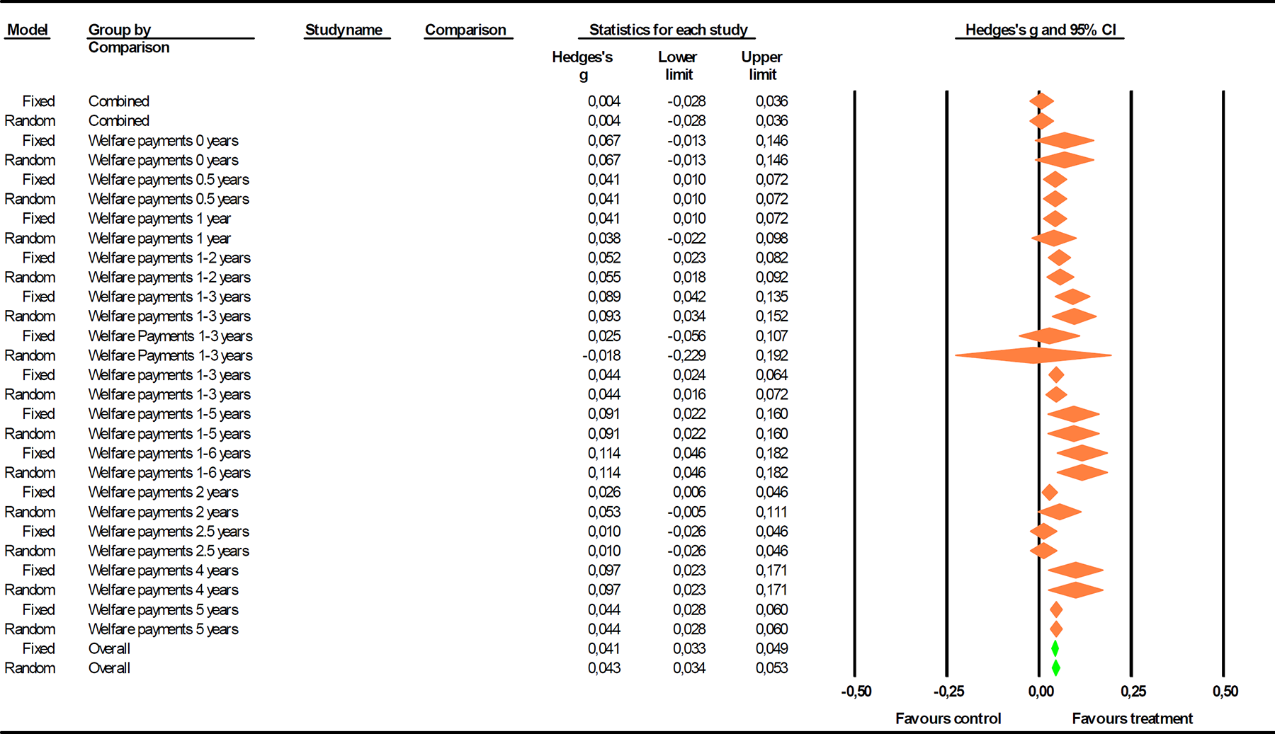
The effect on welfare payments at one year was also small (random-effects Hedges' g = 0.038, 95% CI: -0.022-0.098). At two years, the random-effects g was 0.053 (-0.005-0.111), and at five years the fixed-effects g was 0.044 (0.028-0.060). The programmes reduced the welfare payments from $ 21,719 to $ 18,777 when averaging across all studies. Here the BESD indicated an improvement for 51.2 % of the participants in the intervention groups and for 48.8 % in the control groups.
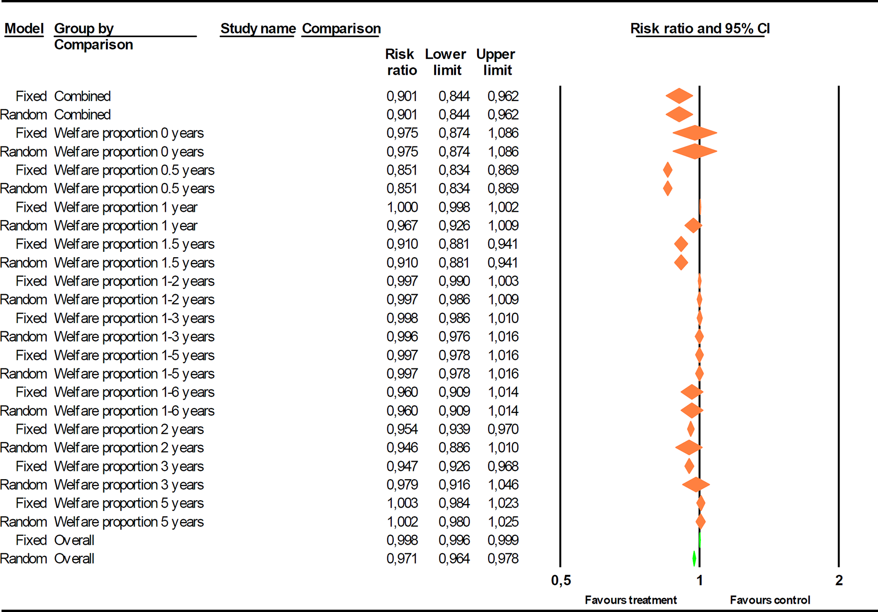
Finally, the effect on the proportion of participants on welfare after one year showed a random effects risk ratio of 0.967 (95% CI: 0.926-1.009). After two years it was of similar magnitude (random-effects RR: 0.946, 95% CI: 0.886-1.010). Finally, after five years, the fixed-effects RR was 1.003 (0.984-1.023). After taking part in a programme, 68 percent (weighted by sample size) were on welfare, compared to 72 percent in the control groups. The overall number needed to treat indicates that, on average, 27 welfare recipients (95% CI: 24-30) had to take part in a programme in order to get an additional person off welfare (overall risk ratio for all outcomes = 0.963, 95% CI: 0.948-0.978).
For all four outcomes, there was significant heterogeneity which could not be sufficiently explained by moderator analysis.
The GRADE quality assessment showed that for all four outcomes, the quality of evidence was very low.
Linked article:
Background
Levitas (1998) distinguished among several discourses about persons outside the labour market. The moral underclass discourse implies a view of welfare recipients as lazy. In this view, if welfare benefits are too generous, recipients will have low motivation to seek employment. This discourse is closely tied to a paternalistic discourse in which the welfare bureaucracy must impose strict work requirements (Dahl 2003). It also blames welfare recipiency on the individual client. There can also be structural causes of welfare recipiency, such as lack of jobs. If the state has an obligation to provide jobs, and the clients are expected to take the available jobs, the relationship between the individual and the state is one of reciprocity. Levitas labelled this the social integrationist discourse.
It is difficult to compare effects of interventions across different countries. Generally, effects vary not only with the nature of the intervention, but also with characteristics of participants, the conditions of the local labour market, and how other welfare institutions are shaped and organised.
Rationale for this review
We are not aware of any systematic reviews of the effects of work programmes for welfare recipients worldwide. Several overviews of controlled trials have been performed (mostly from the USA; Fischer 1995; Michalopoulos, Schwartz, & Adams-Ciardullo 2000; Cebulla et al. 2005; Grogger, et. al. 2002; Bloom, Hill, & Riccio 2003). In Europe, a recent collaborative overview (Cornwell et al. 2002) was performed in six European countries (Denmark, France, Germany, the Netherlands, Norway, and the UK). The results were not directly comparable because the countries have different ways of organising their social services, and they had somewhat different methodological approaches.
The group of individuals on welfare differs among countries. In the USA, welfare is mostly provided to poor families with children. In 1996, the Temporary Assistance for Needy Families (TANF) programme replaced the Aid to Families with Dependent Children (AFDC) as the nation's main welfare programme. Most TANF recipients are single mothers, but there are also some families with two unemployed parents. The Food Stamp Program is also an important transfer programme for the poor in the U. S. In addition there are EITC (Earned Income Tax Credit) and Medicaid. Some countries do not have a sharp distinction between unemployment benefits and welfare benefits, while other countries (for instance Norway and Denmark) distinguish between individuals who are entitled to unemployment benefit if they have been employed in the past, and individuals who are only entitled to welfare. In these countries, all citizens have the right to receive welfare benefit if they have no other source of income.
Objectives of this review
To estimate the effects of work programmes for welfare recipients on work status, earnings, and welfare receipt. To explore sources of heterogeneity. The review tries to identify approaches that appear to be more or less effective overall and, to the extent that adequate data are available, to identify subgroups that are more or less likely to benefit than others. To identify any adverse effects of such programmes (e.g. displacement or negative effect in income or work status).
Methods
Included designs
We chose to limit the review to randomised controlled trials because this is the most rigorous design for studies aimed at establishing causal inference.
Criteria for inclusion and exclusion of studies for this review: Included designs: Randomised controlled trials (RCTs) Cluster randomised trials Quasi randomised trials (allocation not truly random, e. g. using case record numbers, alternation, date of admission, date of birth.)
Excluded designs
Studies using the following designs were collected, listed, and described: Non-randomised concurrently controlled studies (two groups defined by the investigators and dependent variables measured on both groups before and after the intervention) Cohort studies (two groups defined by the interventions and dependent variables measured on both groups before and after the intervention).
There were no restrictions regarding country of publication. There were no language restrictions.
Participants
Welfare recipients. This includes both persons who already receive welfare and people who applied for welfare. People who receive food stamps were also included. We excluded persons entitled to unemployment benefit and persons with pensions of any kind.
Interventions
Interventions intended to help welfare recipients become self-sufficient typically come as “packages” involving several components. Therefore, it is usually not possible to measure the effect of one component apart from the effect of the other components of the programme. We included interventions that offered one or more of the following: time limited work experience, job search assistance, remedial education, job clubs, financial incentives, time limits on financial support, or vocational training. The interventions could be either mandatory or voluntary. In a voluntary programme random assignment takes place after individuals volunteer, and in a mandatory programme volunteering does not take place at all; individuals who meet certain criteria are simply randomly assigned.
The term “time limited work experience” needs some clarification. The work experience is not a permanent job. The duration of the work must be explicitly stated. This duration was recorded for each study.
Control/comparison conditions
The main control or comparison condition was ordinary (passive) social economic assistance or the usual services available to welfare recipients.
Outcome measures
All outcomes involved a comparison between different groups. The comparisons were post intervention measures. Accepted sources of outcome data were state and county administrative records, recordings by programme personnel or employers and self-reports. The type of data source was recorded for each study.
Primary Outcomes: Work status proportion of attendants who obtained competitive work (= work with standard wages and which anyone can apply for). duration of employment during a given time interval. elapsed time until obtained work duration on welfare benefit during a given time interval (as above) proportion on welfare Earnings mean or median earnings at different time points total individual earnings (e.g., income + social insurance + social assistance + welfare benefit) total household earnings Welfare Payments
Secondary outcomes: Skills and satisfaction quality of life social skills self confidence social activity, participation and integration Adverse effects crime drug and alcohol use displacement (when programme participants get jobs, this worsens the chances of non-participants to get jobs) decrease in combined income other
Follow-up durations
Because duration of follow-up was expected to vary across studies, the exact duration of follow-up was recorded for each study. After data collection was finished, duration times were analysed based on the available data. Follow-up times were grouped into “one year”, “two years”, “five years”, “1-3 years” etc.
Search strategy for identification of relevant studies
We searched the following databases: C2-SPECTR (11 December 2003), Cochrane Library (including DARE, CCTR, HTA database (2003 Issue 2), MEDLINE (1966 to November week 3 2005), EMBASE (1980 to 2005 week 47), PsyclNFO (1872 to November week 2 2005), Sociological Abstracts (1963 to November 2003), Cinahl (1982 to November week 3 2005), Caredata (15 September 2003), Eric (1966 to November 2003), SIGLE (for grey literature, 12 March 2003), IBSS (10 March 2004), PAIS (23 March 2004), Dissertation Abstracts International (20031), BIBSYS, and Social Science Citation Index (2003).
The African Trials Registry
Search words in title and keywords were ‘work’, ‘employment’, ‘unemployment’, ‘welfare’, and ‘social assistance’.
We used the same text words across all databases (unless specifically stated) and used the specialised controlled vocabularies for each database. For details of the search strategy, see Appendix A.
Other sources of information
In addition, references from included primary reports were scanned. We also scanned the reference lists from reviews that we found through our search strategy. The following authors of included studies and other potential experts in the field were contacted: Espen Dahl, Ivar Lødemel, Mathematica Policy Research and Abt Associates were contacted by email. Specifically, Gayle Hamilton at MDRC provided comments on a draft version in March 2005. The following centres of the Cochrane Collaboration were contacted by e-mail on 12 January 2006 with a request for trials: Australasian, Brazilian, Chinese, Dutch, German, Italian, Russian (under Nordic branch), South African, and the one in Bahrain. We searched the book “The Digest of Social Experiments” (Greenberg & Shroder 2004). This book documents 240 completed and 21 ongoing social experiments updated until April 2003. Another source of study data is a database of US welfare-to-work programs constructed and maintained by Andreas Cebulla, Stacey Bouchet and David Greenberg (Cebulla et. al. 2005). This database is open to the public and is said to include all known random assignment evaluations of U. S. welfare-to-work programs through 2003 that were targeted specifically at AFDC/TANF recipients.
The following websites were searched: Abt Associates (USA) (Searched 29 November, 2005) Department for Work and Pensions Social Research Branch (UK) (Searched 29 November, 2005) Joseph Rowntree Foundation (UK) (Searched 29 November, 2005) MDRC (USA) (Searched 5 April, 2006) Mathematica Policy Research (USA) (Searched 30 November, 2005) National Centre for Social Research (UK) (Searched 30 November, 2005) RAND Corporation, Social Welfare (USA) (Searched 30 November, 2005) Regard (UK) (Searched 30 November, 2005) Research Forum at the National Center for Children in Poverty (NCCP) (Searched 28 March 2006) Social Work Research Centre (UK) (Searched 30 November, 2005) ( The United States General Accounting Office (USA) (Searched 30 November, 2005) Urban Institute (USA) (Searched 30 November, 2005) U.S. Department for Health & Human Services. Administration for Children and Families (
Criteria for evaluating eligibility of retrieved studies
Two reviewers independently scanned the abstracts and titles of identified reports for eligibility, according to the inclusion criteria above. Full copies of all those deemed eligible by one of the reviewers were retrieved for closer examination. Consensus was reached by discussion and consultation with a third reviewer, if necessary. All studies which initially appeared to meet the inclusion criteria but, based on the full text reports, did not meet the inclusion criteria were detailed in a table of excluded studies.
Quality assessments
We assessed components that may contribute to the measured effectiveness of the included interventions. Two reviewers independently assigned each selected study to quality categories described below. Uncertainty or disagreement was solved by discussion with a third reviewer.
In a properly randomised study, all initial differences between groups will be caused by chance. But these initial differences may be important and can affect outcomes, especially if the study is not large (as N increases, the probability of a meaningful difference between randomised groups decreases). This applies to all prognostic variables, both known and unknown. But in improperly randomised designs and RCTs with differential attrition, there may be important differences between groups. These differences can be systematic, and they can appear in unmeasured variables as well as in the measured ones. It is generally possible to control for the latter but not the former. Matching can be used before the intervention to make groups more similar, and regression methods can be used after the intervention to control for initial differences, but all these methods may introduce bias in the results (Deeks et al. 2003).
Studies, in which both generation and concealment of allocation sequence are MET, were coded as MET below.
MET = Assessor unaware of the assigned treatment when collecting outcome measures. This was also scored as met if the outcome was questionnaire data or data from administrative records.
This review has been graded using GRADE (GRADE Working Group, 2004). GRADE stands for Grading of Recommendations Assessment, Development and Evaluation. The evidence is graded separately for each outcome. Evidence from effect studies is downgraded if the design is not a randomised controlled trial. Limitations might be lack of allocation concealment, lack of blinding, or a large attrition. Consistency refers to the similarity of estimates of effect across studies. Finally, directness refers to the extent to which the people, interventions and outcome measures are similar to those of interest. The overall quality of the evidence is categorised as high, moderate, low, or very low. The reasons for downgrading the evidence are always made explicit in GRADE.
Data management and extraction
Two reviewers independently extracted information from the full text report on study characteristics using a specially designed, pretested data extraction form (Appendix B). For cases in which outcome information was missing from the original reports, attempts were made to retrieve the necessary data for the analysis from the original investigators or from the Internet. For example, missing unemployment rates were collected by going to the website of the U. S. Department of Labor (
Details of study coding categories
Data synthesis
Continuous measures (e.g., earnings) were calculated as standardised mean differences (Hedges’ g). We reported the 95% confidence intervals for all effect estimates. We also reported the post-intervention earnings and welfare payments in US dollars converted to year 2005 equivalents using the following website:
For studies with other currencies, we first converted the amounts into US dollars and then converted to their 2005 equivalents.
We expressed binary outcome measures (e.g., employed/unemployed) as risk ratios (relative risks). The odds ratio is not the correct outcome measure in prospective studies2. We also reported the number needed to treat (NNT, with 95% confidence intervals) for summary findings.
When computing summary statistics, the primary studies were weighted by the inverse of their variance.
We used the advice described in the Cochrane Handbook for Systematic Reviews of Interventions (Higgins 2005) for identifying statistical heterogeneity. If confidence intervals for the results of individual studies (generally depicted graphically using horizontal lines) have poor overlap, this generally indicates the presence of statistical heterogeneity. More specifically we first performed a Chi-square test for heterogeneity. If this approached statistical significance (p < 0.10), we looked at the results of an I-Squared test. If this was greater than 25%, we concluded that there was heterogeneity in the results.
Addressing heterogeneity
When heterogeneity was judged to be large, we examined potential sources using meta-regression, and stratified analyses using categorical moderators.
We performed meta-regressions with the following intervention and contextual moderators: duration of intervention percent sanctioned unemployment in the area during the evaluation years (using, if not found in the report, data from the U.S. Department of Labor, Bureau of Labor Statistics at year when data collection started
The effects of participant characteristics are best measured by looking at separate subgroup results for each primary study (e.g. combining results only for Whites), but this was not feasible because subgroup results were only reported in some of the reports. Instead we entered aggregate data from the primary studies as predictors in meta-regressions: mean age percent of males percent Whites percent Blacks percent Hispanics percent other ethnic group percent with GED (General Educational Diploma) or high school diploma
One moderator was entered at a time, so we could not measure the effect of the moderators controlling for the others (this was not a multiple regression). We report zero-order correlations among the continuous moderators.
We performed separate analyses across the following intervention and setting related factors: labour force attachment (employment-focused) or human capital development (education-focused) strategy job search first or varied first activity mandatory versus voluntary programmes time limits or not financial incentives or not job search/job clubs or not educational intervention or not child care support or not work experience or not skills training or not the current U.S president whether the intervention was conducted before the 1988 Family Support Act (first era), during 1988 through 1995 (second era), or after 19963 (third era). The evaluator of the programme Number of intervention elements (time limits, financial incentives, job search, education, child care, work experience, skills training)
We performed separate analyses across different levels of the following design quality factors: proper generation of the randomisation sequence proper concealment of the randomisation sequence prevention of performance bias prevention of detection bias risk of attrition bias intent-to-treat analysis
To explore possible publication bias, we report a funnel plot for each main outcome showing both observed studies and studies imputed to produce symmetric plots (how it would have looked with no evidence of publication bias).
Sensitivity analyses were used to evaluate whether the pooled effect sizes were robust across different ways of calculating standard errors based on significance levels. Reporting of nonsignificant results was not only analysed using p = 0.1, but also using p = 0.55 and p = 0.99.
Sensitivity analyses were also used for exploring the effects of continuous moderators. For the main analyses, we excluded studies with missing data in the meta-regressions. In another scenario, we imputed the variable means for studies with missing values. We compared the patterns of significant slopes over the two ways of dealing with missing values.
We used fixed effects models when heterogeneity was small (as defined above). We used random effects models when heterogeneity was large, and could not be explained by intervention/setting factors or meta-regression.
Criteria for determination of independent findings
In many instances, several different outcome data are measured on the same subjects in the primary studies (e.g. employment status and earnings). Sometimes the same outcome is measured at multiple points in time. Because these data are from the same sample of participants, and, therefore, are not independent estimates of treatment effect, we analysed the data in such a way that any one analysis contained a single outcome from a particular time period after random assignment. When two intervention groups shared the same control group, we avoided including both intervention groups in the same analysis. Specifically, we used four separate data files for employment, earnings, welfare payments, and proportion on welfare. Within each data file, we grouped the outcomes according to follow-up time. Intervention groups sharing the same control group were not analysed together. The only exceptions were the direct comparisons in Atlanta, Columbus, Grand Rapids, and Riverside, in which we compared two intervention groups sharing a common control group (not a meta-analysis). For the exploratory analyses (meta-regression and the meta-analytic analogue of ANOVA) we used the mean effect magnitude (an option in Comprehensive Meta-Analysis) for studies in which the same outcome was measured at different follow-up times.
Statistical procedures and conventions
Results were analysed using Comprehensive Meta-Analysis software version 2 (Borenstein, et. al., 2004). Prognostic variables were used in analyses if there were less than or equal to 20% missing data. Graphical presentations of effects (forest plots) were produced using Comprehensive Meta-Analysis.
Changes in this review from the published protocol
The main change is that we have extended the inclusion criteria to all programmes that the field perceives as “welfare-to-work” programmes. We previously excluded studies where the programmes did not offer time-limited work experience. But the external reviewers argued that work experience was only a main part of welfare-to-work programmes in the 1960s and 1970s. This component has become less and less important. Wider inclusion criteria are more meaningful and useful for policy purposes.
We have also assessed the quality of the evidence using GRADE (GRADE Working Group, 2004). For each of the four outcomes we graded the evidence for the 2 year follow-up time.
Results
The screening process
Figure 1 is a flowchart of the inclusion process. After having excluded 191 citations from reading the fulltext reports, we were left with 113 citations. Another 45 citations (mainly from Europe) were excluded because they were either nonrandomised controlled studies or they did not include work experience. We included 68 citations when using the limited protocol inclusion criteria. After incorporating the extended inclusion criteria, we included another 34 citations, making the total 102 included citations.
Different endpoints: For some of the 58 conditions there were more than one follow-up time. Because of this, there were e. g. 73 different employment endpoints.
Table 2 (list of excluded studies) consists of 24 citations from 16 studies which were not randomised controlled trials (e. g. cohort studies or nonrandomised studies). Most of these studies were from the United States, but some were from Norway, Belgium, Canada, and the United Kingdom.
Ongoing studies
We identified two ongoing studies which possibly conform to our inclusion criteria:
The first one is a Dutch study (Blonk & Brenninkmeijer 2004) which investigated effects of the JOBS programme in Holland.
The other is the ERA Programme (The Employment Retention and Advancement Program; Anderson & Martinson 2003, 2005). It is conducted in several U. S. sites (Los Angeles County, Riverside County (2), Duval County, Leon County, Cook County, St. Clair County, Medford, Eugene, Hennepin County, New York City (2), and Portland). The programme is also being evaluated in the UK (Walker, et. al., 2006). Over the course of about 15 months, Jobcentre Plus randomly assigned over 16,000 people, making the ERA evaluation the largest random assignment test of a social policy's effectiveness in the UK to date.
Studies awaiting assessment
According to Vasiliy V. Vlassov, director of the Russian branch of the Nordic Cochrane Centre (personal communication, 24 January, 2006), there are a number of Russian databases with free internet access where trials may be described. (A list of databases is at
Raw data
We would like to draw attention to the four included Microsoft Excel files labelled “employment.xls”, “earnings.xls”, “welfare payments.xls”, and “welfare proportion.xls”. The files contain all the raw data collected for this review. There are two reasons for including these files, both having to do with transparency. Firstly, interested researchers will be able to transfer the data into their statistical software package of their likings and check our results, or they may do additional analyses, like multiple meta-regressions. Secondly, anyone having first-hand knowledge of the included primary studies might point out possible errors in the data files or add missing values. Appendix B (data extraction form) provides explanations of the variables in the attached Excel files.
Description of included studies
A main finding is that there are many randomised trials from the United States but few such trials from outside North America (two Canadian programmes were included; see Table 1).
Methodological quality of included studies
Inter-rater reliability
Six raters worked independently and then compared results in pairs. The results reported here were recorded after a pilot test period of the first 12 programmes during which we had meetings and negotiated how to code the studies consistently according to a version of the data extraction form (Appendix B is the latest version). We then coded agreement for 11 programmes4. In total, we coded agreement for 55 variables 11 times, summing up to 605 possible disagreements (Table 3). Note that agreement means different things depending on the type of question. For variables coded “Met”, “Unclear” and “Not Met”, there are six possible ways of disagreeing. For variables such as mean age, there are in principle an infinite number of ways of disagreeing. In such cases, raters had to report exactly the same numerical value in order to get an agreement. The data extraction form (Appendix B) was edited several times during the pilot period, but ultimately all 46 programmes were coded in a consistent way.
For all pairs of raters and all variables we achieved the proportional agreement Po= .82. Table 3 shows in detail how the disagreements were distributed over the 41 variables with disagreement. For the remaining 14 variables5 there was perfect agreement.
Type of design
All included programmes at all sites were reported as randomised controlled trials (although the exact randomisation procedure was not always explicitly reported). Results are for individual sites where these have been reported in such a way that we could calculate an effect size for each site. (For some programmes, e. g. the Food Stamp Employment and Training Programme [53 sites], we could not obtain separate results for each site).
Columns 8-13 in Table 1 show how we judged the reporting of the methodological quality in each programme. In only three instances (EWEP, WDP, Work Program) were all methodological indicators coded as met (truly random allocation, acceptable allocation concealment, prevention of performance bias, prevention of detection bias, prevention of attrition bias, intention-to-treat analysis performed). In five cases all indicators were coded as unclear. There were few cases where the indicators were explicitly not met. (The MASSWEP programme had high attrition. The FIP programme had performance bias, etc.).
In cases where different citations gave conflicting information on the same programme, we gave the authors the benefit of the doubt according to the following rules: If at least one citation was coded as “met”, the whole programme was coded “met” on that variable. But if one citation was “not met” and the rest were “unclear”, the programme was coded as “not met” on that variable.
Prevention of detection bias was met on 48 out of the 58 intervention conditions (Table 4). This was mainly because most studies used state and county records which were defined as being relatively free of this bias.
Prevention of attrition bias was met on 33 conditions because there are systems in place for registering welfare payments, earned income, etc.
Intention-to-treat was explicitly mentioned for 28 of the intervention conditions.
Concealment of the randomisation was met for only 15 conditions, and the proper generation of the randomisation allocation sequence was only met for 10 intervention conditions. It should be stressed that this quality coding refers to the
Finally, prevention of performance bias was met for 21 conditions. This was because in most programmes, the control group participants were free to take part in other programmes while the programme was evaluated. This is only a problem if the purpose of the study is to find the theoretical, counterfactual impact of the intervention. In practice, however, one is often more interested in whether the intervention received by the programme group “adds value” relative to whatever assistance this group would normally have received. Table 4 shows the number and percent of conditions with reports coded as “met”, “unclear” and “not met” for a number of quality indicators.
The GRADE evidence profile (Table 14) concluded that the quality of evidence is very low for all four outcomes. The reasons for this low grading are (1) there are serious limitations in the reporting of the generation of the randomisation sequence and the concealment of this sequence, (2) there is important unexplained inconsistency (heterogeneity) in the results, and (3) there is major uncertainty in the directness of the results because almost all studies are from the USA.
Participants
Our best estimate of the sample size in this systematic review is 412,045 participants, of which 245,509 were randomised to an intervention group and 166,536 were randomised to a control group. Almost 9 out of 10 were women (Table 7). This is because lone parents are usually women. The few males are either unemployed men in two-parent families with small children or heads of single-parent families.
In 1990, the U.S. Bureau of the Census (U.S. Census Bureau 1990) classified race into four major groups: (a) White; (b) Black; (c) American Indian, Eskimo, and Aleut; and (d) Asian and Pacific Islander. According to the 1990 Census, the White population accounted for 82.5 % and the Black population for 12.4 %. The remaining 5.1 percent were in categories (c) and (d). According to Table 7, Black citizens are over-represented and Whites are under-represented in the studies in this review.
Also according to the Census, the percent of people 25 years and over who have completed four years of high school or more rose steadily from 69 percent in 1980 to 84 percent in 2003. Among the participants in this review (some of whom were under age 25), 43 percent had a general educational diploma (GED) and 46 percent had a high school diploma. A GED is received by high school dropouts who pass a qualifying test.
Study participants can also be classified either as recent applicants of welfare when they enter a study, or people who already receive welfare (recipients). Also, they can be divided into single-parent families or two-parent families. We have not taken these distinctions into account in this version of the review, but we might consider doing this in future updates.
Intervention
Table 5 shows that of 73 endpoints6 we classified 46 as employment-focused. Another name for employment-focused is
Nine endpoints (labelled “other”) had a detailed screening process at the outset. The results of this screening influenced whether the participant started job search immediately or began with some kind of educational activity. Finally, in two instances we could not decide what type of intervention focus was in place.
The first activity is closely related to the intervention focus in that employment-focused interventions tend to start with job search assistance, job clubs or work placement, while the education-focused ones usually have more varied first activity, often depending on the job-readiness of the individual client. For 24 endpoints, we coded the intervention as job-search first. For 20 endpoints, we coded varied first activity, and for 26 we coded it as other (Table 5).
Reporting of outcomes
As shown in Table 6, most of the 73 endpoints (N = 46, 63%) had data on earnings and employment from state and county administrative records (register data).
Figures 3 through 6 show meta-analytic summaries of effects grouped according to follow-up time. For each follow-up time, there are two rows that show the fixed-effects and random-effects estimates. A few studies have results for more than one follow-up. These are included in the rows labelled “Combined”. The effect magnitudes with lower and upper bounds of the confidence intervals are shown in the middle part. The schematic on the right is a summary forest plot. The middle of the (orange-coloured) diamonds is located at the estimated effect magnitude, and their widths indicate the length of the 95 percent confidence interval around the estimate. At the bottom, there are two summary rows which give an impression of the overall estimates (with green diamonds). Note that these summaries are meaningful only if the effects do not vary systematically with follow-up time. For proportional outcomes (proportion employed and proportion on welfare) we use risk ratios. The risk ratio is e.g. the relative “risk” of becoming employed. If, for instance, 55 out of 100 in the intervention group become employed and 50 out of 100 in the control group become employed, the risk ratio is 0.55/0.50 = 1.1. A risk ratio of 1.00 indicates no effect. A number greater than 1 indicates that the intervention group is becoming employed to a greater degree, and a number smaller than 1 indicates that the control group is becoming employed to a greater degree.
For continuous outcomes (such as earnings) we use Hedges’ g. A g of zero means no difference between the intervention group and the control group. Large samples usually have more precise estimates than small samples. This precision is measured by the
Each study is weighted by its precision. This means that large and precise studies are given more weight in the analyses. While the confidence intervals for an individual study can be wide, the meta-analysis confidence intervals are much narrower, signalling a more precise estimate.
Heterogeneity is a measure of the spread of results. Statistical tests of homogeneity (i.e. lack of heterogeneity) assess whether the individual study results are likely to reflect a single underlying effect, as opposed to a distribution of effects. If this test fails to detect heterogeneity among results, then it is assumed that the differences observed between individual studies are a consequence of sampling variation and simply due to chance.
Impact on employment, earnings, welfare payment, and proportion on welfare
Impact on Employment
Figure 3 shows the impact on employment graphically for all follow-up lengths. Each follow-up time has two separate meta-analyses (fixed-effects and random-effects). Thus, there are two separate meta-analyses for ‘employment 2 years’ and two others for ‘employment 1-3 years’. Figure 3 shows that the employment at 1 year random-effects risk ratio is 1.097 (95% CI: 1.006-1.196). The employment at 2 years random-effects risk ratio is 1.092 (95% CI: 1.032-1.157), and the five year random-effects risk ratio is 1.037 (1.004-1.071). Homogeneity tests show that, in addition, the following follow-up times should use random-effects summaries: 0.25 years and 1-3 years. The remaining follow-ups were homogeneous and should use fixed effects.
There are three overall impressions: (1) Effects are more and less consistently in favour of the intervention group; (2) effects vary, and (3) effects are small. The intervention group does better than the control group, but the effect is small. The overall effects are heterogeneous (Qall studies = 414.967, df = 59, p = .000, I2 = 85.8).
Overall, 60.9 percent of intervention participants (weighted by sample size) were employed at the follow-ups. But 57.9 percent of control participants were also employed. Another way to look at these results is to compute the number needed to treat (NNT). The absolute risk reduction (ARR) was 0.609 - 0.579 = 0.03. The number needed to treat was 1/ARR ≈ 33 (95% confidence interval: 30-37). This was estimated by first computing the confidence limits for the ARR7 and computing the confidence limits for the NNT as the reciprocals of the ARR confidence limits. In other words, an average of 33 welfare recipients had to receive one of the work programmes in this review in order to predict employment of one more recipient.
When 54 employment outcomes were ranked according to effect size, the GAIN programme in Riverside ranked in 6th place, while the same intervention in Alameda, Los Angeles, San Diego, Tulare, and Butte ranked 9, 13, 21, 28, and 47, respectively. This is an indication that the local context in which a programme is executed has a more powerful effect on the outcome than the programme itself.
Impact on Earnings
Because few studies reported the standard errors necessary for direct computation of Hedges’ g, we had to use p-values to estimate most of the standard errors. This was the only way to estimating effect sizes. Only a few studies reported exact p-values. If a standard error was reported, we used it. If not, we used p-values. If an exact p-value was reported, we used this value. Otherwise, we used the following conversion:
The included studies mostly used p = 0.1 as the critical value for choosing between significant/not significant. We decided that any other value of p would be arbitrary. This probably caused some comparisons reported as nonsignificant to have caused an upward bias to effect-magnitudes. Therefore we ran two sensitivity analyses. In that way, we established a range of probable results. In the first scenario we used p = 0.99 for nonsignificant findings. In the second scenario, we used p = 0.55 (midpoint between 0.1 and 1.0) for nonsignificant findings.
The rationale is simply that this value is half way between 0.1 and 0.05.
This value is half the way between 0.05 and 0.01
Every smaller value would be arbitrary. This causes some comparisons with very low p-values to be underestimated. However, some exploratory analyses with extremely small p-values (not shown) did not change the estimated effect size to any large degree.
Figure 4 shows the impact on earnings. Overall, the intervention groups did slightly better than the control group, but the difference was small. The results are heterogeneous (Q = 180.96, df = 65, p = .000, I2 = 64.1). At the one-year follow-up, the random-effects Hedges’ g was 0.043 (95% CI: 0.011-0.076). At two years the random-effects g was 0.044 (0.022-0.066), and at five years the random-effects g was 0.011 (-0.029-0.050). Apart from these, the 1-3 years analysis should also use random effects.
Sensitivity analyses showed that using p = 0.99 for nonsignificant results lowered the overall g from 0.047 to 0.032 (0.022-0.042), and that using p=0.55 produced a g of 0.035 (0.024-0.045). The three confidence intervals overlap, and, hence, we used p=0.1 for all nonsignificant analyses.
The mean earnings (in year 2005 US dollars) across all the intervention outcomes were $ 11,021 compared to $ 8,843 in the control groups. Two studies were conducted in Canada. We converted the Canadian dollars into US dollars using the exchange rate of 1CAD = 0.873 USD (17 April, 2006).
Using the Binominal Effect Size Display (BESD8) the results roughly correspond to a positive effect for 51.1 % in the intervention groups and for 48.9 percent in the control group.
On a ranked list of 64 effect magnitudes, the different sites at which the GAIN programme were implemented ranks 5, 18, 29, 36. 43 and 44. Similarly, the NEWWS evaluation sites rank 12, 13, 14, 24, 25, 27, 28, 33, 38, 41, and 57. This is again an indication that aspects of local implementation may matter more than the programme model itself (note that these comparisons are inherently quasi-experimental).
Impact on Welfare Payments
Figure 5 shows the impact on welfare payments. Once again, the intervention group mostly does better than the control group (the intervention group receives less welfare payments), but the effect is small (overall random effects Hedges’ g = 0.043, 95% CI: 0.034-0.053). The results are heterogeneous (Q = 105.7, df = 42, p = .000, I2 = 60.3). At one year follow up the random-effects g was 0.038 (95% CI: -0.022-0.098). At two years, the random-effects g was 0.053 (-0.005-0.111), and at 5 years the fixed-effects g was 0.044 (0.028-0.060). The 1-3 years follow-up was heterogeneous and should use random effects.
The BESD indicates that 51.2 percent in the intervention groups and 48.8 percent in the control groups would receive less welfare payments as a result of taking part in a programme.
Using p = 0.99 for nonsignificant results reduces g from 0.043 to 0.040 (0.026-0.053), and using p = 0.55 estimates g to be 0.042 (0.029-0.055). Again, the CI's overlap, and we used p = 0.1 for all nonsignificant analyses.
On a ranked list of 43 effect magnitudes, the sites of the GAIN evaluation rank 7, 13, 20, 22, 29, and 39. The California Work Pays evaluation sites rank 2, 14, and 25.
Impact on Welfare Proportion
Figure 6 shows the impact of the programmes on the proportion of people who were still receiving welfare at the follow-ups. Note that “favours treatment” is on the left side. Overall, the intervention groups do slightly better than the control groups (the intervention group participants are less likely to be on welfare at the follow-up), but the effect is small. At the one-year follow-up, the random-effects risk ratio is 0.967 (95% CI: 0.926-1.009). At two years, the random-effects risk ratio is 0.946 (0.886-1.010), and at five years, the fixed-effects risk ratio is 1.003 (0.984-1.023). The results for the 1-2 years and the 3 years follow-ups were also heterogeneous. The overall results are heterogeneous (Q = 529.292, df = 38, p = .000, I2 = 92.8). Overall, the proportion of intervention participants living on welfare at the follow-ups was 68.4% compared to 72.1% in the control groups. This gives an absolute risk reduction of 0.037 and a NNT of 27 (95% confidence interval 24-30).
On a ranked list of 40 effect magnitudes, the California Work Pays evaluation sites rank 10, 18, and 37.
The differential effect of employment focus and education focus
As part of the JOBS (NEWWS) evaluation, in three sites (Atlanta, Grand Rapids and Riverside), subjects were randomised into either a HCD (human capital development) condition, a LFA (labour force attachment) condition, or a control condition.
Employment: A random-effects meta-analysis at the three sites showed that the LFA approach had a slightly better effect on employment (risk ratio: 1.094, 95% CI: 1.056-1.133) than the HCD approach (risk ratio: 1.049, 95% CI: 1.003-1.098), but the confidence intervals have a large overlap. Overall, the results were heterogeneous (Q = 25.7, df = 5, p = .000, I2 = 80.5). The subgroups were also heterogeneous (HCD: Q = 8.7, df = 2, p = .013, I2 = 76.9 / LFA: Q = 4.8, df = 2, p = .087, I2 = 59.0)
No direct comparisons on the effects on earnings, welfare payments or welfare proportion were available for the LFA and HCD approaches.
Integrated or traditional case-management
At Columbus, Ohio the participants were randomised into either a traditional case management approach or an integrated approach. In the traditional case management model, welfare eligibility and employment programme functions were performed by separate staff members. In the integrated case management model, these two functions were performed by the same staff member. At two years the two approaches generated almost exactly the same earnings that were also close to the control group (integrated: Hedges’ g = 0.076, 95% CI: 0.018-0.133, traditional: Hedges’ g = 0.075, 95% CI: 0.018-0.132. At five years, the approaches did not have a statistically significant effect on employment, and neither did they differ (integrated: risk ratio = 1.022, 95% CI: 0.999-1.045, traditional: risk ratio = 1.012, 95% CI: 0.989-1.035.
Publication bias
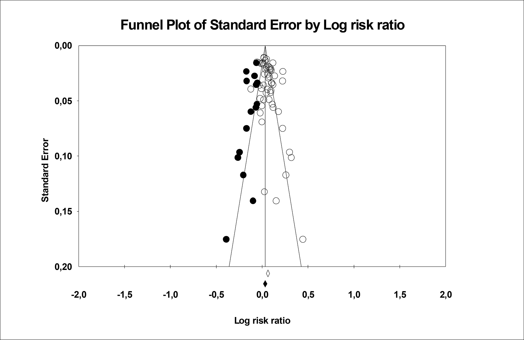
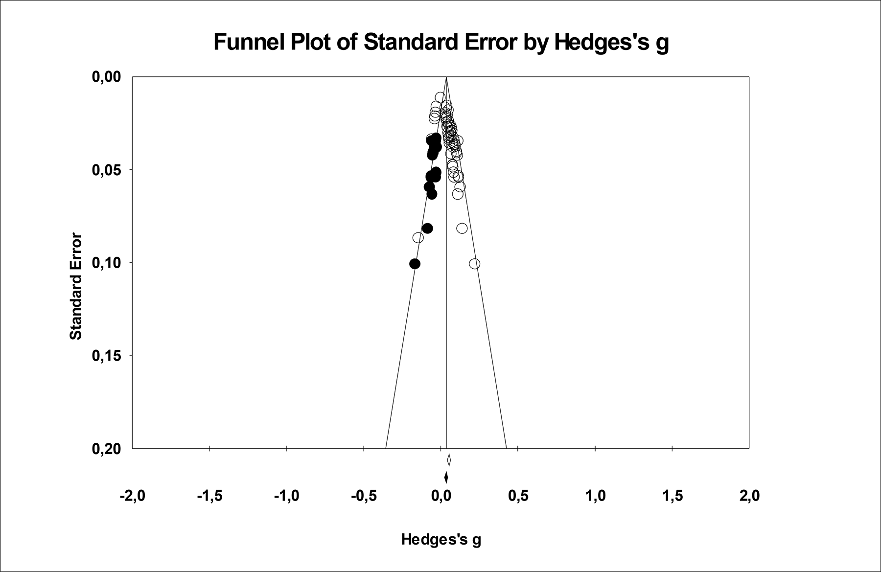
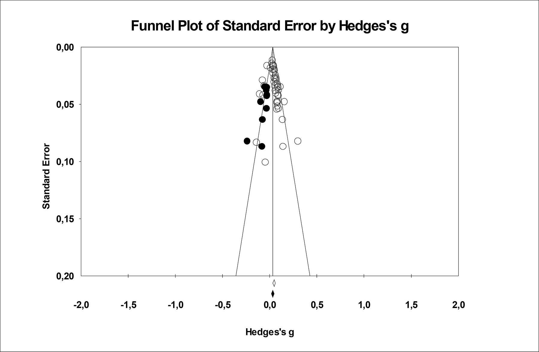
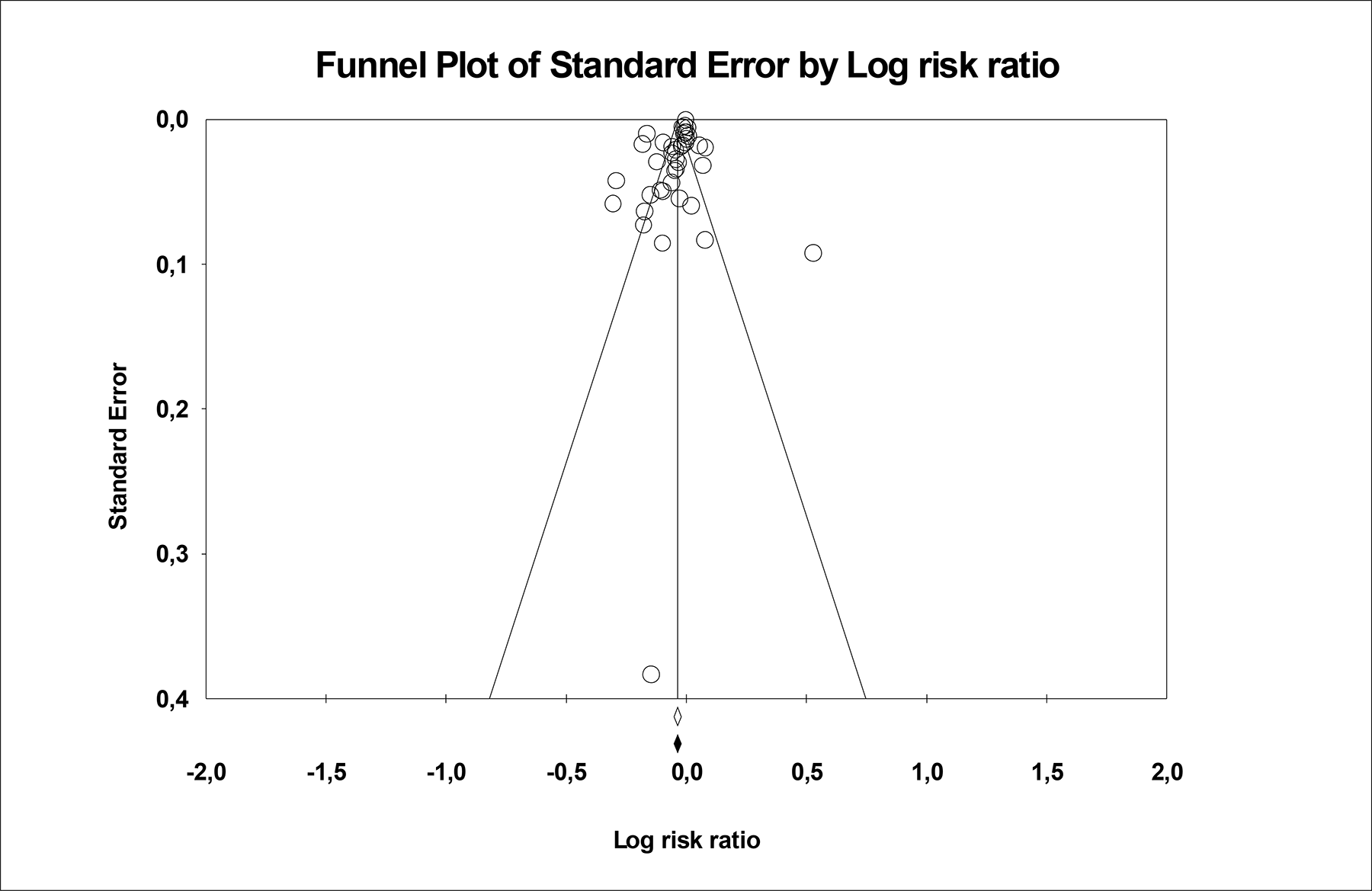
Figures 7–10 are funnel plots showing for each of the four outcomes the relation between each study's effect size and its standard error. In the absence of publication bias the studies will be distributed symmetrically about the combined effect size. By contrast, in the presence of bias, the bottom of the plot would tend to show a higher concentration of studies on one side of the mean than the other. This would reflect the fact that smaller studies (which appear toward the bottom) are more likely to be published if they have larger than average effects, which makes them more likely to meet the criterion for statistical significance. We have used a “trim and fill” function which builds on the key idea behind the funnel plot; that in the absence of bias the plot would be symmetric about the summary effect. If there are more small studies on the right than on the left, the concern is that studies may be missing from the left. The trim and fill procedure imputes these missing studies, adds them to the analysis, and then re-computes the summary effect size. Figures 7–10 indicates that there is some asymmetry in the plots for employment, earnings, and welfare payments, but not for welfare proportion.
Exploratory moderator analyses
Because the results were heterogeneous, we attempted to explore this heterogeneity using moderator analyses. Note that by doing this, randomisation is lost, and, hence, the following are quasi-experimental results. Also note that they are exploratory hypothesis-generating analyses. They are not theory-driven, hypothesis-testing analyses.
Data on a number of variables were collected, but not used as possible moderators. Country where the study was conducted was e.g. not used because all but two studies came from the USA. For the same reason, publication type was not used because the majority of citations were reports. Publication year was not used because we used the year when the data collection started. Design was not used, since all studies used RCT. Some potentially interesting variables were not used because of a large number of missing values (number of children, age of youngest child, previous work experience, previous welfare history, extent of work experience). Finally we did not use data on funding and implementing agents. Studies were mostly funded and implemented by federal and state authorities.
Continuous moderators
Table 7 provides descriptive data on continuous moderators. Table 8 shows the zero-order, non-parametric Spearman correlations among moderators.
Tables 9 through 12 show the results of meta-regressions using the continuous moderators. As indicated above, one moderator was entered into these regressions at a time; thus, these are bivariate (not multivariate) regressions that do not control for influences of other moderators.
Table 9 shows for instance that if, for example, the mean age in a study is raised by one year, the proportion becoming employed is expected to be 0.8 percentage points higher (slope: 0.00829). In the following we list the regressions where the 95 percent confidence interval for the regression slope does not cross the point of no effect. An asterisk is also listed at the end of these variable names in the tables. All in all, there were 48 such comparisons. We also note the deviations from this pattern in the sensitivity analyses using imputation of the mean for missing data.
Employment (Table 9)
Positive associations: mean age, percent other ethnic group, duration of intervention, and regional unemployment. Negative associations: proportion of Whites, proportion of Blacks, and percent sanctioned In the sensitivity analysis, proportion of Hispanics also showed a positive association.
Earnings (Table 10)
Positive association: proportion of Blacks Negative associations: year when data collection started, proportion of Whites, proportion of Hispanics, and proportion with a general educational diploma or high-school degree. In the sensitivity analysis, proportion sanctioned showed a negative association. We also failed to reproduce the negative association with GED.
Welfare payments (Table 11)
Negative associations: proportion of males, proportion of Whites In the sensitivity analysis, duration of intervention showed a positive association.
Welfare proportion (Table 12)
Negative associations: mean age, proportion of males, proportion of Hispanics, proportion of other ethnic group, duration of intervention, proportion sanctioned, regional unemployment, and number of intervention elements. In the sensitivity analysis, we also found a positive association with proportion of Blacks, and a negative association with proportion of Whites.
The proportion of males, proportion of Whites, and percent sanctioned have negative slopes for all outcomes, but these slopes are not always statistically significant. These findings indicate (but only very weakly) that the programmes might have been more effective for women, and for non-Whites, and that programmes with less sanctioning have been more effective. For the other variables, the direction of the slope varies. The sensitivity analyses found five additional significant slopes (11%), while one significant slope (2%) in the main analysis was not significant in the sensitivity analysis.
For all regressions, the residual Q was significant at p = .00000. This indicates that any single moderator explains only a very small part of the variability in effect magnitudes.
Categorical moderators
Tables 13 through 20 show the effects of categorical moderators on employment, earnings, welfare payments, and welfare proportion. An asterisk is listed at the end of the variable name if the between-group heterogeneity p-value is below 0.05. These are interpreted as statistically significant differences among the categories of moderators.
Table 13 shows the separate risk ratios for each level of the design quality variables regarding effect on employment. The number (k) of outcomes contributing to each level is shown first. For example: we coded 12 outcomes as “Met” on random allocation. The separate metaanalysis for these outcomes showed a risk ratio of 1.064 with a 95 percent confidence interval from 1.016 to 1.115. This risk ratio was significantly different from zero (p = .008). The Qwithin groups was 53.9 and the I-squared was 79.6. The Qbetween groups was 26, which shows that this meta-analytic analogue of ANOVA is significant. In other words, the effect magnitude varies over the different quality ratings of random allocation. Specifically, studies coded as “Not Met” have smaller risk ratios than studies coded as “Met” and “Unclear”.
Tables 15, 17, and 19 do the same as Table 13 for the effects of design characteristics on earnings, welfare payments and welfare proportion.
Overall, these analyses show that “Not Met” and “Unclear” are associated with very high or very low effect magnitudes. High-quality reporting (Met) is associated with larger effect magnitudes in 54% (13/24) of the comparisons. The “Unclear” category had strongest effects in 21% of the comparisons (5/24), and the “Not Met” category had strongest effect sizes in 25% (6/24) of the comparisons.
A coding of “Met” on allocation concealment is always associated with the largest effect magnitude (although the difference was not always statistically significant).
Tables 14, 16, 18, and 20 show estimated effects of the other categorical variables on employment, earnings, welfare payments and welfare proportion.
Other consistent findings: Voluntary programmes show larger effects than mandatory programmes, but differences are not statistically significant. Programmes with work experience show larger effects than the ones without work experience (again differences are not always significant). Programmes with job search show larger effects than programmes without job search.20
We note once more that these associations are not of a causal nature and should be taken only as exploratory analyses.
Discussion
A major finding of this review is that randomised effect evaluations of welfare-to-work programmes come almost exclusively from the USA. Why is this so? In the USA, having a randomly allocated control group has sometimes been a condition for receiving money to evaluate a programme. But randomisation has also sometimes been a condition for receiving federal waivers that allow proposed programmes to go forward. The latter has probably been more important in stimulating the use of random assignment in the United States than the former.
In Europe, randomisation is often regarded as unethical, because the control group is denied a possibly beneficial intervention. In the United States this is not looked upon as a problem. In fact, they argue, whenever only some of the welfare recipients can receive a programme, random allocation is the fairest way of sharing these scarce resources. It has also been claimed that not using the best design is unethical because if not, one will never learn whether the intervention works, is ineffective or harmful. “Possibly beneficial” interventions are not necessarily beneficial and may, in fact, be harmful; and we will not know whether something is beneficial or harmful until we do randomised controlled trials.
For welfare recipients, the programmes only have a net effect if it can raise their total income. This occurs only if the increase in earnings is greater than the reductions in welfare payment. Cost-benefit analysis is not part of the present review though.
Some readers of the welfare-to-work literature may be unfamiliar with the reporting of results as effect sizes. They are used to having results presented in their original metrics (such as dollars for earnings and percent for employment). We have attached all the collected data (as Microsoft Excel files) in Appendix C. For each study and outcome the proportion employed or on welfare is listed, and the dollar amounts in 2005 equivalents are used for continuous measures. We invite readers to examine these data.
The two Canadian programmes (SSP and SSP+) seem to perform somewhat better than the US programmes according to a ranking of effect sizes. On a list of 54 employment outcomes, SSP+ places second and SSP places fourth. On a list of 44 welfare payment outcomes, SSP+ is the “winner”, while SSP is at place 19. Finally, on a list of 36 welfare proportion outcomes, SSP places second. Again, these are only quasi-experimental comparisons.
Reviewers’ conclusions
Implications for practice
Implications for research
Plans for updating the review
Potential conflicts of interest
Contributions and acknowledgements
Thanks to Espen Dahl and Ivar Lødemel for giving advice as content experts and commenting on parts of drafts. Thanks to Sari Susanna Ormstad for running an updated literature search in November 2005. Thanks to Gunn Elisabeth Vist for help with grading the outcomes.
INCLUDED CITATIONS
EXCLUDED CITATIONS
ADDITIONAL REFERENCES
Tables and Figures
Overview of the 46 included programmes
Excluded Non-randomised programmes/references with descriptions (16 programmes)
Variables (n = 41) with disagreement
Quality coding of the included programmes (58 sites)
Description of interventions by endpoint (n = 73)
Type and reporting of outcomes by endpoint (n = 73)
Descriptive data on all recorded continuous moderators
Zero-order correlations15 among the continuous moderators
Effects of Continuous Moderators on Employment (meta-regression)
means that the 95% confidence interval for the regression slope does not cross zero; the moderator has a statistically significant effect for that outcome.
Effects of continuous moderators on earnings
Effects of continuous moderators on welfare payments
Effects of continuous moderators on welfare proportion
Effects of design quality moderators on Employment
means that differences are statistically significant.
Effects of categorical moderators on employment
Effects of design quality Moderators on Earnings
Effects of categorical moderators on earnings
Effects of design quality moderators on welfare payment
Effects of categorical moderators on welfare payments
Effects of design quality moderators on welfare proportion
Effects on categorical moderators on welfare proportion
Table 14. Grading of the outcomes
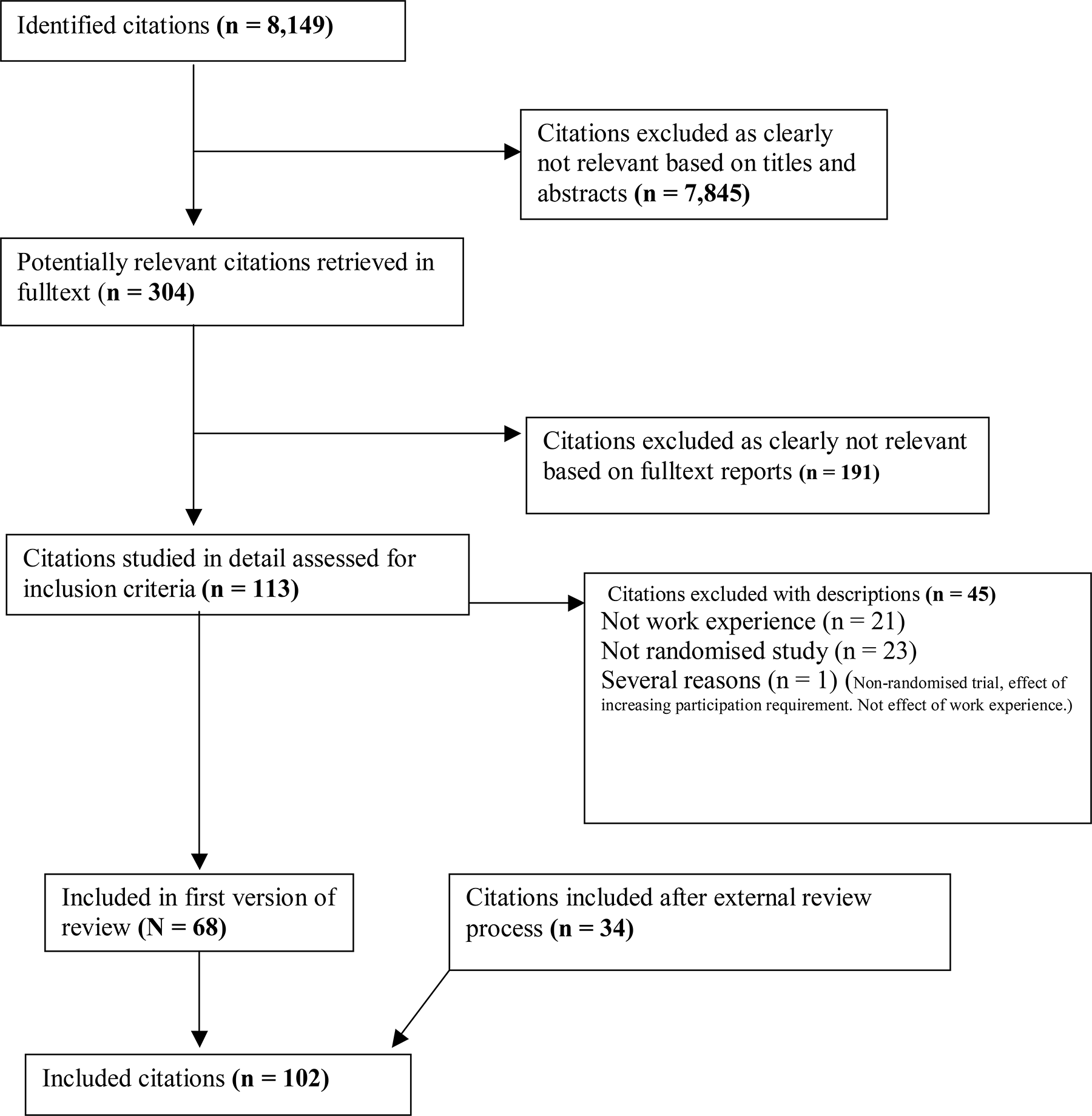
Selection process of eligible randomised controlled trials from all identified citations
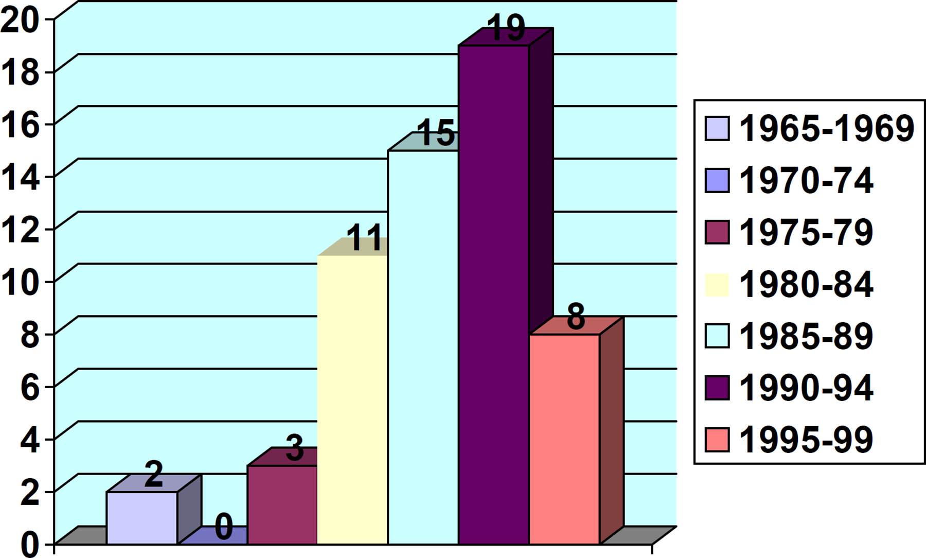
Year when data collection started (n = 58 intervention sites)
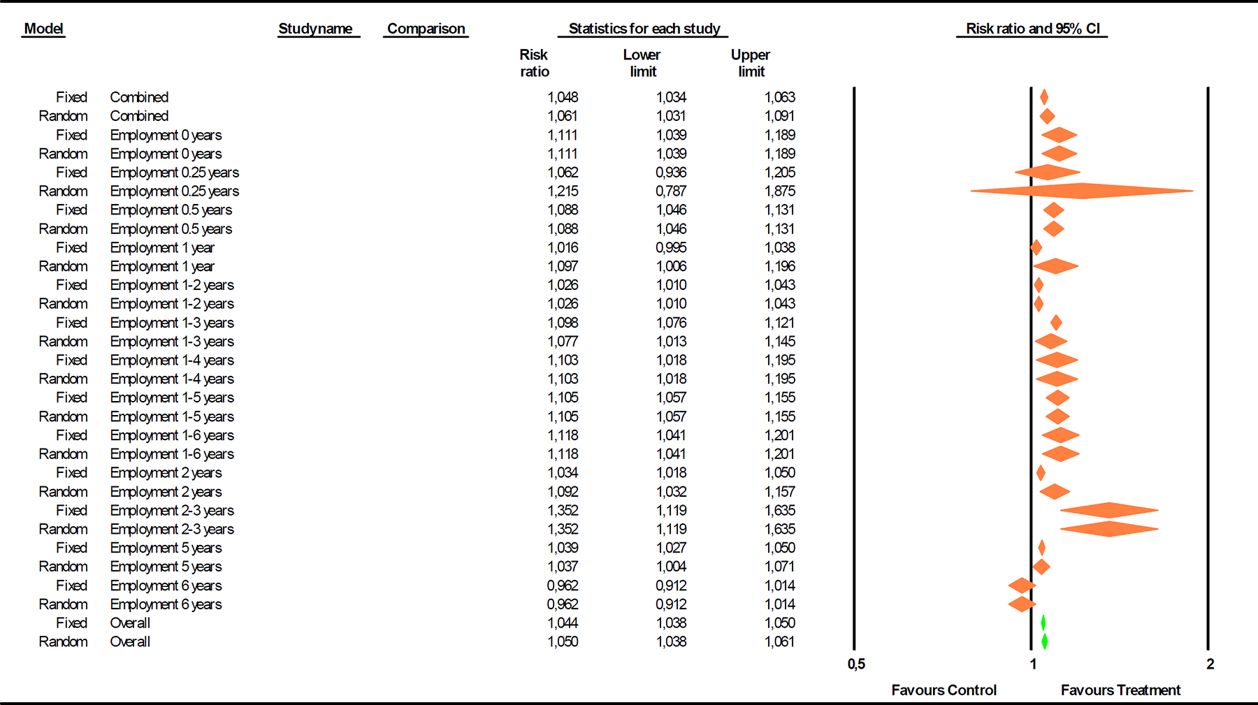
Effects on employment
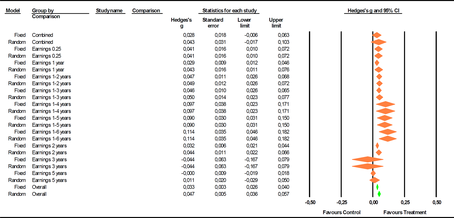
Effects on earnings
Effects on welfare payments
Effects on welfare proportion
Employment publication bias.
Funnel plot of log risk ratio against its standard error. Open circles signify the actual studies. Closed circles are virtual imputed studies that would be expected if there were no publication bias present in the data.
Earnings publication bias.
Funnel plot of Hedges’ g against its standard error. Open circles signify the actual studies. Closed circles are virtual imputed studies that would be expected if there were no publication bias present in the data.
Welfare payments publication bias.
Funnel plot of Hedges’ g against its standard error. Open circles signify the actual studies. Closed circles are virtual imputed studies that would be expected if there were no publication bias present in the data.
Welfare proportion publication bias.
Funnel plot of the log risk ratio against its standard error. Open circles signify the actual studies. Closed circles are virtual imputed studies that would be expected if there were no publication bias present in the data.
Footnotes
Appendix A
Appendix B
1
Unfortunately, the exact dates of search in this database, BIBSYS, and Social Science Citation Index were lost.
2
Altman, Deeks, and  wrote, “The odds ratio is valuable in case-control studies where events are usually rare and the relative risk cannot validly be estimated directly. In prospective studies interpretation of the odds ratio as an approximation to the relative risk becomes unreliable when events are common, and thus its use for prospective studies, especially randomised trials and systematic reviews, has been criticised. The distortion is especially large when the event rate is high in only one group. The odds ratio should not be interpreted as an approximate relative risk unless the events are rare in both groups (say, less than 20-30%). The odds ratio remains especially useful when researchers need to adjust for other variables, for which logistic regression is the usual approach. While such analyses are valid, when the objective is to communicate study results to an audience unfamiliar with the relation between odds ratios and relative risks, surely it makes no sense also to report the relative risk when this differs markedly from the odds ratio.”
3
The Personal Responsibility and Work Opportunity Reconciliation Act (PRWORA) marked the transition from the older AFDC system to the newer TANF). AFDC stands for Aid to Families with Dependent Children, and was operated between 1937 and 1995. TANF stands for Temporary Assistance for Needy Families. Key elements of TANF include a lifetime limit of five years (60 months) on the amount of time a family with an adult can receive assistance funded with federal funds, increasing work participation rate requirements which states must meet, and broad state flexibility on program design.
4
5
Main reference, publication type, publication status, publication year, design type, control variables, proportion of Hispanics, mean years of education, broadness of enrolment, degree of monitoring, table/figure where outcome was reported, sample size in intervention group number 3, sample size in intervention group number 4, sample size in control group number 3.
6
“Endpoints” refer to sites with separate results. Studies with one site report only one endpoint, whereas a study with e. g. seven sites is listed here with seven endpoints.
7
Standard deviation for
8
BESD shows the proportion in the intervention group with a positive result as 0.5 + r/2 and the proportion in the control group with positive result as 0.5 - r/2. First we had to convert the standardised mean difference into r.
9
M= MET, U=UNCLEAR, N=NOT MET, EP= employment-focused, ED=education-focused, OT = other than employment-focused or education-focused, J=job search first, V=varied first activity.
10
“30+1/3.” Is a federally allowable earned income disregard provision which disregard $30 plus 1/3 of the remaining income and bases the grant on that. The 100-hour rule means that families with an unemployed parent (AFDC-U) were ineligible for AFDC if the father worked 100 hours or more in a month.
A. 11
“Graduated stress” allows participants to adjust to major changes through transitional processes. This technique promotes success through gradual adaptation and the strategic use of supports. It can be used, for example, to transition participants from lower levels of work activity to full time equivalent hours (a new state requirement). It can also be used to move people from program participation to unsubsidized employment by providing strong post-placement supports for both the employer and the new employee.
12
“Caseload saturation,” i.e., having as many persons participate in activities for as long as possible.
13
PROBABLY SEVERELY FLAWED! Only earnings data from the welfare recipients themselves. As a result, the evaluators were limited to non-experimental comparisons of only those cases that were active on welfare.
14
The quality indicators are explained in the protocol.
15
Non-parametric correlations were used because the variables were not normally distributed.
Supplementary Material
Please find the following supplemental material available below.
For Open Access articles published under a Creative Commons License, all supplemental material carries the same license as the article it is associated with.
For non-Open Access articles published, all supplemental material carries a non-exclusive license, and permission requests for re-use of supplemental material or any part of supplemental material shall be sent directly to the copyright owner as specified in the copyright notice associated with the article.
