SPATIAL DISPLACEMENT AND DIFFUSION OF BENEFITS AMONG GEOGRAPHICALLY FOCUSED POLICING INITIATIVES 1

Abstract

Overall, teachers' multi-component classroom management programmes have a significant positive effect in decreasing aggressive or problematic behaviour in the classroom. Students in the treatment classrooms in all 12 studies reviewed showed less disruptive or problematic behaviours when compared to the students in control classrooms without the intervention. It is not possible to make any conclusions regarding what components of the management programmes are most effective due to small sample size and lack of information reported in the studies reviewed.

STRUCTURED ABSTRACT

Background

One of the most common criticisms of spatially focused policing efforts (such as Problem-Oriented Policing, police ‘crackdowns’ or hotspots policing) is that crime will simply relocate to other times and places since the “root causes” of crime were not addressed. This phenomenon—called crime displacement—has important implications for many policing projects. By far, spatial displacement (movement of crime from a treatment area to an area nearby) is the form most commonly recognized. At the extreme, widespread displacement stands to undermine the effects of geographically focused policing actions. More often, however, research suggests that crime displacement is rarely total. On the other end of the displacement continuum is the phenomenon of ‘diffusion of crime control benefits’ (a term coined by Ron Clarke and David Weisburd in 1994). Diffusion occurs when reductions of crime (or other improvements) are achieved in areas that are close to crime prevention interventions, even though those areas were not actually targeted by the intervention itself.

Objectives

To synthesize the evidence concerning the degree to which geographically focused policing initiatives are related to spatial displacement of crime or diffusion of the crime control benefits.

Search Strategy

A number of search strategies were used to retrieve relevant studies. First, we undertook a keyword search of electronic abstract databases. Second, we searched bibliographies of existing displacement reviews and reviews of the effectiveness of focused policing initiatives. Third, we did forward searches for works that had cited key displacement publications. Fourth, we reviewed research reports of professional research and policing organizations. Fifth, we undertook a hand search of pertinent journals and publications. Finally, once these searches were all completed we emailed a list of the studies that we had assessed as meeting (and a separate list of those not meeting) our criteria to a number of key scholars with knowledge of the area to identify any further studies we might have missed.

Selection Criteria

Eligible studies met the following criteria; (1) they evaluated a policing initiative; (2) this initiative was geographically focused to a local area; (3) the evaluation included a quantitative measure of crime for both a ‘treatment’ area and a displacement/diffusion ‘catchment’ area. This needed to be available for both a pre- and a post- (or during-) intervention period. Other criteria specified that the study was written in English and that it reported original research findings. The studies could have been conducted at any point in time and at any location. Both published and unpublished studies were included.

Data Collection and Analysis

For all of our 44 eligible studies, we produced a narrative review and a summary of the author's findings, concerning the effectiveness of the policing initiative and any displacement or diffusion observed. For the 16 studies for which we were able to gain pre and post measures of crime for each of a minimum of three area types (a treatment, control and catchment area) we produced odds ratio effect sizes which were used in a meta-analysis. For the meta-analysis we reported the mean effect size for both the treatment areas and the catchment areas. This summarized the effectiveness of the policing interventions and the displacement/diffusion effect respectively. Because a number of studies had more than one primary outcome, we reported the largest effect and the smallest effect in each case. We also performed permutation tests using combinations in which one primary outcome was chosen from each study. Other tests assessed the effects of study design, intervention type, size of intervention and publication bias. A further quantitative analysis of these 16 studies summarised the mean Weighted Displacement Quotient (WDQ) a measure developed in earlier work by two of the study authors. Finally, a proportional change analysis looked at increases and decreases in crime in treatment and catchment areas for the 36 studies for which count data were available. This analysis did not require data to be available for a control area.

Main Results

For the weighted displacement quotient analyses, the weight of the evidence suggests that where changes are observed in catchment areas that exceed those that might be expected in the absence of intervention, a diffusion of crime control benefit rather than displacement appears to be the more likely outcome.

The results of the proportional change analysis suggest that the majority of eligible studies experienced a decrease in crime in the treatment area indicating possible success of the scheme. The majority also experience a decrease in the catchment areas suggesting the possibility of a diffusion of benefit. These findings, which could not be statistically tested, are consistent with all others reported here, and with those from the narrative review.

Conclusions

In summary the message from this review is a positive one to those involved in the sort of operational policing initiatives considered, the main point being that displacement is far from inevitable as a result of such endeavor, and, in fact that the opposite, a diffusion of crime control benefits appears to be the more likely consequence.

1. Background⁴

One of the most common criticisms of focused policing efforts is that crime will simply relocate to other times and places since the “root causes” of crime were not addressed or because offenders may remain on the streets after certain crime opportunities are reduced. This phenomenon—called crime displacement—has important implications for many policing projects. By far spatial displacement is the form most commonly recognized (Eck, 1993), though the other five are also frequently acknowledged by those studying crime prevention. Formally, the six possible forms of displacement include: temporal (offenders change the time at which they commit crime), spatial (offenders switch from targets in one location to targets in another location), target (offenders change from one type of target to another target type), tactical (offenders alter the methods used to carry out crime), offense (offenders switch from one form of crime to another), and offender⁵ (new offenders replace old offenders who have been removed or who have desisted from crime).⁶ At the extreme, widespread displacement stands to undermine the effects of geographically focused policing actions. More often, however, emerging research suggests that crime displacement is rarely total. On the other end of the displacement continuum is the phenomenon of diffusion of crime control benefits (Clarke and Weisburd, 1994). Crime diffusion is the reverse of displacement and its occurrence has been documented in several crime prevention evaluations (Bowers and Johnson, 2003; Chaiken, Lawless, and Stevenson, 1974; Green, 1995; Miethe, 1991; Weisburd et al., 2006; Weisburd and Green, 1995). Diffusion occurs when reductions of crime (or other improvements) are achieved in areas that are close to crime prevention interventions, even though those areas were not actually targeted by the intervention itself (Clarke and Weisburd, 1994). This feature of crime prevention activity has been referred to in a variety of ways including the “bonus effect,” the “halo effect,” the “free-rider effect,” and the “multiplier effect.” In cases where any degree of diffusion is observed the benefit of any treatment effects experienced in the targeted area are amplified since improvements were gained without expending resources in those areas. While there have been some noted experiments on the extent of displacement and diffusion following focused policing efforts which suggests this is the case, a systematic appraisal of all the available evidence on this topic remains missing.

Overall, displacement is viewed as a negative consequence of crime prevention efforts, but even when displacement does occur it can still provide some benefit. For example, the volume of crime shifted could be less. A treatment area may experience a reduction of 100 crimes post intervention, whereas the displacement of crime may only result in an increase in the adjacent area of (say) 50 crimes post intervention. Thus, a net reduction of 50 crimes would still be achieved. Further, Barr and Pease (1990) contend that crime dislocation from more serious to less serious types of crime (such as the shift from robbery to petty thefts) is in effect “benign” since it produces less harm.⁷

Benign displacement could occur in several ways: i) The redistribution of concentrated crime across a bigger pool of victims (i.e. relocating victimization from a small group of repeat victims to a larger pool of victims, as noted by Barr and Pease, 1990); ii) The transference of crime away from more vulnerable groups of the population (e.g. children and the elderly); iii) The relocation of crime to places where the community impact is less harmful. This could take two forms: a) the relocation of a street drug or prostitution market from a residential area to a remote area would produce less community harm, such as fear of crime or less residential and business decay; and b) the dispersion of the same volume of crime to a larger area where the harm is less concentrated. In short, ‘benign’ displacement could occur when the displacement is of lower volume, results in less harm, or is less severe.

Not all displacement is benign and at times it can lead to more harmful consequences. This occurs when there is a shift to more serious offenses or to offenses which have more serious consequences (Barr and Pease, 1990). Referred to as “malign” displacement, it would conceivably involve any situation where the relocation of crime made matters worse. This could be an increase in the volume of crime at the relocated area, the concentration of crime to a smaller group of victims, the relocation of crime to places where it has greater impact on the community, or the relocation of crime to more vulnerable groups of the population. Only when the benefits of any crime prevention initiative achieved are outweighed by the harm and/or volume of displaced crime can the prevention effort be found ineffective.

Much of the discourse surrounding whether displacement will or will not occur stems from divergent theoretical views of criminality but exactly how these theories apply to displacement is open to some interpretation. A common reading is that deterministic theories which view crime behavior as a result of influences such as unemployment, sub-cultural values, strained economic opportunities, etc., predict that blocking crime opportunities through situational alterations will inevitably lead offenders to seek out other crime opportunities (Clarke and Eck, 2005; Eck, 1993; Weisburd, et al. 2006). This is because criminal propensities are viewed as ongoing and undetermined by situational characteristics. Thus, in part, displacement would have to occur if deterministic theories of crime are correct.⁸

Rational choice theory, in contrast, views criminal behavior as a product of choices and decisions made by the offender (Cornish and Clarke, 1986) which are largely influenced by existing opportunities for crime. This view does not see offenders as driven to commit crime, but rather as deciding to carry out crime as a way of satisfying some need or want. In this, a calculation of the expected effort, risk, and rewards involved in conducting crime is performed. Because these choices are derived from offender perceptions of the situational landscape, crime prevention efforts to block opportunities are expected to deter crime. From this perspective, displacement is less likely to occur in so far as the relative rewards are offset by the effort and/or risk involved for other crime places, times, targets, offenses, or tactics. Offender perceptions as to whether to displace their crime behavior will be shaped by the variety of “choice structuring properties” across crime type, time and place (Cornish and Clarke, 1986).

The rational choice perspective, then, provides an explanation for both the presence and absence of displacement. Offenders will only displace their crime behavior when the risks and effort of committing new crimes are worth the reward (Cornish and Clarke, 1986). Another aspect to consider under the rational choice perspective is that when crime opportunities are closed down other crime is not the only choice available for offenders to meet their needs. Blocking of crime opportunities makes satisfying individual needs through legitimate activities more appealing. For instance, a qualitative study of street prostitutes in Jersey City, New Jersey revealed that following a focused police crackdown on a prostitution market, some prostitutes gave up the trade altogether (see Brisgone, 2004). Similarly, Mathews (1990) found that many prostitutes engaged in the trade since it was an easy way to make money but gave up prostituting following street closures and a policing crackdown in Finsbury Park, London, which appeared to offset the ratio between the effort, risk and reward of engaging in sex acts in exchange for money.

Routine activity theory (Cohen and Felson, 1979) gives more insight into the nature of crime opportunity and also helps to understand whether displacement will occur. This theory holds that crime occurs when a suitable target and a motivated offender converge in space and time in the absence of a capable guardian. For example, a shop theft might occur where there are valuable goods on display (a suitable target); a known shoplifter (a motivated offender) and no security guard (the absence of a capable guardian against the theft). It is logical that displacement may occur in the aftermath of a situational intervention (i.e. preventing crime opportunity in a specific location) where there are other convergences of these three elements (i.e. where other suitable/substitutive crime opportunities are plentiful) but will not occur where one or more of these elements is missing.

The extent to which crime opportunity is constant has implications not only for understanding displacement but also for thinking about crime and its prevention more generally. Early criminological thinking, for instance, viewed opportunities for crime as infinitely numerous which meant that the idea of crime prevention through opportunity reduction was impractical (see Clarke and Felson, 1993; Weisburd et al. 2006:552). Instead, altering criminal dispositions was viewed to be a more promising approach to preventing crime. Later research which focused on understanding crime (i.e. the event) as opposed to criminality (i.e. the disposition of the offender) was at least partly energized by the notorious Martinson (1974) report, which harnessed the fields thinking about crime reduction through rehabilitation. Recent studies suggest that crime opportunity is not constant but rather has been shown to cluster in time and place (Brantingham and Brantingham, 1981; Sherman, Gartin, and Buerger, 1989), among victims (Pease, 1998) and among facilities (Eck, Clarke, and Guerette, 2007). If crime opportunity is infinitely continuous as originally thought, then displacement should occur at very high levels following situational alterations at existing crime places. If, however, there is discontinuity of crime opportunity then displacement should be constrained.

The rational choice perspective also explains the occurrence of diffusion of benefits. Two processes have been identified related to diffusion: deterrence and discouragement (Clarke and Weisburd, 1994). As a prevention program in one area becomes known, offenders' uncertainty about the extent of the increased risk (deterrence) is coupled with the exaggerated perception that the rewards of particular crimes are no longer proportionate with the associated effort (discouragement). Using these derivatives of the rational choice perspective gives explanation as to why diffusion has been observed in places near treatment areas.

It is important to note that firstly it is entirely possible that displacement and diffusion of benefit may co-exist such that the problem worsens in some places and improves in others. Secondly, it is possible (and probably likely) that diffusion and displacement are directional in nature (for example, there may be a drift in crime in one direction but not others). Unfortunately, the consideration of such patterns is rarely addressed in the research literature. Instead general overall changes in non-directional displacement catchment areas surrounding a treatment area are most commonly reported.

Prior reviews assessing displacement and diffusion

The most encompassing type of displacement research are literature reviews of empirical studies reporting on displacement, yet until recently there had only been three (Barr and Pease, 1990; Eck, 1993; and Hesseling, 1994) and there had not been any published systematic reviews of diffusion of benefits (Weisburd et al., 2006).⁹ Results from each of the early displacement reviews were largely consistent in finding that displacement was often not observed and in cases where it was, it tended to be less than the gains achieved by the intervention. Of the 33 studies reviewed by Eck (1993), 91 percent found no or little displacement (e.g. displacement less than the treatment gain) and only three (9%) reported a substantial amount. Similarly, Hesseling (1994) found that 40 percent of the 55 studies reviewed reported no displacement at all, and of these 6 reported diffusion of benefits. Finally, Barr and Pease (1990) took a different approach using a selective review of various crime topics and noted that sometimes, even in the minority event of total displacement, a redistribution of crime still achieved a desirable social gain.

Despite these mostly consistent findings, these early reviews of displacement research were limited in several ways. First, they were based on a small number of studies available for review at the respective time. In the sixteen years since the last review many more studies have been produced, notably as a byproduct of the increasing popularity that geographically focused prevention efforts have garnered. Second, all of the reviews were descriptive in their method and gave summary statistics of whether the authors reported displacement or diffusion, with no validity checking or further statistical analysis. This was mostly due to the lack of data provided by individual study authors which precluded more definitive determinations of displacement levels. In many cases, the reviewer was limited by the authors' reporting of whether displacement was or was not observed prima fascia. Third, even when sufficient data was reported available statistical methods allowing for more reliable empirical determinations of the extent of displacement (e.g. determinations of overall treatment effects while taking into account displacement and diffusion effects) have only recently been developed (Bowers and Johnson, 2003; Clarke and Eck, 2005).

Recently, a review of displacement and diffusion effects among situational crime prevention (SCP) initiatives sought to overcome these limitations (Guerette and Bowers, 2009). That review examined 102 evaluations of situational focused crime prevention projects in an effort to determine the extent to which crime displacement was observed. It was found that of the 102 studies which examined (or allowed for examination of) displacement and diffusion effects there were 574 observations; that is, some studies reported results for more than one treatment and displacement catchment area and/or more than one crime type. Of those observations, displacement was observed in 26 percent. The opposite of displacement, diffusion of benefit, was observed in 27 percent of the observations. Moreover, analysis of 13 studies which allowed for assessment of overall outcomes of the prevention project while taking into account spatial displacement and diffusion effects revealed that when spatial displacement did occur it tended to be less than the treatment effect, suggesting that the intervention was still beneficial. That study, however, focused exclusively on situational crime prevention initiatives and did not assess the extent of displacement and diffusion among focused policing interventions.

For clarity, the distinction between these two types of crime control strategies is as follows: Situational crime prevention (SCP) measures are those that focus on reducing opportunities for crime through alteration of the host environment. This broadly entails any technique that serves to increase the risk and/or effort associated with committing a given crime as well as ways of reducing the rewards, excuses, and provocations for offending. Some examples include target hardening (e.g. improving locks or installing a burglar alarm), improving surveillance (e.g. CCTV or Neighbourhood Watch schemes), increasing awareness (e.g. publicity or mass media campaigns), and controlling access (e.g. street closures, identity permitted access, barricades). A couple of examples of reward reduction include graffiti removal programs, and cash removal strategies. Removal of excuses or provocations include posting signs or separating opposing supporters at football matches. For more on the techniques of SCP see http://www.popcenter.org/25techniques/. In turn, geographically focused policing interventions, which we examine here, center on the strategic use of police officers at known crime locations, usually resulting in highly visible and highly active officers targeting specific crimes and/or offenders. The implementation of focused policing initiatives can be guided by a variety of policing models, such as problem-oriented policing, broken windows, intelligence led, hot-spots policing, or a more traditional police crackdown. We elaborate on these in more detail in a following section.

2. Objectives

The purpose of this systematic review is to determine the empirical extent of geographical displacement and diffusion of benefits among focused policing interventions. It assesses the magnitude of any displacement or diffusion observed in relation to any crime reduction successes achieved by the intervention. In doing so, it seeks to compliment the review on displacement and diffusion effects among situational interventions (Guerette and Bowers, 2009) to more completely understand the prevalence and nature of geographical displacement and diffusion. Thus, we ask: To what extent does displacement and diffusion occur in the aftermath of focused policing efforts? Does it vary by the scale of the treatment? Does it vary by the type of focused policing effort employed? Does it vary across different types of location?

3. Methods

This review was guided by search strategy procedures used in two other previous Campbell reviews conducted on the effectiveness of problem-oriented policing (Weisburd, Telep, Hinkle and Eck 2008) and the effects of hot-spots policing on crime (Braga, 2007) as well as those used in a recent review of displacement and diffusion effects among situational crime prevention evaluations (Guerette and Bowers, 2009).

3.1 Criteria for inclusion and exclusion of studies in review

To be included in the review the following conditions had to be satisfied:

The study must have evaluated a focused policing intervention which entailed one of the following:

Hotspot policing/ directed patrol

Police crackdown

Problem-oriented/ Intelligence-led policing project

Community policing intervention

Broken windows/ Compstat approaches

Civil injunctions/ civil remedy

Police-led environmental improvement

To establish a problem-oriented policing project we use the operational definition used by Weisburd et al. (2008) which is an intervention that adheres to the SARA process and “involve[s] the identification of a problem believed to be related to crime and/or disorder outcomes, the development and administration of a response specifically tailored to this problem and an assessment of the effects of the response on a crime or disorder outcome.” (Weisburd et al 2008: p. 10)

The evaluation used some quantitative measure of crime and/or disorder;

The article reported original research findings. Systematic reviews or other meta-analyses of prevention projects themselves were not included, though articles which reported on several case studies were included. In cases where the same project was reported in two different publications (e.g. in a government report and in a journal article), only the manuscript with the most detailed information was included;

The intervention was geographically focused to a local area. Here ‘local’ meant a specifically defined area that is smaller than a city or a region. Examples included census blocks, police areas (e.g. zones, beats, divisions or precincts), housing estates, districts, suburbs, block areas, series of roads, neighbourhoods or hotspots. Hence, policing interventions that were implemented on a large scale or jurisdiction wide were not included;

The study could have been conducted at any point in time (i.e. there was no time frame for inclusion);

The study could have been conducted in any location (i.e. there were no geographic limitations for inclusion)¹⁰; and

The study was either published or unpublished. Both were included for review. Unpublished studies included looking through dissertations and theses; and also those obtained by directly asking experts in the field to nominate any studies that had been missed by the more formal searches (see below).

3.2 Search strategy for identification of relevant studies

The retrieval of relevant studies included various search strategies, as follows:

A keyword search of electronic abstract databases (see lists of keywords and databases below).

A review of bibliographies of existing displacement reviews (i.e. Barr and Pease, 1990; Eck, 1993; Hesseling, 1994; Guerette and Bowers, 2009) and reviews of the effectiveness of focused policing initiatives (e.g. Braga, 2007; Mazerolle et al., 2007 Weisburd et al., 2008).

Forward searches for works that have cited key displacement publications, to include the displacement reviews listed above as well as Bowers and Johnson (2003), Clarke (1994), Clarke and Weisburd (1994) and Weisburd et al. (2006).

A review of research reports of professional research and policing organizations (see list below).

A hand search of pertinent journals and publications. These were The Security Journal; Crime Prevention and Community Safety: An International Journal; Crime Prevention Studies; Crime-prevention reports from the Home Office and the Australian Institute of Criminology (AIC) and Police Quarterly¹¹

These searches were carried out between December 2009 and January 2010. Therefore, this review only covers manuscripts that were published (or made available) up until this date. Each manuscript was checked in relation to the inclusion/exclusion criteria. A list of those manuscripts meeting the criteria was compiled and sent to leading policing scholars in the field, as the sixth and final stage of the literature search. These scholars were defined as those particularly knowledgeable in displacement and diffusion studies and/or POP and hot-spots policing.

The full texts of the works shortlisted were obtained from (in order of preference):

Electronic copies at Florida International University (FIU) and University College London (UCL; as well as other electronic works accessible through other universities as part of a consortium, e.g. University of London Senate House Library).

Paper copies at Florida International University and University College London (as well as other electronic works accessible through other universities as part of a consortium, e.g. M25 consortium).

Electronic/paper copies requested through UCL's Inter Library Loan (ILL) system, which sources most materials from the British Library.

Electronic/paper copies requested from the authors themselves.

Where the full text versions of the works collated did not contain all the information required in the coding form, authors were contacted directly.

The search was conducted at an international level and covered all years for which the resources were available. The following databases were searched for relevant studies: 1.

Criminal Justice Periodicals

Criminal Justice Abstracts

Criminology: A SAGE Full Text Collection

National Criminal Justice Reference Services (NCJRS) Abstracts

HeinOnline

JSTOR

Sociological Abstracts

Social Sciences Full Text

Social Science Citation Index

10.

PsycINFO

11.

Dissertations and Theses

12.

Electronic Theses Online Service (ETHOS)

13.

Index to Theses

14.

Australian Digital Theses Program

15.

Government Publications Office, Monthly Catalog (GPO Monthly)

16.

Australian Institute of Criminology – CINCH Database

17.

National Improvement Policing Agency (NPIA)

18.

National Police Library (UK based)

19.

SCOPUS

20.

IBSS (International Bibliography of Social Sciences)

We also searched the publications of the following groups: 1.

Center for Problem-Oriented Policing (Tilley Award and Goldstein Award winners)

Institute for Law and Justice

Vera Institute for Justice (policing publications)

Rand Corporation (public safety publications)

Police Foundation

Police Executive Research Forum (PERF)

The Campbell Collaboration reviews and protocols (C2)

Publications from national policing agencies were also searched. These included: 1.

Home Office (United Kingdom)

Australian Institute of Criminology

Swedish Police Service

Norwegian Ministry of Justice and the Police

Royal Canadian Mounted Police

Finnish Police (Polsi)

Danish Natoinal Police (Politi)

The Netherlands Police (Politie)

New Zealand Police

Searches of electronic databases used the following Boolean search terms:

(displac* OR “diffusion of benefit” OR “diffusion of benefits” OR “multiplier effect” OR “free side benefit” OR “ halo effect” OR “spill over*” OR “free rider effect” OR “bonus effect” OR “spill-over”)

AND

(police OR policing OR law enforcement)

AND

(“hot spot policing” OR “hot spots policing” OR crackdown* OR “problem oriented policing” OR “problem solving” OR “focused policing” OR “targeted policing” OR “directed patrol” OR “enforcement swamping” OR “intelligence led policing” OR “broken windows” OR “compstat” OR “community policing”)

AND

(evaluat* OR impact OR assessment OR test)

3.3 Details of study coding categories

Each of the retrieved studies were inspected independently by two reviewers (Lucia Summers and Rob Guerette) to determine whether i) spatial displacement and diffusion were analyzed (as opposed to temporal, target, tactical, offense, or perpetrator) and ii) whether any displacement or diffusion was observable or reported by the author(s). In some instances there may have been empirical evidence consistent with displacement and diffusion effects, yet it may not have been noted by the study author.

The eligible studies were coded on the following criteria:

Study identifiers (title, author, year, publication type)

Location of intervention (Country, Region, State, City)

Size of intervention, control and catchment areas (e.g. km², number of residents, number of households)

Research design (randomized experiment¹², pre-post w/catchment and control, etc.)

Nature (type) of focused policing intervention. This was divided into the categories mentioned in the criteria section above.

Crime type targeted

Length of pre-assessment, intervention and post assessment (i.e. follow up period)

Unit of analysis/ sample size. This depended on the study design (see below)

Pre and post outcome measure statistics ○

In intervention area(s)

○

In catchment area(s)

○

In control area(s)

Statistical test(s) employed.

Effect size (where applicable; see below)

Reported intervention, displacement and diffusion effects

Since it involved collecting information for possible displacement and diffusion as well as for intervention effectiveness, the data gathering process for this systematic review was complex. We therefore collected the information in the greatest level of detail possible at the coding stage and subsequently made decisions about how to aggregate or summarize the data, as necessary. Some detailed procedures used in the coding process included:

Recording multiple observations for each study.

Some studies involved a series of treatment, control and catchment areas (e.g. Braga and Bond 2008 have figures for 17 individual hotspots). Here we collected information for individual combinations of these where possible. Statistics reported in such studies often reported effect sizes using regression or correlation coefficients.

Other studies reported findings for a series of different types of crime and/or different types of data (e.g. Calls For Service data or Recorded Crime Data; see Braga et al 1999 and Press 1971 as examples). Here information was captured on each of the different types with individual effect sizes collected as appropriate. A further type of study design with multiple observations involved data on multiple time points. Here monthly count data was reported for the areas, for example. This opened up the possibility for the original authors to conduct time series analysis (e.g. Roman et al 2005).

Recording different types of effect size

A multitude of different options for calculating effect sizes exist. Those used by the authors included simple T-tests, F-tests, differences-in-difference calculations and odds ratios. Such group difference calculations were usually only reported where there was data on the mean and standard deviation of the count of crime per unit of time (week or month for example). Such calculations were sometimes conducted for different combinations of areas. For example, one t-test might compare the mean monthly count before and after intervention for the treatment area; a further can do the same for the control area and a further again for the catchment area. Where ESs were specified, they were all recorded, along with relevant sample sizes.

Differences in dependent variable constructs

In some cases counts were reported and in other cases it was rates. The former approach appeared more common than that latter. Hence we converted rates to counts where possible. We ensured that all counts were constructed for comparable time periods across the treatment, control and catchment areas.

3.4 Summary of the methodological approach taken

Previous meta-analyses of place-based interventions (e.g. Farrington and Welsh 2002; Weisburd et al., 2008) that have analyzed data of a similar type have estimated mean effect sizes and associated confidence intervals for each study using odds ratios calculations (see Lipsey and Wilson, 2001: pp. 52-54). Hence, we use the odds ratio to measure effect sizes here.

In the current study, we were primarily interested in changes observed in the catchment areas. These are the areas which are identified as those to which crime potential displaces or crime control benefit diffuses (e.g. Weisburd and Green 1995a). Catchment areas are very frequently, but not always a ‘ring’ or donut shaped region which directly surrounds the area of intervention. Here, we are interested in whether crime generally increased or decreased in these areas following intervention more than would be expected given the changes observed in the control areas. Note that in the vast majority of studies spatial displacement/diffusion is measured exclusively on the basis of changes in the identified catchment area- and is calculated independently of the change in crime in the treatment area (those who received the intervention). Of course, to put these changes into context, it is also necessary to examine the changes observed in the treatment areas themselves. Consequently, for each study odds-ratios were calculated separately for both the treatment and catchment areas. In addition to computing individual estimates of effect size for each study for each type of area (treatment and catchment), mean effect sizes were also calculated across studies so that general inferences could be made. All analyses and graphs were generated in the R statistical programming language using scripts developed by the authors (which are available upon request)¹⁴. Appendix A gives definitions of the spatial areas involved in this analysis, along with some examples of how the treatment, catchment and controls areas might be configured.

The odds ratio is a point estimate of effect size and is subject to (amongst other things) sampling error. Accordingly, confidence intervals are also calculated to provide an indication of the error associated with the estimator, and the range of values within which the actual value (if it were possible to observe this) is likely to be found. The approach taken here to estimate the confidence intervals for the odds-ratios is the same as that adopted in previous meta-analyses of place-based interventions, but it is important to note that debate exists as to the accuracy of this method (Marchant, 2004, 2005). One concern is the extent to which the parametric assumptions on which the approach is based are reasonable (see Farrington et al., 2007). For instance, one assumption is that the data generating process is a Poisson process. This may be a reasonable assumption for studies for which the unit of analysis is a person, but is probably unreasonable for those in which the unit of analysis is a place (Marchant, 2005; Farrington et al., 2007; Johnson, 2009). The consequence of this is that the standard error derived using the standard equation is likely to underestimate the actual variance, meaning that the estimated confidence intervals will be too small. For this reason, we adopted the approach used elsewhere (Farrington et al., 2007; Weisburd et al., 2008) of multiplying the standard error by an inflation factor (in this case two) when calculating confidence intervals. Doing so leads to larger confidence intervals and a more conservative test. However, it is still possible that the true effect size will not be captured by the intervals derived. In the absence of a better method, we used this approach but urge the reader to see the statistics for what they are – estimates – and to focus more on the general trends observed, their magnitude, and the overall conclusions that these might sensibly lead to rather than getting too caught up in the more absolute issue of statistical significance.

Also, it is worth noting that the measure of effect size is not an odds-ratio in the traditional sense. To elaborate, in a study for which the unit of analysis is people, the odds ratio represents the difference in the odds that those treated will experience a given outcome, relative to the odds for those assigned to a control condition. The analogy here would be that given that we know that N crimes occurred in a treatment area in the evaluation periods pre- and post-intervention (and M crimes in a control area), what are the odds that any of the N crimes occurred before intervention in the treatment area(s) relative to the odds that any of the M crimes occurred in the control area (s) prior to intervention. Thus, in the current case, the units of analysis are crimes not people. Given this departure from the traditional definition and approach, Farrington et al. (2007) have recently referred to the test statistic as a measure of relative effect size when evaluating place-based interventions rather than an odds ratio. As the distinction may be seen as largely semantic, we use the term odds ratio here but acknowledge the issue. Moreover, whilst acknowledging the limitations of this approach we adopt it here as it was the most logical way of consistently summarizing the available data.

A further complication, is that for a number of studies there were multiple observations for the same treatment area(s). For example, in some cases data were available for the periods pre- and post-intervention for the treatment, catchment and control areas for more than one type of crime. In other cases, data were available for more than one catchment area. While this is unproblematic where effect sizes for each observation are considered independently, it is a problem where mean effect sizes are calculated by combining estimates. That is, where there are multiple observations, if all of the data were included in the calculation of a mean effect size this would lead to dependency in the data and violate an assumption of the approach. On the other hand, to exclude observations would be to lose useful data and would require an unbiased approach to observation selection. One approach that represents a compromise is to calculate estimates of mean effect size using those observations that reflect the best- and worst-case scenarios (see Weisburd et al., 2008).¹⁵

However, as this approach uses only two possible permutations of the data, conclusions based on such analysis may be over sensitive to outlying observations. An alternative, and one that is adopted here, is to compute the mean effect size for every possible permutation of the available data. This provides the opportunity to examine the distribution of the mean effect size across permutations¹⁶.

In addition to conducting a meta-analysis for the set of qualifying studies as a whole, we also undertook moderator analyses on meaningful subsets of the data. These analyses assessed the effects of study design, intervention type and size of intervention on the mean effect sizes. A standard test for assessing the possible effects of publication bias is also presented here (the trim and fill method proposed by Duval and Tweedie (2000)).

To assist with validation and triangulation, a further element of the quantitative review included the computation of the gross effect (GE), net effect (NE), the total net effect (TNE) and the weighted displacement quotient (WDQ), and its constituent parts which were developed by Bowers and Johnson (2003) and extended by Eck and Johnson (see Clarke and Eck 2005). The gross effect (GE) and the net effect (NE) are defined as

GE = R_{b} - R_{a}

where R_a is the crime count in the treatment area post intervention, and R_b is the crime count in the treatment area before the intervention.

NE = (R_{b} / C_{b}) - (R_{a} / C_{a})

where C_a is the crime count in the comparison area post intervention, C_b is the crime count in the comparison area before the intervention. The weighted displacement quotient or WDQ, was used to determine displacement or diffusion effects and is designated as

WDQ = \frac{D_{a} / C_{a} - D_{b} / C_{b}}{\begin{array}{l} R_{a} / C_{a} - R_{b} / C_{b} \end{array}}

where D_a is the crime count in the catchment area post intervention, D_b is the crime count in the catchment area before the intervention.

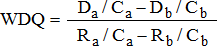
In terms of interpretation, a WDQ value of zero suggests that the crime rate in the catchment area changed at the same rate as it did in the control area. Positive values suggest that the crime rate in the catchment area decreased at a rate that exceeded changes observed in the control area and, negative values suggest the opposite. The observed effect is expressed relative to the changes observed in the treatment area, so a value of one indicates that the observed change in the catchment area was of the same magnitude as that observed in the treatment area. The WDQ can also be broken down into separate measures of scheme success and scheme displacement/ diffusion, like so:

Success Measure (WDQ denominator) = R_a/C_a – R_b/C_b

Catchment¹⁷ Displacement Measure (WDQ numerator) = D_a/C_a – D_b/C_b

Additionally, the overall impact of the project was estimated using the TNE or “total net effects” equation which is defined by the relationship:

TNE = [R_{b} C_{a} / C_{b}) - R_{a}] + [D_{b} (C_{a} / C_{b}) - D_{a}]

The TNE provides an estimate of the overall effect of an intervention on crime. That is, given the changes observed in the control area(s), and any changes in the catchment area, what is the difference in the volume of crimes observed in the treatment and catchment areas compared with what would have been expected in the absence of intervention? A positive number suggests that the intervention was effective overall whereas a negative number implies that it was not- and in fact, appeared to add to the crime problem.

The WDQ was initially formulated for the analysis of changes in crime rates rather than counts. Moreover, the formula described above is used to calculate only a point estimate. Here we describe a modified version of the equation and a simple method for estimating confidence intervals for the point estimate.

Considering the point estimate of the WDQ, crime rates have the advantage of standardizing the values used in the equation. This is particularly appealing where an equation considers differences in differences, as is essentially the case with the WDQ. Where rates are replaced with counts in such an equation, there may be a scaling issue if the areas considered in the equations differ considerably in terms of the volume of crime experienced. Such differences are likely to arise if geographic locations compared differ in terms of their respective sizes (i.e. km²). Where rates cannot be used, one way of accounting for such differences is to work with logarithms rather than raw counts. This is the approach adopted here:

WDQ = \frac{L o g_{e} (D_{a} / C_{a}) - L o g_{e} (D_{b} / C_{b})}{L o g_{e} (R_{a} / C_{a}) - L o g_{e} (R_{b} / C_{b})}

As with the odds ratio estimates presented in the previous section, while a point estimate for the WDQ is useful it will be subject to error and it would be beneficial to estimate how large that error is likely to be. Doing so would provide an indication of the range of values within which the true value is likely to be found. As the sampling distribution for the WDQ is unknown, it would be less than ideal to specify a formula that relies on parametric assumptions to estimate the standard error. An alternative approach is to compute confidence intervals using non-parametric bootstrapping which does not rely on a-priori assumptions about a statistic's distribution (e.g. Moore & McCabe, 2006). In short, bootstrapping uses Monte Carlo resampling to estimate a sampling distribution using data for a single sample. We will not elaborate further on the method here as the detail would be rather technical. However, it is important to say that as with the confidence intervals produced for the odds ratios, the approach is not without criticism and hence the reader is urged to treat confidence intervals as indicators of the range within which the true value of the WDQ is likely to lie, rather than precise estimates.

4. Findings

4.1 Selection of studies

Table 1 summarises the results of the systematic search. The electronic database search identified over 2,500 studies (see Appendix B for more details). The titles and abstracts of these studies were then reviewed and any studies that were obviously not evaluations of focused policing interventions, obviously lacked a quantitative measure of crime and disorder or were book reviews were then removed. Articles reporting on systematic reviews or meta-analyses were also excluded from the short list at this point. This left a total of 103 studies. The full text of these 103 studies was then reviewed to determine whether they met all the relevant selection criteria when examined in detail. This process determined that 38 of these met the criteria, and the remaining 65 did not. As Table 1 demonstrates, a further 41 studies meeting the criteria were identified from the other elements of the systematic search (from the review of bibliographies, professional organisations, forward searches hand searches and recommendations from experts).

Table 1

Systematic search results

	Database	Bibliography	Forward	Organisation websites	Policing agencies	Hand	Other	Total
Study meets criteria	38	24	0	5	0	6	6	79
Study does not meet criteria	65	59	32	14	5	12	14	201
Not known if criteria met	0	5	0	1	0	0	3	9
TOTAL	103	88	32	20	5	18	23	289

Of the 79 studies that met the criteria, in 27 cases the study presented findings that were reported elsewhere, and were therefore removed to avoid duplication. In a further 8 cases, the study met the criteria but the figures could not be sourced (e.g. figures no longer available or author untraceable). The final 44 studies, that are used and described in the pages which follow, are listed in full in the eligible study reference list at the end of this report. A further list is given of the excluded studies that seemed eligible from the title or abstract but were excluded when examined in detail. This is a full list of all 201 studies marked as not meeting the criteria in Table 1. Appendix C displays a flow chart which summarises the entire search process and gives details of the various uses of the studies meeting the criteria.

4.2 Characteristics of studies

The 44 coded studies differed in their methodological approach. To account for the varying levels of methodological rigor, studies were grouped according to a hierarchy of evidence (see Table 2). The majority (57%) had simple pre and post assessments, and the remainder pre and post- with at least one control area. A minority (9%) used random assignment to minimize bias. Also, in the minority were studies which use a separate catchment for the control area (14% of studies). Note that all the studies included in this review had separate pre and post counts for at least one displacement/diffusion catchment area.

Table 2

Hierarchy of Evidence

Design	Treatment area	Control area	Treatment catchment	Control catchment	N(%)
RCT	X	X	X	X	4(9%)
RCT	X	X	X		1(2%)
Quasi- Experimental	X	X	X	X	2(5%)
Quasi- Experimental	X	X	X		12(27%)
Quasi- Experimental	X		X		25(57%)

As expected, a range of different data and methods were used across the different primary studies. In some cases multiple treatment, control and or/catchment areas were used within one primary study and effect sizes were calculated for a number of different combinations of these areas. Furthermore, some studies looked at effects for a number of different types of crime data (e.g. CFS, arrests and recorded crime) and crime types. Finally the methods used varied across studies; some used time series data; others crime counts and/or crime incident rates. A number of different methods were used for calculating effect sizes and statistical significance. These are characterized more extensively in the narrative section below.

Table 3 lists some descriptive statistics for the studies. Many of the studies reported interventions that had taken place in the US (68%) or UK (23%). A range of different environments were covered by the interventions. Many covered purely residential environments (52%) or multiple types of environment (20%). 4 studies were undertaken in mixed areas containing both residential and retail; two in retail areas exclusively. The most common type of data that was used was Recorded Crime (35 studies); Calls for Service data was used in 7 studies; 4 used arrest data and 1 used data from primary observation. The studies also varied in terms of the extent of physical area that was covered by the initiative; 24 studies covered ‘large’ areas, 9 medium and 11 small¹⁸. Finally, the studies covered a range of different intervention types; most common was Problem-Orientated Policing (27%), Police Crackdowns (23%), Police Patrols (16%), Community orientated policing (11%) and Hotspot policing (9%).

Table 3

Descriptive Statistics of Eligible Studies

Characteristic	Category	N
Size	Large	24
	Medium	9
	Small	11
Country	US	30
	UK	10
	Sweden	1
	Australia	3
Environment	Multiple	9
	Various	4
	Retail	2
	Educational	1
	Recreational	1
	Residential	23
	Residential and retail	4
Intervention Type	POP	12
	Patrols	7
	Hotspots Policing	4
	Police Crackdown	10
	Intelligence-Led Policing	2
	Community-Orientated Policing	5
	Broken Windows	2
	Civil Abatement	1
	Police-Led Environmental	1
Data Type	Recorded Crime (RC)	33
	Calls For Service (CFS)	5
	RC and CFS	1
	CFS/Arrests	1
	RC/Arrests	1
	Arrests	2
	Primary Observations	1

4.3 Narrative review of displacement and diffusion from geographically focused policing initiatives

Appendix D summarizes the 44 studies included within this review. In each case a description is given of the intervention itself, the context in which it was implemented and the author's findings in terms of both the success of the treatment and the effect the treatment had in terms of spatial displacement. These are organized into three sections; those that were included in the meta-analysis and the proportional change analysis¹⁹; those that were not in the meta-analysis but were in the proportional change analysis and those that were not in either; but in which findings were reported by the author.

The following section gives a brief overview of the findings that were reported by the authors. This is an unusual addition to a systematic review where the focus is traditionally on the findings of the meta-analysis. We include this summary as a consequence of the unusual nature of this particular review. In essence, we are attempting to summarise two effect sizes- that of the treatment itself and that of any consequent diffusion or displacement. Methods used to investigate these two effects vary substantially across studies, hence we feel it would be incomplete to proceed without passing comment on these variations. We refer readers with less interest in this directly to section 4.4 which presents findings of the meta-analysis.

Summary of the Narrative review

Appendix D demonstrates that a broad range of different types of intervention, implemented in different contexts, have been evaluated across studies. It is also clear that he authors' findings vary across studies. In summarizing the findings it is important to provide some sense of the extent to which authors reported spatial diffusion and/or displacement as a result of intervention. As has been demonstrated elsewhere (e.g. Petticrew and Roberts, 2006), as method of synthesizing evidence, simple vote counting has many dangers. However, with this warning in mind it is valuable to provide an overview of the findings of all 44 studies, as only a subset of those (n=16) are used in the main meta-analysis reported below. Hence, for descriptive purposes only we include such a narrative summary here. This reveals differences between study authors' findings with respect to the likelihood of them reporting that they observed displacement or a diffusion of benefit. We see that 55% of the studies reported finding no spatial displacement; compared to 39% who did find evidence. For diffusion of benefit, this was found in 43% of studies and not in 5%. For the remaining 7% (displacement) and 52% (diffusion) of studies respectively, outcomes are unknown mainly due to the fact that they were not explicitly examined by the study authors. This indicates that there remains a bias in the literature whereby evaluators appear more likely to look for displacement rather than diffusion of benefit.

For completeness, Table 4 gives details of authors' statistical testing of the significance of displacement or diffusion of benefit. This table only includes studies for which a test has been used- and not where assessments have been made on the basis of descriptive statistics. Its purpose is to demonstrate the methods used by study authors. It is apparent from Table 4 that displacement and diffusion are explored using many different designs and statistics. There is no standard (or even particularly frequently used) method of hypothesis testing. The most common type of design tested group differences using ANOVAs or T-tests. The authors who have used t-tests (Smith 2001; Weisburd et al 2006; Wagers 2007; Segrave and Collins 2005 and Sherman and Rogan 1995) tend to calculate statistics for treatment, control and catchment areas separately, comparing monthly or weekly counts before or after the intervention. The same is true of those using ANOVAs or reporting F statistics (Priest and Carter 2002, Ratcliffe and Makkai (2004), Weisburd and Green (1995) and Farrell et al (1998). Very few modeled interaction effects or considered the treatment and control changes together. Interrupted time series designs were used in 4 of the studies (Katz et al 2001, Lawton et al 2005, Novak et al 1999 and Roman et al 2005). Katz et al modeled the treatment and catchment area effects separately; Lawton et al and Roman et al modeled the treatment, catchment and control areas separately; and Novak et al added a fourth model for a catchment control area. The time series modeling was done with varying degrees of sophistication regarding spatial lags and autocorrelation to account for temporal dependency in the data. Regression analysis was used in three studies (Braga and Bond 2008; Braga et al 1999 and Eck and Spelman (1987). The latter used monthly time point data in their analysis, whilst the others used pre and post data for multiple treatment, control and catchment areas. One study used correlation (Chenery et al 1997) and in this case the authors correlated rates in the treatment area with those in the adjacent divisions before and during the intervention. One study (McCabe 2009) used hierarchical linear modeling to enable simultaneous modeling of effects in distinct treatment areas.

Table 4

Authors' statistical testing of the significance of displacement or diffusion of benefit

Article	Authors Conclusion
Chenery, S., Holt, J. & Pease, K. (1997), Biting Back II: Reducing repeat victimization in Huddersfield. Crime Detection and Prevention Series, Paper 82, Home Office.	The monthly burglary rates for the action area were correlated with the rates for the adjacent divisions and for the police force area as a whole, both before and during the intervention. No significant negative correlations were found after the intervention had been implemented, which is indicative of a lack of spatial displacement. In fact, significant positive correlations were found during the initiative for one of the adjacent areas (r=0.67, p<.01) and for the force area (r=0.68, p<.01), which could be taken to indicate a diffusion of benefit. The authors, however, stated they were not making such a claim, as other factors could be responsible for the burglary reductions observed in non-action areas (see p. 38).
Eck, J. & Spelman, W. (1987), Problem-Solving: Problem oriented policing in Newport News. Police Executive Research Forum.	Ordinary least square (OLS) regression analyses were performed using residential burglary data for the targeted apartment complex and, separately, for the surrounding area (1 mile radius). In both cases, 37 data points were available pre-intervention and 17 months post-intervention. Treatment area effects: Results showed that the best fit was obtained for an abrupt, permanent effect, which showed burglary rates went down by 34.7% (b=-.347, SE=0.135 - all results given are for logged data). Catchment area effects: No significant changes in burglary rates were detected (b=0.026, SE=0.111), meaning no evidence of displacement or diffusion of benefit could be found.
Katz, C. M., Webb, V. J. & Schaefer, D. R. (2001). Assessment of the impact of quality-of-life policing on crime and disorder. Justice Quarterly, 18 (4), 825-876.	Two forms of an abrupt interrupted time series model were used to measure the effect of the intervention (implemented in two phases, with an inter-intervention period in between). Treatment area effects: For a zero-order transfer function with abrupt, permanent impact of the 10 CFS types examined, post-intervention the intervention was only found to effect significant reductions in the action areas for public morals (b=-0.16, SE=0.04), while significant increases were observed for physical disorder (b=0.24, SE=0.11). For a first order transfer function with abrupt, temporary effect model, no significant reductions were observed in the action areas for any of the crime types examined, but significant increases were detected for drugs (b=5.18, SE=0.90) and disorderly conduct (b=3.49, SE=1.57). Similar results are reported when the two intervention time periods (instead of the post-intervention period) were compared to the baseline. Catchment area effect: The type of model used is unclear, but reported results for the post-intervention period indicated CFS had significantly increased in surrounding areas for a number of crime categories including traffic (intervention parameter b=0.48, SE=0.10), physical disorder (b=0.15, SE=0.04), assistance (b=0.09, SE=0.03) and drug crime (b=0,06, SE=0.03). For the two intervention periods, only physical disorder (b=0.15, SE=0.05 - in phase one) and traffic (b=0.30, SE=0.13 - in phase two) showed significant increases.
Lawton, B.A., Taylor, R.B. & Luongo, A.J. (2005). Police Officers on Drug Corners in Philadelphia, Drug Crime, and Violent Crime: Intended, Diffusion, and Displacement Impacts. Justice Quarterly, 22 (4), 427-451.	Time series analyses were performed separately for the action, control and catchment areas, and also for violent and drug crimes. In each case, the crime counts per week were considered, with 121 weeks considered before and 18 weeks after the intervention had been implemented. Treatment area effects: An ARIMA (1,0,1) model provided the best fit and its results showed violent crime had significantly reduced (b=-.99, SE=0.26, p<.001). Significant reductions were also found for drug crime, both when using an ARIMA (1,0,1) model (b=-2.96, SE=0.59, p<.001) and an ARIMA (1,0,0) model (b=-2.93, SE=0.56, p<.001) - the authors argued that neither model was superior, so both sets of findings were reported. Control and catchment area effects: For violent crime, the ARIMA (1,0,1) model showed no significant effects for the control area (b=-0.64, SE=0.41, ns) but a significant reduction for the catchment area (b=-0.363, SE=0.15, p<.05), providing evidence for diffusion of benefit. For drug crime, different pictures emerge when using alternative models. The ARIMA (1,0,1) model is indicative of displacement, with no significant effects reported for the control area (b=0.54, SE=0.46, ns) but significant increases in the catchment area (b=0.71, SE=0.16, p<.001). On the other hand, the ARIMA (1,0,0) model indicated that, while no significant effects could be detected for the control area (b=-0.30, SE=0.42, ns), drug crime significantly decreased in the catchment area (b=-0.89, SE=0.41, p<.05), which is indicative of diffusion of benefit.
McCabe, James E. (2009). The Narcotics Initiative: An Examination of the NYPD Approach to Drug Enforcement, 1995-2001. Criminal Justice Policy Review, 20, 170-187.	The initiative was implemented in two phases, each in different police precincts, and its effectiveness was measured using hierarchical linear modelling (which allows for the simultaneous examination of individual precincts' time series). Treatment area effects: Three output measures were examined, namely the rates for Part I recorded crime, controlled substance arrests and marijuana arrests. Significant reductions in Part I crime rates were observed during phase one (b=-28.06, SE=10.40, t=-2.70, p<05) but not during phase two of the intervention (b=2.55, SE=8.03, t=0.32, ns). No significant changes in the rate of controlled substance arrests were reported, either during phase one (b=-5.85, SE=3.93, t=-1.49, ns) nor phase two (b=2.49, SE=3.59, t=0.69, ns). Significant reductions in the marijuana arrest rates were observed for phase one (b=23.56, SE=5.67, t=4.16, p<01) but not for phase two (b=13.01, SE=6.68, t=1.95, ns). Catchment area effects: For Part I crime, no changes were observed during phase one (b=-5.09, SE=5.89, t=-0.86, ns) but significant increases were apparent during phase two (b=18.70, SE=5.82, t=3.21, p<.01). No significant changes in the number of controlled substance arrests in the catchment areas were reported, either during phase one (b=4.55, SE=4.52, t=1.01, ns) nor phase two (b=-5.30, SE=4.32, t=-1.23, ns). The same pattern was observed in relation to marijuana arrest rates, with no significant effects detected either during phase one (b=2.65, SE=2.49, t=1.06, ns) nor phase two (b=1.97, SE=2.89, t=0.68, ns).
Novak, K.J. Hartman, J.L., Holsinger, A.M. & Turner, M.G. (1999). The Effects of Aggressive Policing of Disorder on Serious Crime, Policing: An International Journal of Police Strategies & Management, 22 (2), 171-190.	Interrupted time series analyses were performed for each of four areas (i.e. action, control, buffer around action and buffer around control) and two crime types (i.e. robbery and aggravated burglary). Treatment area effects: No significant effects were reported for either crime type. This was the case regardless of the model employed, namely: zero-order transfer function for abrupt, permanent effects; first-order transfer function for gradual, permanent effects; and first order transfer (pulse) function to a differenced series for abrupt, temporary effects (due to the lack of significant effects and the large number of coefficients, these are not reported here; see Table II on p. 184 in original paper). Control and catchment area effects: Again, no significant effects were observed, regardless of crime type, area type or time series model. The authors stated the patterns observed may be due to a lack of statistical power, resulting from low crime counts.
Priest, T. B. & Brown Carter, D. (2002). Community-oriented policing: Assessing a police saturation operation (from policing and community partnerships, P 111-124, 2000, dennis J. stevens, ed., – see NCJ-194083). Retrieved from http://www.policetrainings	Weekly crime counts were compared before and after the intervention (9 weeks in each period), in relation to all crime, violence, property crime and other crime. Treatment area effects: Although the mean weekly counts went down for all crime categories examined, these differences were not significant (all crime down from 16.89 to 15.00 incidents per week, F=0.801; violence down 5.22 to 4.55, F=0.401; property down 8.33 to 7.22, F=0.557; other down 3.33 to 3.22, F=0.015). Catchment area effects: No significant effects were found in the catchment areas either but the trends varied across crime types as follows: all crime increased from 5.00 to 5.22 incidents per week (F=0.028); violent crime decreased from 2.33 to 1.56 (F=0.699); property crime went up from 1.77 to 2.44 (F=1.469); and other crime also increased from 1.00 to 1.22 incidents per week (F=0.113).
Ratcliffe, J. & T. Makkai. (2004). Diffusion of Benefits: Evaluating a Policing Operation. Trends & Issues in Crime and Criminal Justice, 278, Australian Institute of Criminology, Canberra.	One-way ANOVA tests were used to compare weekly crime counts were compared before (113 weeks) and after (88) the intervention, in relation to burglary and car crime. Treatment area effects: Significant reductions were reported both in relation to burglary (down from 144 to 114 crimes per week, F=47.45, p<.01) and car crime (down from 93 to 82 crimes per week, F=13.82, p<.01). Catchment area effects: Significant reductions were reported both in relation to burglary (down from 54 to 49 crimes per week, F=9.56, p<.01) and car crime (down from 37 to 33 crimes per week, Welch=8.10, p<.05), which indicates the benefits of the intervention were diffused to neighbouring areas.
Roman, C., Cahill, M., Coggeshall, M., Lagerson, E. & Courtney, S. (2005). Weed and seed initiative and crime displacement in south Florida: An examination of spatial displacement associated with crime control initiatives and the redevelopment of public housing	Time series models were used to measure the effect of the intervention on the monthly crime counts for violence and drug-related incidents, separately for the action, control and catchment areas. All time series were differenced on lag 1 to remove non-seasonal trends and, in most cases, also differenced on lag 12 to remove the seasonal trend. Adjustments were made for varying month lengths and log transformations were also applied. The pre- and post-intervention periods lasted 48 months each (pre 1995-1998; post 1999-2003). Treatment area effects: No significant effects were found for violent crime (best fit step function, b=0.92, SE=0.04, ns), whereas drug-related incidents increased following the intervention (3-month decay function, b=2.21, SE=0.42, p<.05). Control and catchment area effects: For violent crime, significant reductions were observed both in the control (step function, b=0.88, SE=0.05, p<.05) and the catchment area (step function, b=0.72, 0.07, p<.05). For drug-related crime, no significant changes were observed for either the control (step function, b=1.66, SE=0.47, ns) nor the catchment area (pulse function, b=1.31, SE=0.45, ns).
Smith, M. R. (2001). Police-led crackdowns and cleanups: An evaluation of a crime control initiative in Richmond, Virginia. Crime and Delinquency, 47(1), 60-83.	Weekly crime counts were compare pre- (26 weeks) and post-intervention (4) for four areas (one target, three catchment) and three crime types (total Part I offences, violent crime and property crime). Treatment area effects: Significant reductions were observed for total Part I offences (down from 2.35 crimes per week to 0.25, t=-2.61, p<.05) and violent crime (down from 0.58 to 0.00, t=-4.186, p<.01) but not for property crime (down from 1.77 to 0.25, t=-1.85, ns). Catchment area effects: In the first catchment area, no significant effects were found for either total Part I offences (down from 1.27 to 1.00, t=-0.37, ns), violent crime (down from 0.54 to 0.25, t=-0.45, ns) nor property crime (down from 0.73 to 0.50, t=-0.51, ns). In the second catchment area, significant reductions were observed for total Part I crime offences (down from 5.42 to 2.25, t=2.03, p<.05) and violent crime (down from 1.15 to 0.00, t=5.25, p<.01) but not for property crime (down from 4.27 to 2.25, t=-1.54, ns). In the third catchment area, no significant changes were observed for either crime type: total Part I offences (down from 4.04 to 2.25, t=-1.62, ns); violent crime (up from 0.73 to 0.75, t=0.04, ns); and property crime (down from 3.30 to 1.30, t=-1.93, ns).
Weisburd, D., & Green, L. (1995). Policing drug hot spots: The Jersey City Drug Market Analysis experiment. Justice Quarterly, 12(4), 711-742.	Mixed model ANOVA tests were used to examine the interaction between group (treatment vs. control) and block (very high arrest and call activity vs. high vs. medium vs. low activity). The dependent variable was the mean change in the number of calls for service for eight different crime categories: violence; property; disorder (also broken down into nuisance, suspicious persons, public morals and assistance); and narcotics. A unique sums of squares methods was employed, with 15 degrees of freedom for explained variance and 40 for residual. Treatment area effects: Significant effects were found for nuisance (Treatment=9.14, Control=25.39; p=.007), suspicious persons (T=-0.11, C=5.96; p=.001), and public morals (T=-2.14, C=0.89; p=.032). Catchment area effects: Significant differences between the groups were found for public morals (Buffer around T=-11.32, Buffer around C=0.68; p=.001) and narcotics (Buffer around T=-5.25, Buffer around C=18.14; p=.015).
Weisburd, D., Wyckoff, L.A., Ready, J., Eck, J.E., Hinkle, J.C. & Gajewski, F. (2006). Does crime just move around the corner? A controlled study of spatial displacement and diffusion of crime control benefits. Criminology: An Interdisciplinary Journal, 4	The number of prostitution-, drug- and disorder-related events per observation were compared pre- (30 days), during (182 for prostitution, 212 for drugs/disorder) and post-intervention (61 for prostitution, 31 for drugs/disorder). Treatment area effects: For prostitution, significant reductions were observed both during (i.e. as compared to the pre-intervention period; down from 2.96 events per observation to 1.04; t=-3.20, p<.01 -1 adjusted for citywide trends in emergency calls for service for disorder) and post-intervention (1.17 events per observation; t=-3.59, p<.001). For drugs, significant reductions were observed both during (down from 1.30 to 0.40; t=-2.39, p<.05) and post-intervention (0.14 events per observation; t=-3.40. p<.001). For disorder, significant reductions were observed both during (down from 4.10 to 0.91; t=-3.86, p<.001) and post-intervention (0.75 events per observation; t=-4.76, p<.001). Catchment area effects: There were two catchment areas: one covering the street block surrounding the action areas; the other surrounding the first catchment area, also one block wide. For prostitution, significant reductions were observed during the intervention in the first catchment area (down from 1.01 to 0.26, t=-2.18, p<.05) but not in the second (down from 0.37 to 0.11, t=-1.64, ns); however, significant reductions were observed in both catchment areas when comparing the post- and the pre-intervention periods (catchment area 1 had 0.24 events per observation, t=-3.01, p<.01; catchment area 2 had 0.07, t= -2.70, p<.01). For drugs, no significant changes were observed, either during (catchment area 1 down from 0.18 to 0.06, t=-0.60, ns; catchment area 2 down from 0.31 to 0.04, t= -1.34, ns) nor after the intervention (catchment area 1 had 0.06 events per observation, t=-0.53, ns; catchment area 2 had 0.01, t= -1.50, ns). For disorder, significant changes were observed, both during (catchment area 1 down from 2.54 to 0.53, t=-2.88, p<.01; catchment area 2 down from 1.33 to 0.36, t= -3.17, p<.01) and after the intervention (catchment area 1 had 0.39 events per observation, t=-3.69, p<.001; catchment area 2 had 0.21, t= -4.55, p<.001).
Braga, A. A. & Bond, B. J. (2008), Policing crime and disorder hot spots: A randomized controlled trial. Criminology: An Interdisciplinary Journal, 46 (3), 577-607.	Poisson regression analyses were performed to measure the effect of the intervention on both action and catchment areas, for six types of calls for service (assault, robbery, burglary/breaking and entering, larceny/theft, disorder/nuisance and total calls). Treatment area effects: Significant reductions were observed for assault (b=-4.418, SE=0.102, Z=-4.10, p<.01), robbery (b=-0.541, SE=0.254, Z=-2.13, p<.05), burglary/breaking and entering (b=-0.438, SE=0.118, Z=-3.69, p<.01) and total calls (b=-0.220, SE=0.084, Z=-2.60, p<.01) but not for larceny/theft (b=-0.113, SE=0.076, Z=-1.48, p=.139) nor disorder/nuisance (b=-0.169, SE=0.106, Z=-1.75, p=0.081). Catchment area effects: No significant effects were found for any of the call types examined (Z values ranged from 0.46 to 1.50; see Table 4, p. 598, in original paper for all the test statistics).
Braga, A. A., Weisburd, D. L., Waring, E. J., Mazerolle, L. G., Spelman, W. & Gajewski, F. (1999), Problem-oriented policing in violent crime places: A randomized controlled experiment. Criminology, 37 (3), 541-580.	Regression analyses were performed to measure the effect of the intervention on both action and two-block catchment areas, for five types of calls for service (CFS; robbery, street fight, property, disorder/nuisance and narcotics) and five (equivalent) types of recorded crime or arrests (robbery, non-domestic assault, property, disorder/vandalism and narcotics arrests). Treatment area effects: Significant reductions were observed for street fight calls (b=-0.599, X²=5.793, p<.05), property calls (b=-0.196, X²=7.150, p<.01), narcotics calls (b=-0.258, X²=8.694, p<.01), recorded robbery (b=-0.631, X²=4.607, p<.05) and recorded property crimes (b=-0.519, X²=25.591, p<.001; see Table 4, p. 563, in original paper for all the test statistics). Significant reductions were also found when all criminal incidents and all calls for services were considered as aggregated data sets (criminal incidents b=-.386, X²=39.976, p<.01; CFS b=-0.151, X²=18.289, p<.001; see Table 3, p. 562). Catchment area effects: Significant reductions were observed for disorder/nuisance calls (b=-0.112, X²=4.547, p<.05), recorded assault (this includes domestic incidents though; b=-0.219, X²=5.651, p<.05) and also for all aggregated calls (b=-0.086, X²=11.276, p<.001). A significant increase in recorded property crime was also observed (b=0.181, X²=8.335, p<.01; see Table 7, p. 568, for more test statistics).
Farrell, G., Chenery, S. & Pease K. (1998), Consolidating police crackdowns: Findings from an anti-burglary project. Police Research Series Paper 113, London, UK.	One-way ANOVA tests were used to compare the monthly burglary counts between the action, control and catchment areas, at three different time points (i.e. pre-, during and post-intervention). Significant differences could be found among the three areas, both before (Action=44.9, Catchment=41.4, Control=21.0; F=35.7, p<.001; Newman-Keuls - all pairwise differences significant except for Action vs. Catchment) and during the intervention (Action=48.7, Catchment=35.1, Control=21.1; F=24.5, p<.001; Newman-Keuls - all pairwise differences significant). After the intervention, however, no significant differences could be found among the three areas (Action=18.5, Catchment=20.6, Control=17.4; F=0.9, ns; Newman-Keuls - all pairwise differences non-significant).
Segrave, Marie & Collins, Lisa (2005), Evaluation of a suburban crime prevention team, Technical and background paper series, 14, Australian Institute of Criminology, Canberra.	Weekly crime rates were compared before (26 weeks) and after (26) the intervention in relation to violence, property crime and disorder. In each case, the action area was compared to a control area as well as three contiguous areas. Treatment area effects: No significant effects were found for either crime type (violence down from 0.9 to 0.6 crimes per week, F=1.39, p=0.24; property crime up from 7.7 to 9.8, F=3.12, p=0.08; disorder down from 2.8 to 2.4, F=0.80, p=0.38). Control and catchment area effects: No significant effects were found for the control area in relation to either crime type (violence down from 1.1 to 0.8 crimes per week, F=1.06, p=0.31; property crime up from 8.1 to 9.4, F=1.16, p=0.29; disorder up from 2.9 to 3.3, F=0.48, p=0.49). For violence, a marginally significant increase was observed in the second catchment area (going from 0.8 to 1.5 crimes per week, F=3.98, p=0.05) with no significant differences found for either the first (down from 0.6 to 0.4, F=0.74, p=0.39) nor the third catchment area (down from 1.3 to 1.2, F=0.07, p=0.79). In relation to property crime, a significant increase was observed in the third catchment area (going from 7.8 to 12.3 crimes per week, F=5.77, p<.05) but not in the first (down from 7.3 to 5.6, F=1.63, p=0.21) nor the second catchment area (up from 13.8 to 16.3, F=1.74, p=0.19). For disorder, a significant increase was observed in the second catchment area (going from 5.1 to 7.0 crimes per week, F=4.84, p<.05) with no significant differences found for either the first (down from 2.4 to 1.5, F=3.03, p=0.09) nor the third catchment area (up from 3.2 to 4.9, F=2.20, p=0.14).
Sherman, L.W. & Rogan, D.P. (1995). Effects of Gun Seizures on Gun Violence: Hot Spots Patrol in Kansas City. Justice Quarterly, 12, p. 673.	Both t test and time series analyses were performed to measure the impact of the initiative on gun crimes. Treatment area effects: Crime counts significantly decreased from 169 in the 29 weeks prior to the intervention to 86 in the 29-week post-intervention period (t=-3.296, p<.01). Time series analyses revealed similar results (b=-2.558, SE=0.613, p<.05). Control and catchment area effects: The impact of the intervention on the control area was non-significant (crime count up from 184 to 192, t=0.279, p=0.781; b=-0.751, SE=0.080, ns). No significant differences were observed for any of the seven contiguous police beats when t tests were used (all seven areas aggregated contained 764 crimes before and 816 crimes after the intervention; t=0.62, p=0.537; individual comparisons had p values ranging from 0.143 to 0.869). Time series analyses indicated that no significant effects could be detected when all seven beats were aggregated (b=-2.577, SE=1.945, ns) although, when disaggregated, significant reductions were observed for two of the beats (beat 141 b=-0.981, SE=0.479, p<.05; beat 143 b=-0.692, SE=0.353, p<.05).
Wagers, M. (2007), Broken windows policing: The LAPD experience, Ph.D. diss., Rutgers The State University of New Jersey - Newark.	Mean monthly count of Part I crimes were compared one year before and one year after the intervention, separately for the action and a buffer area. Treatment area effects: A significant decrease was observed (from 158.08 to 116.17 crimes per month, t(22)=6.91, p<.001). Catchment area effects: Although the mean monthly crime count decreased (from 118.08 to 103.83), this difference failed to achieve significance (t(22)=1.55, p=0.135).

Theoretical centrality of displacement/diffusion

Appendix E provides an assessment of the degree to which study authors examined the issue of displacement or diffusion. For each study, we list whether displacement was examined centrally, peripherally, briefly or from a post-hoc perspective by each set of authors. We also indicate whether the research was informed by prior research or theory and provide details of the rationale given for the study and the examination of displacement. The appendix also provides details about the intervention implemented, the study context and design, and findings regarding displacement and/or diffusion for cross-referencing purposes.

It is apparent from Appendix E that in many cases (59%) -but by no means all of them - the research was informed by prior research or theory concerning the possibility that crime might be displaced. There was a fair degree of variation in terms of how centrally the issue of displacement was examined; in 18 (41%) of cases it was centrally examined; in 10 cases there was a brief discussion; it was examined peripherally in 7 cases and undertaken as post-hoc analysis in a further 7 studies. This demonstrates that is it not possible to assume that authors have given the same weight to the issue of displacement in their research.

Cross-tabulations of the data revealed that there were no real differences in the extent to which displacement or diffusion was centrally addressed for those studies in which areas were assigned to treatment and control groups using a random allocation strategy and those that employed a quasi-experimental design. Similarly, those studies for which data were collected for treatment, control, catchment and catchment control areas examined displacement and diffusion of benefits with roughly the same likelihood as those for which data were not collected for catchment control areas.

4.4 Meta-analysis

4.4.1 Summary of the data used

Across the 44 studies, the most consistently reported findings were descriptive statistics that contrasted the counts of crime pre- and post- intervention for (at least) one treatment area, one control area, and one catchment area that surrounded the treatment area. Crime counts for the periods before and after intervention were available for treatment, catchment and control areas for 16 studies. However, the evaluation design employed varied across studies. Table 5 summarises this data. For most (N=11), only one control area was used for the treatment and catchment areas. However, for a small number of studies (N=5), independent control areas were identified for both the treatment and catchment areas. In some studies, data were collected for more than one catchment area for each treatment area (N=4). For others, data were collected for the periods before, during and after intervention. For some studies (N=5), areas were allocated to treatment and control conditions randomly, but for the majority they were not (N=11). Finally, some studies gave counts for multiple crime types, while others only examined a single category of offense (N=12). One consequence of these methodological differences is that it was possible to calculate more than one odds ratio for some of the studies.

Table 5

Summary of the evaluation designs of the studies in the meta-analysis

	RCT	Periods	Control areas	Catchment controls?	Catchment area(s)	Crime type (and Source)
Allatt (1984)	No	Before, during and after	One area selected	No	Two adjacent estates selected. One of private, one of public housing.	Burglary (RC)
Braga & Bond (2008)	Yes	Before, after	17 control areas (collapsed data available for analysis)	Yes	17 catchment areas (collapsed data available for analysis)	All crimes (CFS)
Braga et al (1999)	Yes	Before, after	12 control areas	Yes	12 catchment areas	All crimes (RC/CFS)
Cummings (2006)	No	Before, during	One area selected	No	Two catchment areas	Burglary (RC)
Ebsensen (1987)	No	Before, during	One area selected as control; one area as catchment control	Yes	One catchment area	All crime/ Index Crimes/Public Disorder (RC)
Farrell et al. (1998)	No	Before, during and after	One area selected	No	One catchment area	Burglary (recorded crime)
Grogger (2002)	No	Before, after	One area selected	No	One catchment area	Gang Violence (RC)
Higgens and Coldren (2000)	No	Before, after	One area selected	No	One catchment area	Narcotics (RC)
Mazerolle et al (2000)	Yes	Before, after	50 control addresses;; 43 residential, 7 commerical (collapsed data available for analysis)	Yes	50 catchment addresses; 43 residential, 7 commerical (collapsed data available for analysis)	Drug Crime (CFS). Separated by Commercial/residential addresses
McGarrell et al (2001)	No	Before, after	One area selected	No	One catchment area	Fire-arm Related Crime (RC)
Press (1971)	No	Before, after	One area selected	No	One catchment area	Multiple categories- 10 ‘inside’ crime types and 10 ‘outside’ crime types (RC)
Ratcliffe et al (2010)	Yes	Before and during	60 control areas (collapsed data available for analysis)	No	55 catchment areas (collapsed data available for analysis)	Violent crime
Segrave & Collins (2005)	No	Before and after	One area selected	No	Three catchment areas; different adjacent areas	Violent crime, property crime, disorder
Sherman & Rogan (1995)	No	Before and during	One area selected	No	Two catchment areas; contiguous police beats and the remainder of the police force area	Gun crime
Wagers (2007)	No	Before and after	One area selected	No	One catchment area	Part 1 crime (recorded crime)
Weisburd and Green (1995)	Yes	Before and after	28 control areas (collapsed data on disorder-public morals available for analysis)	Yes	28 catchment areas (collapsed data on disorder-public morals available for analysis)	Violence/Property/Disord er and drug crime (CFS)

For many studies, there was only one treatment, catchment and control area. In others (e.g. Braga and Bond, 2008) there were multiple treatment, catchment and control areas. In the case of the latter, data were nearly always unavailable for each individual area and so analyses were conducted in the aggregate.

4.4.2 Best and Worst-case scenarios

Figures 1 and 2 show the individual effect sizes and confidence intervals for the best-and worst-case scenarios for both the treatment and catchment areas for all 16 studies. Where there was only one observation for a particular study, this was used in both the best- and worst-case scenarios. Where there were multiple observations, for the best-case scenario, the observations used were those for which the point estimate of the treatment effect was most positive (i.e. in favour of a treatment effect). If there were multiple observations for which there was an equal treatment effect, the observation for which the most positive effect was observed for the catchment area was selected.

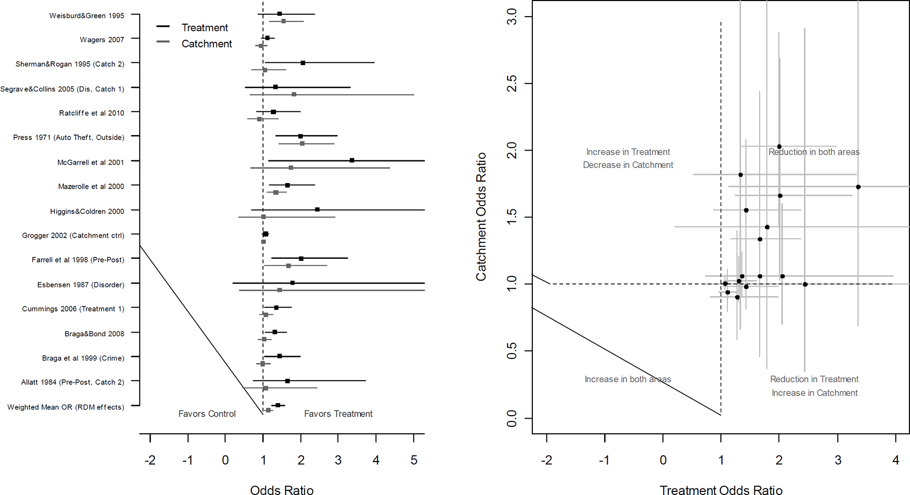
Individual effect size estimates and confidence intervals for the best case scenario across the 16 studies (Left panel), and a scatter plot showing the effect size estimates and confidence intervals for the treatment areas plotted against those for the catchment areas (Right panel)

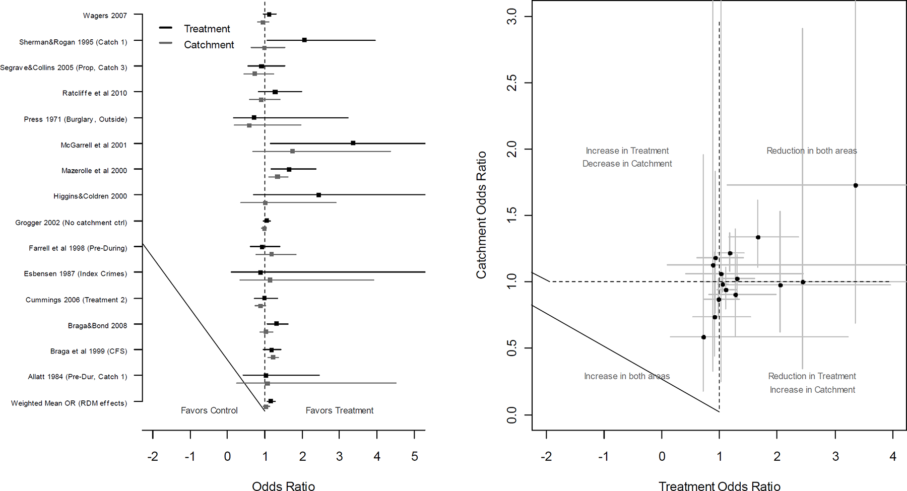
Individual effect size estimates and confidence intervals for the worst case scenario across the 15 studies (Left panel), and a scatter plot showing the effect size estimates and confidence intervals for the treatment areas plotted against those for the catchment areas (Right panel)

For some studies, data were available for catchment control areas as well as treatment control areas. When calculating the odds ratios for the catchment areas, we used the best available control area; that is, where there is a separate catchment control area we used that. Where there is not, we used the control area identified for the treatment area.

In Figure 1, the Forest plot (left panel) shows the point estimates and associated confidence intervals. Where the former is greater than one this indicates that the outcome favors treatment. Where it is less than one this indicates that crime increased in the treatment area at a rate that exceeded that observed in the control area (in relative terms). Considering the general trend, we computed the Q statistic (see Wilson and Lipsey, 2001) to determine if the variation in effect sizes indicated variation above and beyond that which would be expected for sampling error alone. For the treatment and catchments areas, the respective values of 34.8 (df=15) and 37.9 (df=15) were statistically significant at the p<0.05 level. Therefore, as might be anticipated there is significant heterogeneity in the effect sizes across studies. Hence, in line with the preferences expressed in Campbell Collaboration policy, to calculate the weighted mean effect, we used a random effects model. This is also more appropriate in a theoretical context, as our goal is to generalize to a hypothetical population of studies, which is only possible when account is taken of the between studies variance component (e.g. Hedges, 1992). For completeness, in all the analysis which follows, where the Q statistic is not significant, we also calculate the weighted mean effect using fixed effects, so comparisons can be made, but this was considered to be a secondary concern.

Overall, the weighted mean OR of 1.39 (CI: 1.22-1.59) suggests a positive significant effect at the treatment sites (p<0.05). In interpreting this finding the reader should recall that we included in this review only those studies for which data were available for treatment, catchment and control areas. Hence, other studies that examined changes in treatment and control areas alone are excluded from the analysis. Consequently, the reader should not interpret the effect size estimate for the treatment areas as representing the treatment effect for geographically focused police interventions in general, but just that for the subset of studies for which changes in catchment areas as well as the treatment and control areas were considered. For the catchment areas, the results are also positive and rather than suggesting that crime increased in the catchment areas, for the best case scenario the mean OR of 1.14 (CI: 1.03-1.14) indicates that it decreased overall (p<0.05).

Figure 2 shows the results for the worst case scenario. In this case, the Q statistic was not statistically significant for the treatment (Q=20.5, df=14, p>0.05) but was for the catchment (Q=26.9, df=14, p<0.05) areas and so both random effects and fixed effects model were conducted for the former and only a random effects model for the latter. The weighted mean (random effects) OR for the treatment areas of 1.15 (CI: 1.05-1.27) suggests a positive impact of intervention (p<0.05) ²⁰. For the catchment areas, the weighted mean OR of 1.04 (CI: 0.95-1.13) is in the same direction as that for the best-scenario but is non-significant. It is interesting to note that the difference between the weighted means for the best and worse-case scenarios is not large (ORs of 1.14 and 1.04 respectively).

4.4.3 Permutation Tests

As discussed above, one potential issue with presenting data for the best- and worst-case scenarios alone is that they may be overly sensitive to the presence of outliers. An alternative is to not only compute the best and worst case scenarios but all of those in between. Considering all studies, there are 69,120 possible permutations. Instead of computing every mean effect size we use a Monte Carlo simulation to sample 1000 unique mean effect size estimates from all possible permutations. For each (re)sample, we use a random effects model to compute the weighted mean effect sizes and confidence intervals as these provide a more conservative test of the hypotheses under investigation. Figure 3 shows the results of this analysis. The point estimates and confidence intervals at the top of the two Forest plots are a sample of the 1000 permutations, which are included for the purposes of illustration. The point estimates and confidence intervals at the bottom of the plot are the mean values computed across all permutations. Those shown in black represent the mean of the mean effect sizes and the mean of the upper and lower confidence intervals. Those shown in grey are the upper and lower 95% confidence intervals for the mean of the upper and lower confidence intervals²¹. Consistent with the results discussed above, the analysis suggests that relative to the control areas, there was a reduction in crime in both the treatment areas and catchment areas, although this was only significant for the treatment areas.

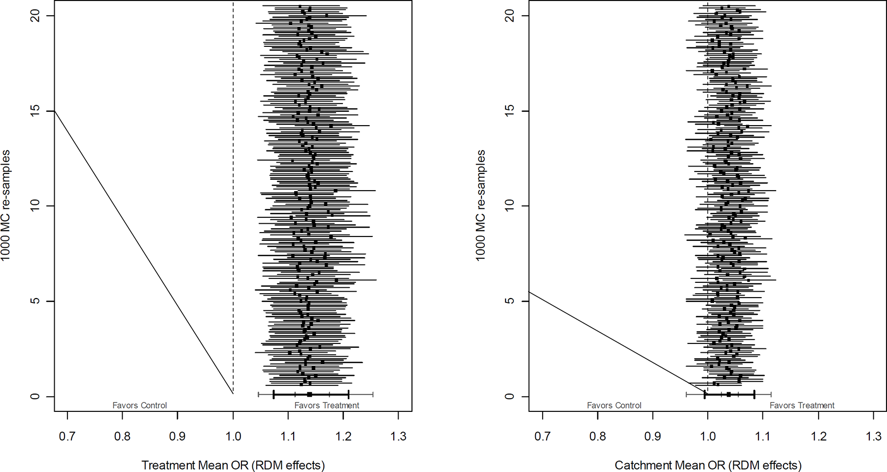
Weighted mean effect size estimates and confidence intervals for all studies for 200 of the 1000 Monte Carlo re-samples, and a summary of the distribution for the 1000 samples (Left panel: Treatment areas; Right panel: Catchment areas).

4.4.4 Assessing the effects of study design, intervention type and size of intervention.

Study design

In this section, analyses are presented for studies that may be meaningfully grouped together. In the first instance, we examine the results for those studies which employed a random allocation strategy to assign areas to treatment and control groups. Such studies minimize threats to internal validity (alternative explanations that might explain observed outcomes), assuming that the strategy of random allocation does generate comparable groups (and it should). In such cases, any changes observed in the treatment and catchment areas can be attributed to the effects of intervention with confidence (Campbell & Stanley, 1963). Thus, where a decrease in crime is observed in catchment areas (relative to the changes observed in the control areas) this may be interpreted as a diffusion of crime control benefits; this is the case even if little or no changes are observed in the treatment areas. Likewise, increases in crime in the catchment area which exceed those observed in the control area(s) may be interpreted as displacement; or at least as indicating that the treatment affected the spatial distribution of crime in a negative way (activity is not technically displaced if it continues to occur in one area and also increases in those contiguous, this would be a diffusion of offending activity).

In the case of quasi-experiments, causal inference will be weaker as other differences between groups (treatment, catchment and control) - particularly those that go unobserved by the investigators – may explain observed changes rather than the intervention evaluated. In such cases, an increase (decrease) in crime may indicate displacement (diffusion of crime control benefit) or it may be explained by other factors whose influences are not controlled for, or measured in the research design. For this reason, we analyze the data for the RCT and quasi-experimental studies separately.

For the RCT studies there were only two permutations of the data; one which included the recorded crime data analysed by Braga (1999) and one which included the calls for service data reported in the same study. Figure 4 shows the results for the former. For this analysis, the Q statistic was non-significant for the treatment areas (Q=1.51, df=4, p>0.75) but statistically significant for the catchment areas (Q=12.28, df=4, p<0.025)²². For the treatment areas, the weighted mean OR of 1.39 (CI: 1.20-1.60) suggests a positive effect of intervention. For the catchment areas, the weighted mean OR of 1.14 (CI: 0.97-1.35) suggests a non-significant diffusion of benefit.

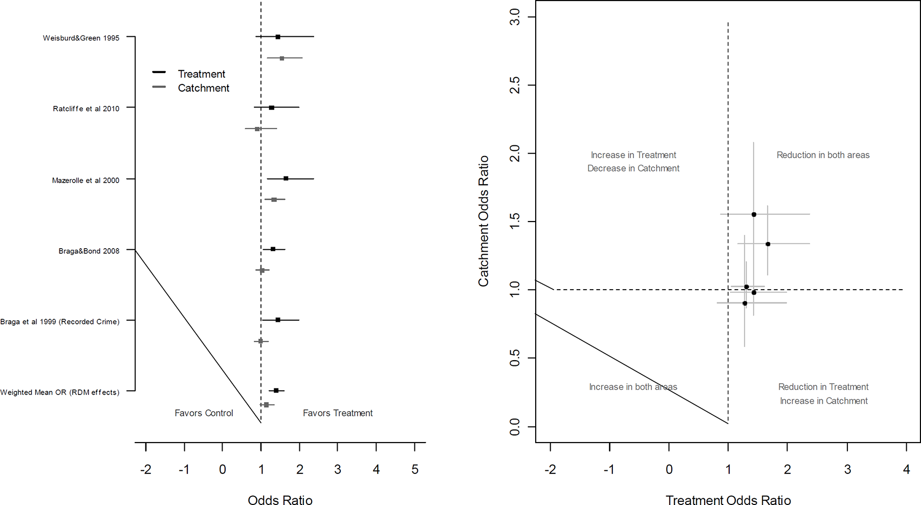
Individual effect size estimates and confidence intervals for the best case scenario across the 5 RCT studies (Left panel), and a scatter plot showing the effect size estimates and confidence intervals for the treatment areas plotted against those for the catchment areas (Right panel)

Figure 5 shows the second permutation of the data. In this case the Q statistics were less than the critical values for both the treatment (Q=2.81, df=3, p>0.25)²³ and catchment (Q=6.32, df=3, p>0.10), but for the reasons discussed above both fixed and random effects models were used to derive the weighted mean effects sizes - although we report only the latter here. For the treatment areas, the weighted mean effect size of 1.28 (CI: 1.13-1.46) suggested a positive effect of intervention for the studies considered. Likewise, for the catchment areas, the weighted mean effect size of 1.17 (CI: 1.04-1.29) suggested that, relative to the control areas, crime went down in the catchment areas.

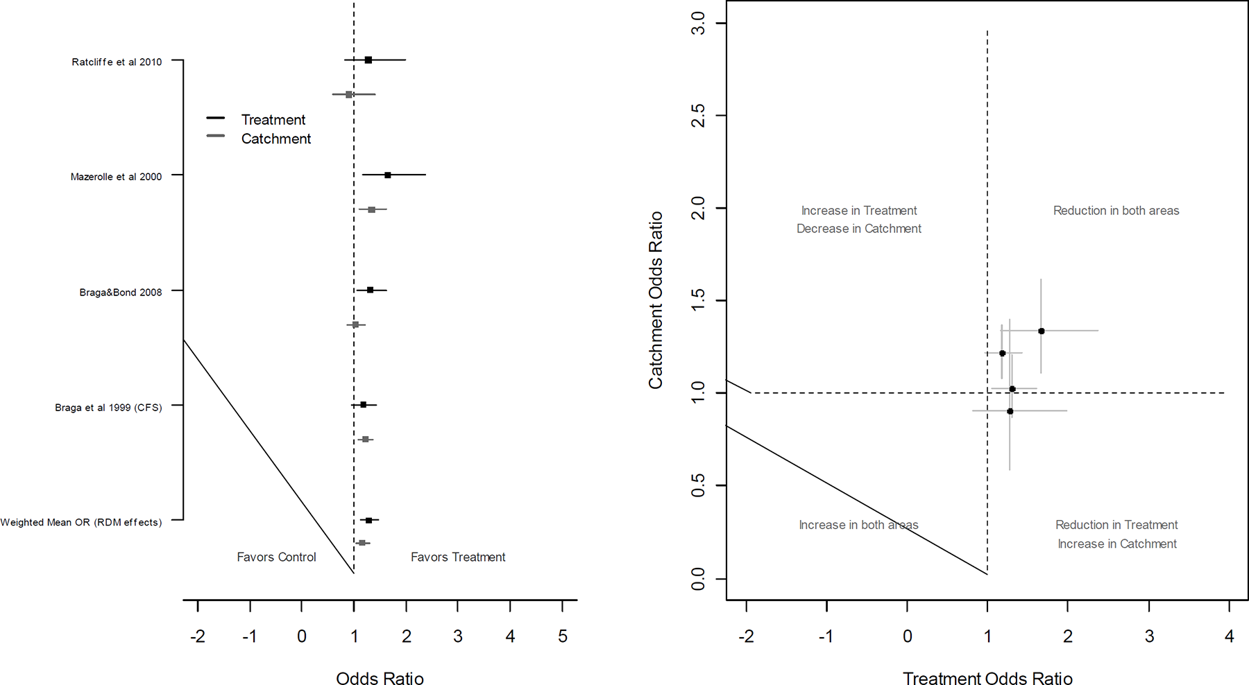
Individual effect size estimates and confidence intervals for the worst case scenario across the 4 RCT studies (Left panel), and a scatter plot showing the effect size estimates and confidence intervals for the treatment areas plotted against those for the catchment areas (Right panel)

Thus, for the studies with the highest level of methodological adequacy and for the two possible permutations, the trends are identical. Crime appears to have reduced significantly in the treatment areas. In the catchment areas, the conclusion is less clear but the worst case scenario suggests little or no change and the best case scenario indicates a diffusion of crime control benefit.

As discussed, for the quasi-experimental studies, threats to internal validity weaken the causal inferences that can be made. For this reason, it seems reasonable to apply stricter criteria when estimating the extent to which crime might have been displaced or benefits diffused when examining those studies which used quasi-experimental designs. One such criterion is that the search for displacement should be conditional on the demonstration of an intervention effect in the treatment area(s) (see Weisburd & Green, 1995; Bowers & Johnson, 2003). Of the quasi-experimental studies, significant reductions were estimated for five evaluations. For one of these, there were two observations and in the other there were five (in the first study data were reported for two catchment areas, in the other data were reported for different types of crime). Thus, there were four possible permutations of the data. For the sake of brevity, hereafter we do not report Q statistics and consistently report results that were derived using random effects models. Figure 6 shows the results for the best-case scenario. In this case, the weighted mean effect size of 1.66 (CI: 1.37-2.01) for the treatment areas and 1.39 (CI: 1.04-1.86) for the catchment areas suggested a positive effect of intervention.

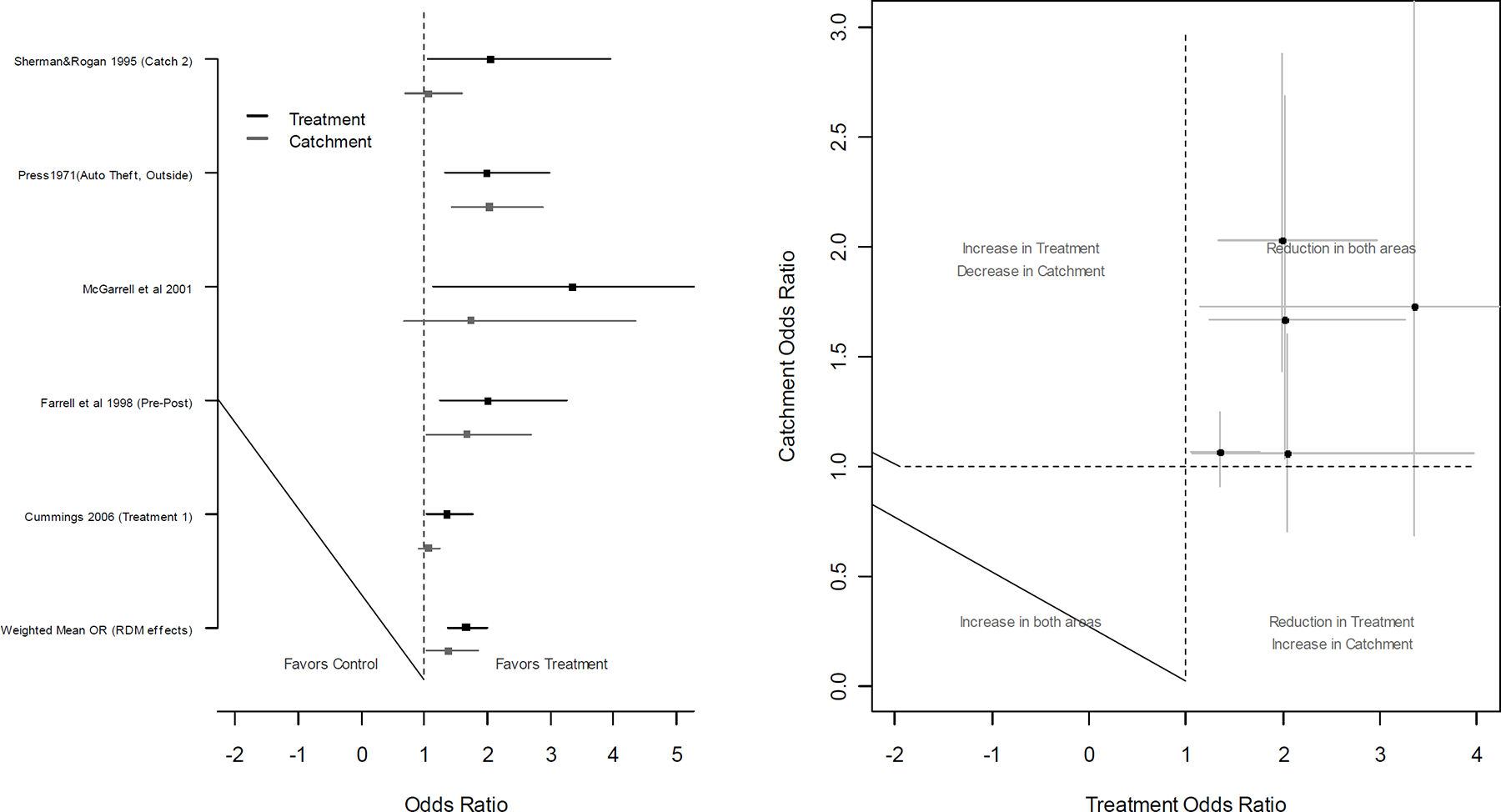
Individual effect size estimates and confidence intervals for the best case scenario across the five quasi-experimental studies for which there was a treatment effect (Left panel), and a scatter plot showing the effect size estimates and confidence intervals for the treatment areas plotted against those for the catchment areas (Right panel)

Figure 7 shows that for worst case scenario a similar pattern emerges but whilst the weighted mean effect size for the treatment areas of 1.50 (CI:1.27-1.78) was statistically significant, for the catchment areas, it was not (M=1.05, CI: 0.89-1.24). Figure 8 shows all eight possible permutations of the data and supports the impression that a reliable treatment effect was observed, and that while crime also reduced in the catchment areas more than elsewhere, this was not apparent for all possible contrasts.

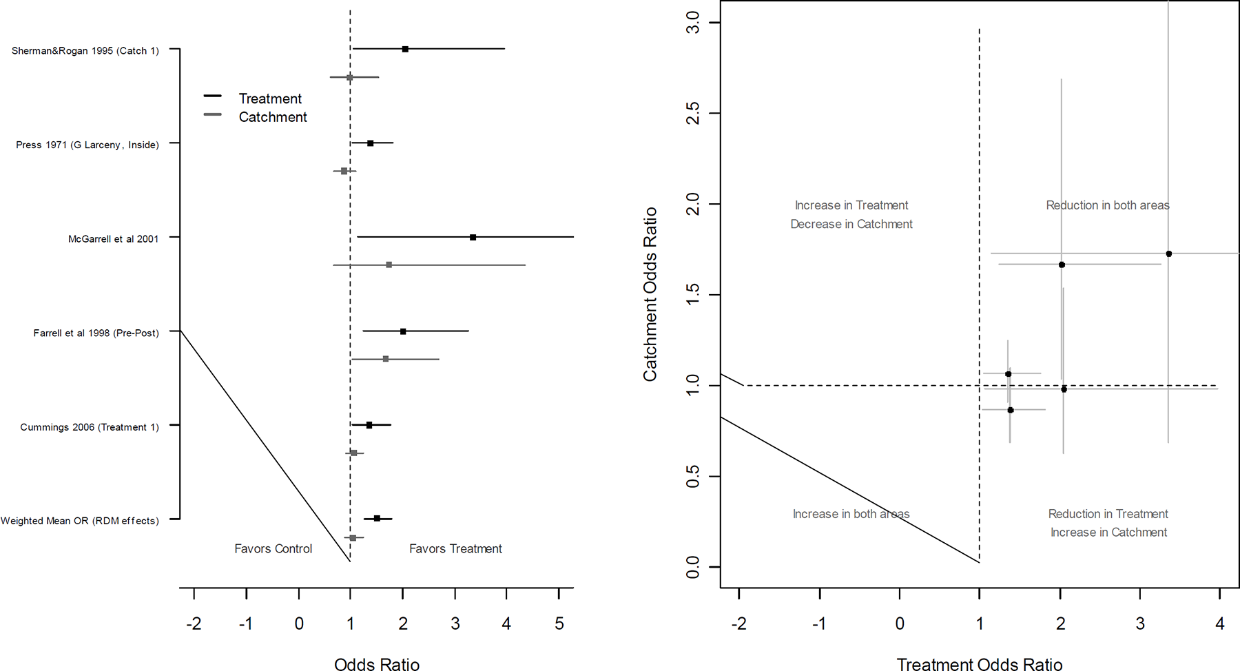
Individual effect size estimates and confidence intervals for the worst case scenario across the five quasi-experimental studies for which there was a treatment effect (Left panel), and a scatter plot showing the effect size estimates and confidence intervals for the treatment areas plotted against those for the catchment areas (Right panel)

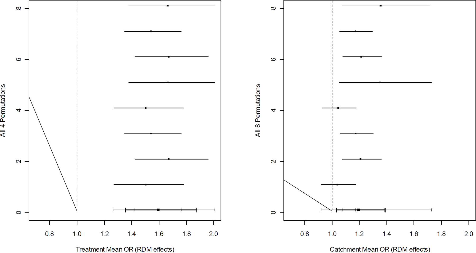
Weighted mean effect size estimates and confidence intervals for the Quasi-Experimental studies that show a treatment effect for the 8 possible permutations, and a summary of that distribution (Left panel: Treatment areas; Right panel: Catchment areas).

For completeness we also present results for all quasi experimental studies, irrespective of whether changes were observed in the treatment areas. In this case, there were a total of 11 studies and 25,920 possible permutations of the data. Figure 9 shows the results for 1000 unique (re)samples of all possible permutations. In this case, there appears to be a positive effect of treatment, although the weighted mean effect is obviously lower than for the subset of schemes considered above. In the case of the catchment areas, while the mean weighted OR is positive, the confidence intervals suggest that the observed trend was unreliable.

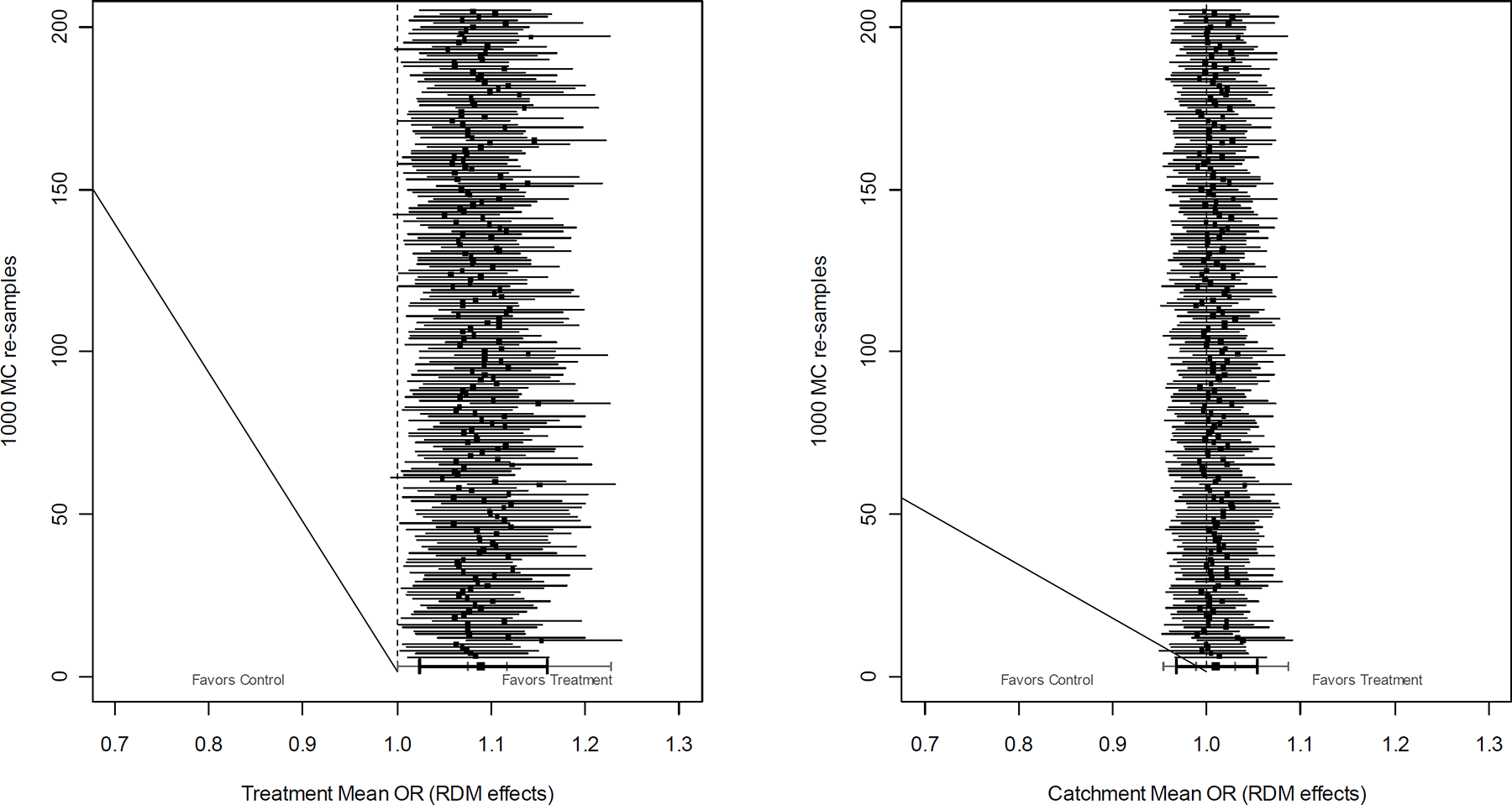
Weighted mean effect size estimates and confidence intervals for Quasi-Experimental studies for 200 of the 1000 Monte Carlo re-samples, and a summary of the distribution for the 1000 samples (Left panel: Treatment areas; Right panel: Catchment areas).

For the quasi-experimental studies then, the conclusions are similar to those for the RCTs. That is, there appears to be a positive effect of treatment for those studies considered and, depending on which studies are examined, the results may be interpreted as suggesting a diffusion of crime control benefit, or little or no change in the catchment areas. In no scenario examined so far, do the results suggest that geographically focused police interventions are generally likely to lead to geographical displacement.

Catchment versus treatment control areas

For four of the five RCT studies and one of the quasi-experimental studies, data were collected for both treatment and catchment control areas. A natural question then is whether the use of the different control areas in the estimates of the effect sizes leads to different conclusions. For two of the studies (Braga, 1999 and Ebensen, 1987) data were available for more than one type of crime and as a result there were 9 pairs of observations in total. Figure 10 shows the pre- and post- monthly counts for the two types of control areas for those studies for which data were available. Visual inspection of the data suggest that with the exception of Braga and Bond (2008) the trends are mostly the same for the two types of control area.

Figures 11 and 12 show the study ORs and confidence intervals for each of the nine possible calculations computed using the catchment control and treatment control areas respectively in the estimation of the ORs for the catchment areas²⁴. In seven of the cases, the individual ORs and confidence intervals were similar irrespective of which control area was used to estimate the effects for the catchment areas. In two of the nine cases (Braga and Bond, 2008 and Braga 1999 – calls for service data), the statistical significance of the ORs changed. For Braga and Bond (2008), the change in the OR for the catchment area was non-significant when the catchment control area was used, but significant when the treatment control area was used. For Braga (1999), when the catchment control area was used the OR was statistically significant, but this was not the case when the treatment control area was used. However, in both cases the conclusion changed from suggesting a diffusion of crime control benefit to a non-significant effect, or vice-versa, rather than switching from suggesting displacement to a diffusion of benefit, or vice-versa. Nevertheless, the finding that the conclusions might vary depending upon the selection of catchment control area suggests that data for catchment control areas should be collected in future studies, where possible.

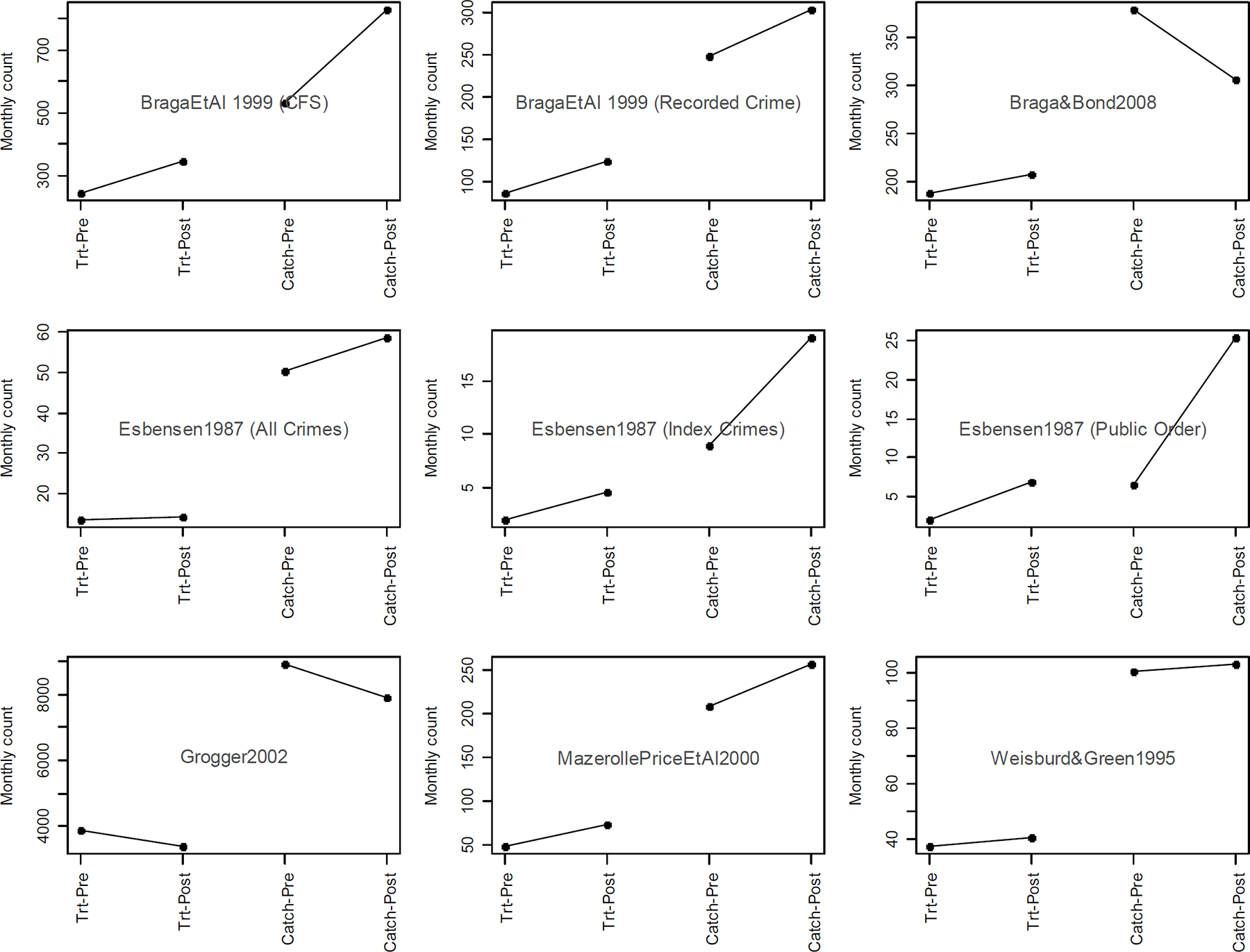
Monthly counts in treatment and catchment control areas for studies which report both

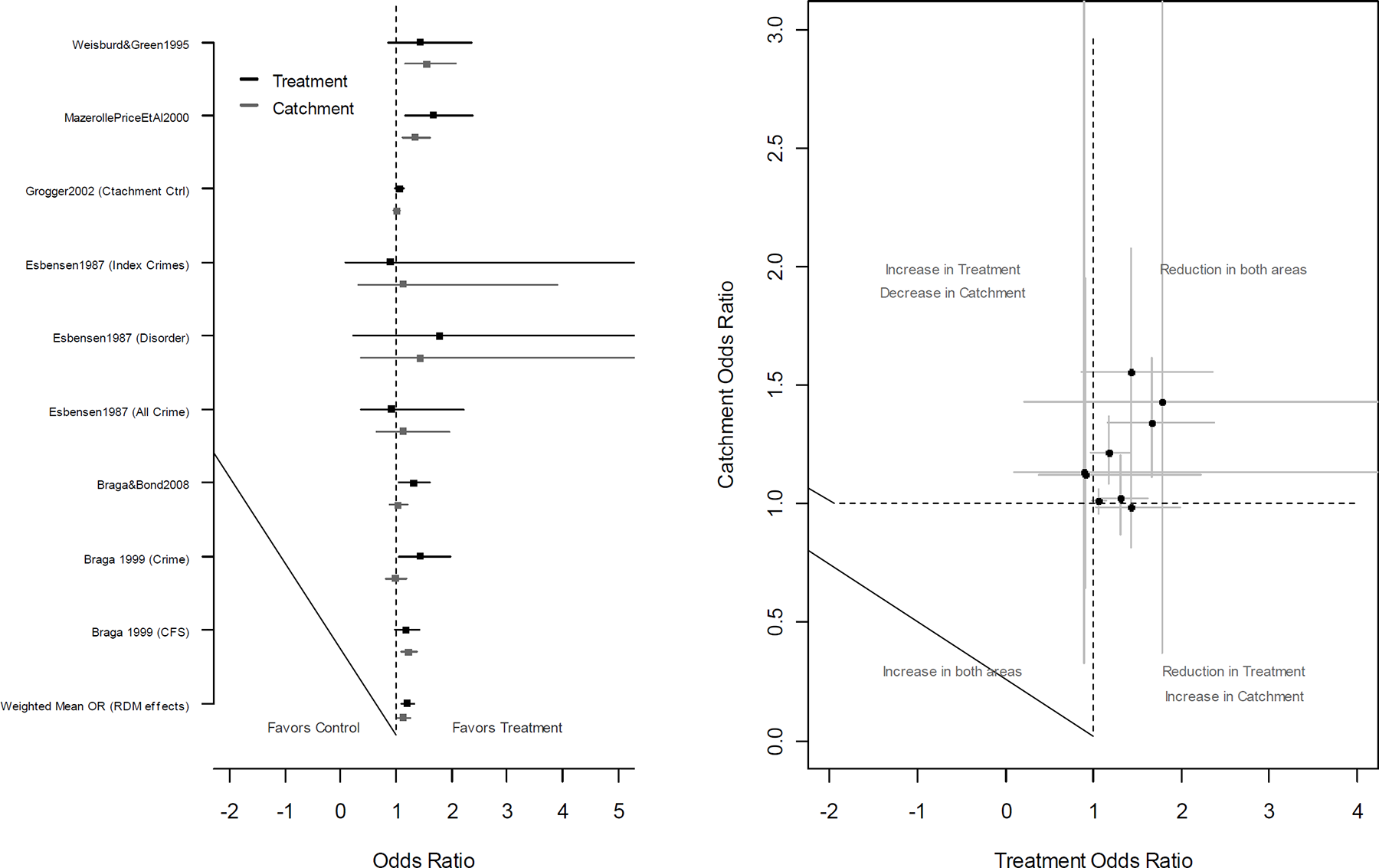
Individual effect size estimates and confidence intervals computed using the catchment control areas for those studies that collected data for both treatment and catchment control areas

Intervention Size

A further way of meaningfully categorizing the studies is in terms of the geographical area they cover. For example, it is possible that interventions that have the largest geographical coverage are least likely to displace crime. That is, in such areas if offenders were deterred by an intervention they might have to travel considerable distances to seek out new opportunities; something that ethnographic research suggests is the exception to the rule (e.g. Rengert and Wasilchick, 1995). Accordingly, we performed separate analyses for those studies that could be categorized as having a large geographical coverage and those that could be categorized as having a small or medium sized geographic range.

Seven of the studies were categorized as large, and across these studies there were 720 possible permutations of the available data. Figure 13 shows that for the best case scenario, the weighted mean effect size of 1.46 (CI: 1.19-1.80) for the treatment areas was statistically significant, but for the catchment areas, while the effect size of 1.19 (CI: 0.99-1.44) was positive it was marginally non-significant. For the worst case scenario, as shown in Figure 14, the weighted mean effect size of 1.21 (CI: 0.99-1.46) for the treatment areas was marginally non-significant, whilst for the catchment areas there was no trend at all (weighted mean OR=0.98, CI:0.83-1.16).

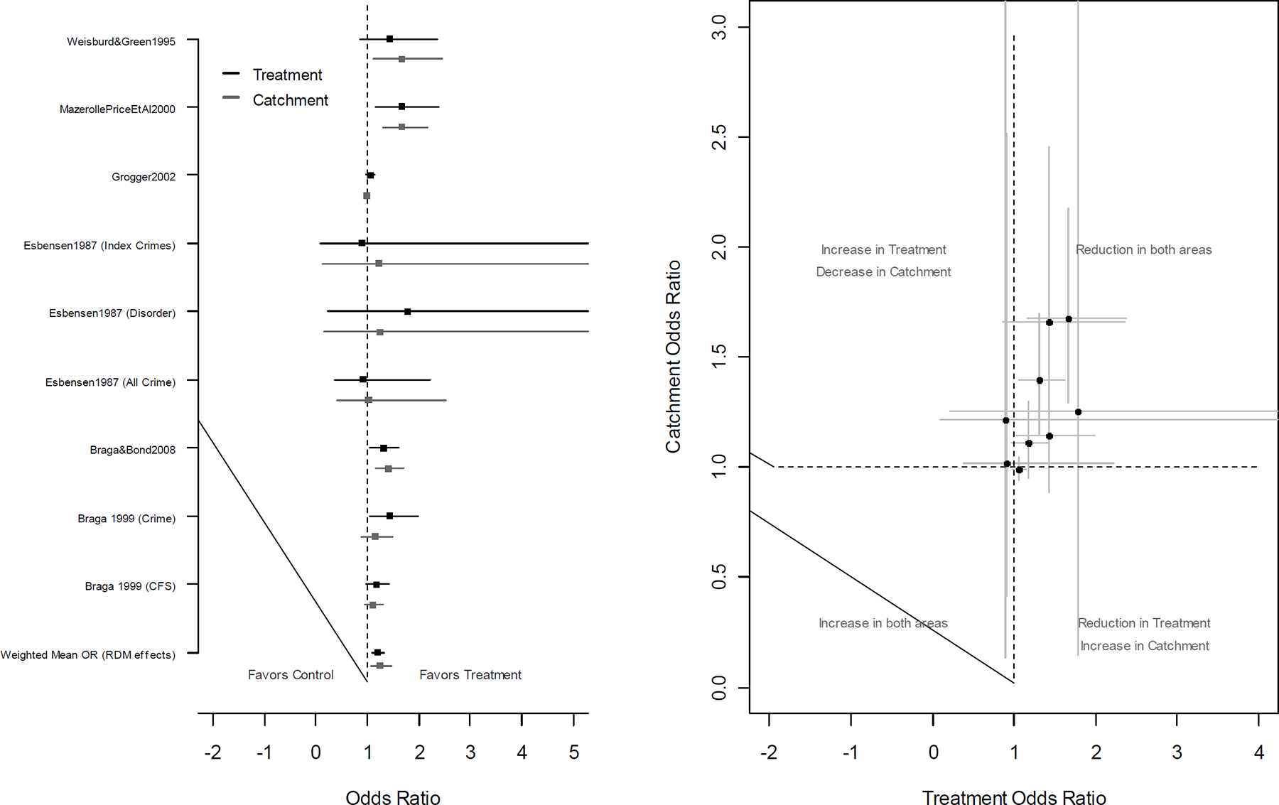
Individual effect size estimates and confidence intervals computed using the treatment control areas for those studies that collected data for both treatment and catchment control areas

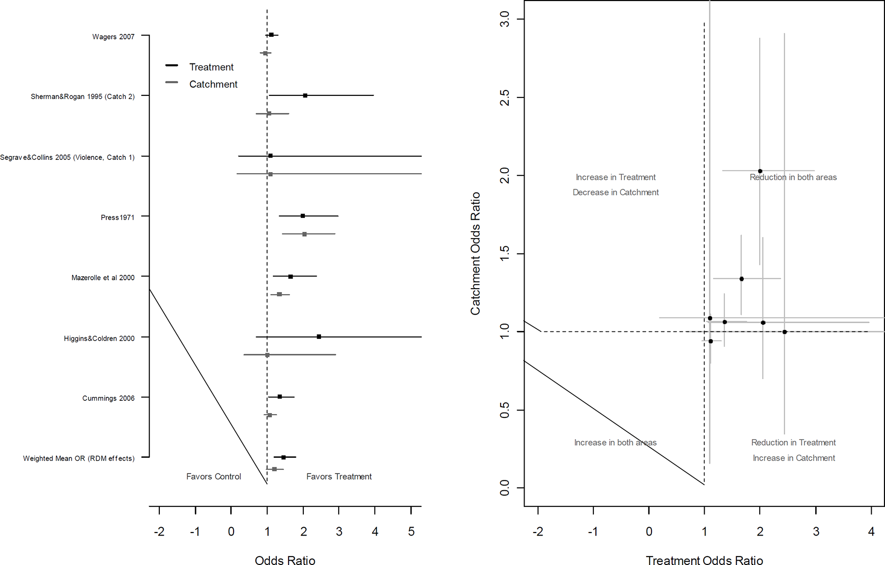
Individual effect size estimates and confidence intervals for the best case scenario for the seven studies that were categorized as large (Left panel), and a scatter plot showing the effect size estimates and confidence intervals for the treatment areas plotted against those for the catchment areas (Right panel)

Figure 15 shows a summary of the results for all 720 permutations. Again, the results suggest a positive effect of treatment, and if anything a trend in favour of a diffusion of crime control benefits albeit non-significant.

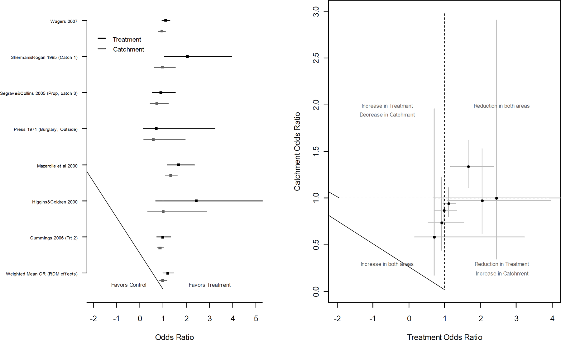
Individual effect size estimates and confidence intervals for the worst case scenario for the seven studies that were categorized as large (Left panel), and a scatter plot showing the effect size estimates and confidence intervals for the treatment areas plotted against those for the catchment areas (Right panel)

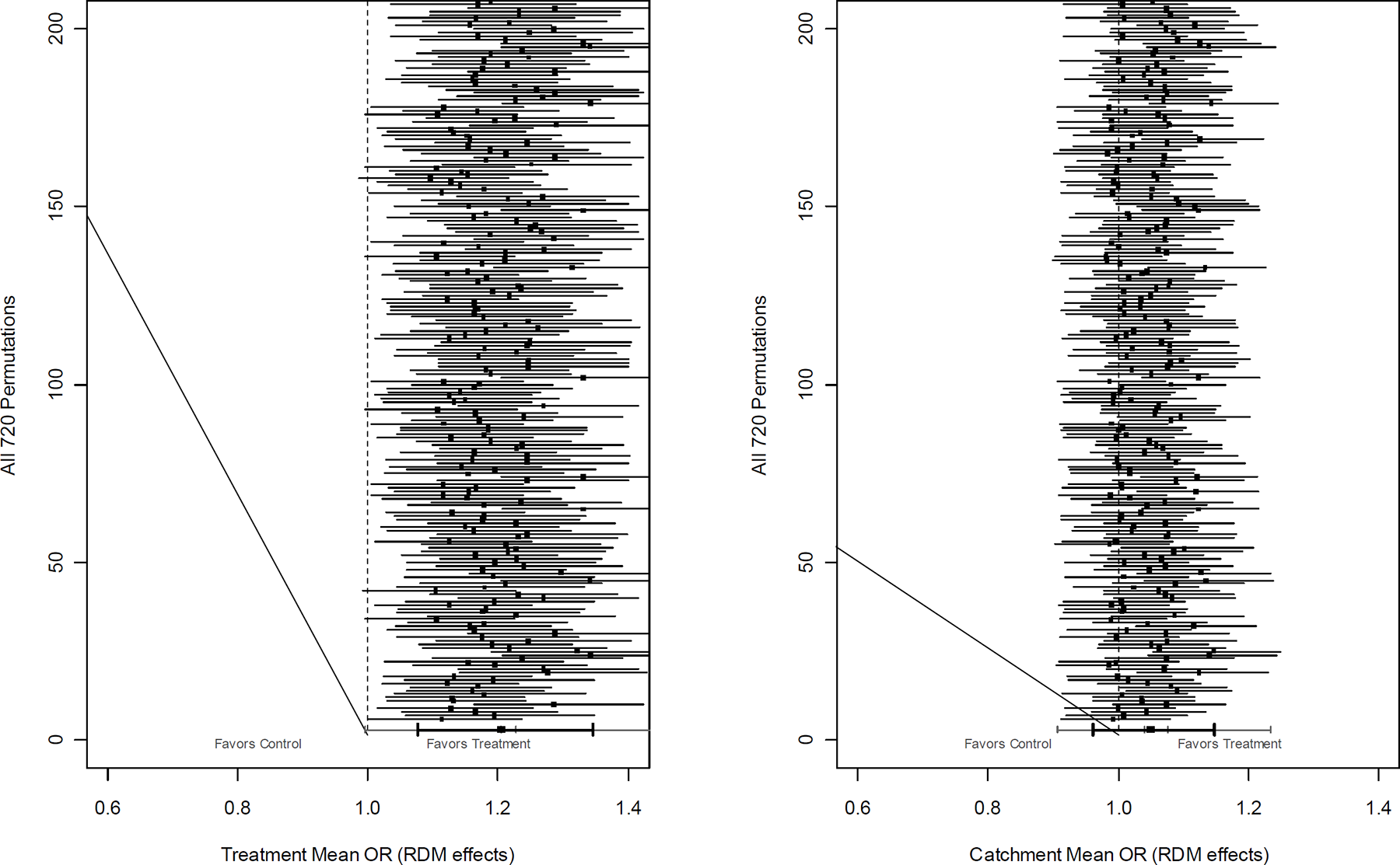
Weighted mean effect size estimates and confidence intervals for studies for which the geographical range of the intervention was categorized as large. Results are for 200 of the 720 possible permutations of the data, and a summary of the distribution for the 720 permutations (Left panel: Treatment areas; Right panel: Catchment areas).

The areas described in six of the studies were classified as medium. Figure 16 shows the results for the best case scenario for this selection of studies. The weighted mean effect size of 1.27 (CI: 1.05-1.54) for the treatment areas was statistically significant, but for the catchment areas the value of 1.07 (CI: 0.94-1.22) was not. For the worst case scenario, shown in Figure 17, the findings were similar with the weighted mean effect size for the treatment areas of 1.14 (CI: 1.01-1.29) being statistically significant, but that for the catchment areas of 1.15 (CI: 0.97-1.37) suggested a non-significant trend. For these studies, there were a total of 16 possible permutations of the data. The results for each of these are shown in Figure 18 and the pattern is in line with a reliable treatment effect accompanied by a non-significant trend in favour of a diffusion of benefit.

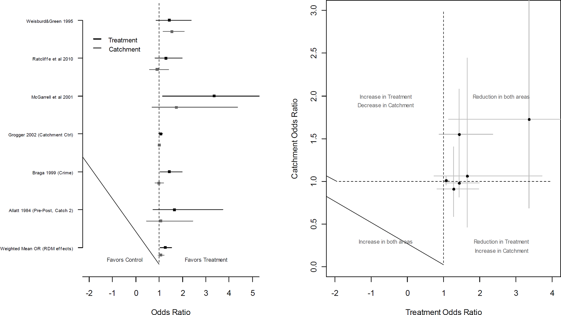
Individual effect size estimates and confidence intervals for the best case scenario for the six studies that were categorized as medium (Left panel), and a scatter plot showing the effect size estimates and confidence intervals for the treatment areas plotted against those for the catchment areas (Right panel)

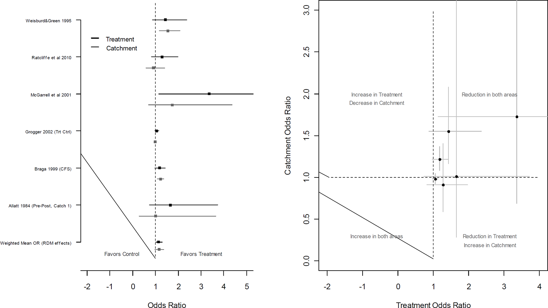
Individual effect size estimates and confidence intervals for the worst case scenario for the six studies that were categorized as medium (Left panel), and a scatter plot showing the effect size estimates and confidence intervals for the treatment areas plotted against those for the catchment areas (Right panel)

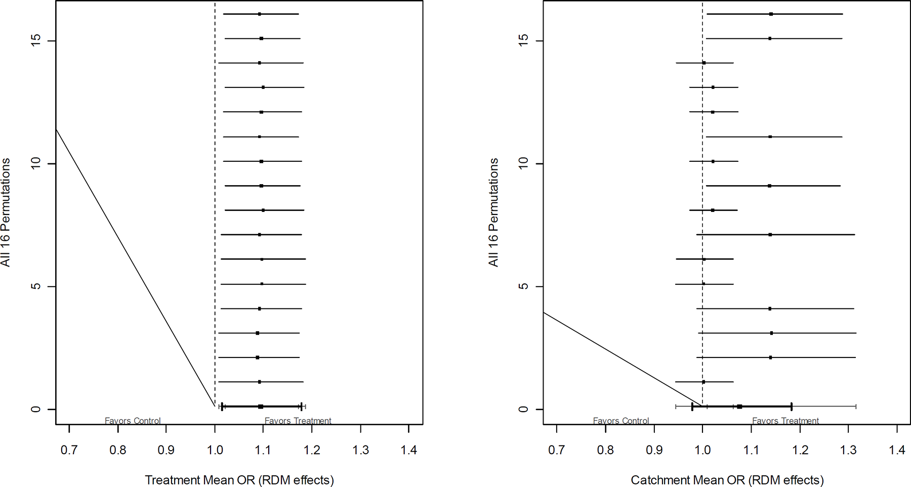
Weighted mean effect size estimates and confidence intervals for studies for which the geographical range of the intervention was categorized as medium. Results are for all 16 possible permutations of the data, and a summary of the distribution (Left panel: Treatment areas; Right panel: Catchment areas).

Only three of the studies were classified as evaluating interventions that took place over a small geographic area. Figure 19 shows that for the best case scenario, the weighted mean effect size of 1.40 (CI: 1.15-1.70) was reliable, whereas for the catchment areas the value of 1.08 (CI: 0.93-1.26) was not. Similar results are apparent for the worst case scenario (see Figure 20) for which the weighted mean effect size for the treatment areas was 1.21 (CI: 1.00-1.47) and for the catchment areas it was 1.04 (CI: 0.89-1.21). Figure 21, which shows the results for all six possible permutations of the data, supports the conclusions already discussed. Thus, similar trends appear to emerge, irrespective of the size of the geographic area covered (at least for the classification criteria used here).

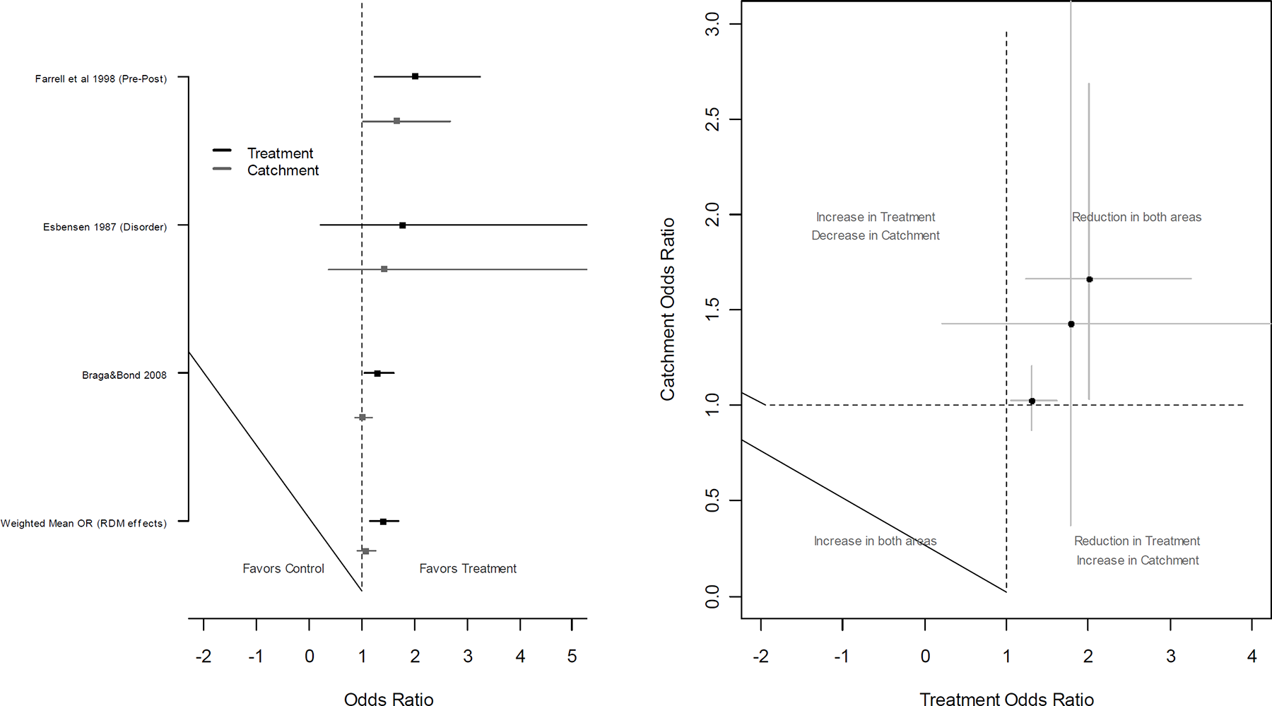
Individual effect size estimates and confidence intervals for the best case scenario for the three studies that were categorized as small (Left panel), and a scatter plot showing the effect size estimates and confidence intervals for the treatment areas plotted against those for the catchment areas (Right panel)

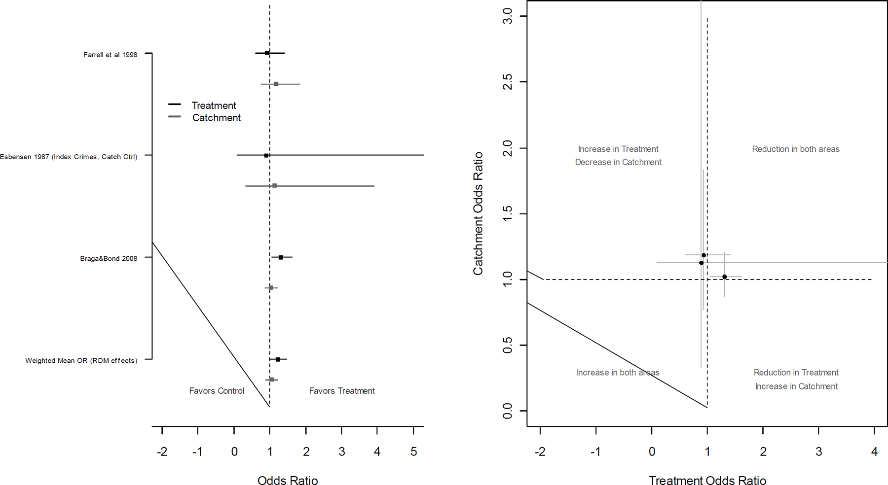
Individual effect size estimates and confidence intervals for the worst case scenario for the three studies that were categorized as small (Left panel), and a scatter plot showing the effect size estimates and confidence intervals for the treatment areas plotted against those for the catchment areas (Right panel)

Intervention type

The interventions employed across the 16 studies were categorized into three broad types: 1) POP and community policing; 2) Increased manpower (hotspots policing, crackdown, foot patrols); and, 3) Other types of focused police-led intervention. Figures 22–24 show the results for those evaluations that were categorized as examining predominantly POP and community policing strategies (N=6). For the best and worst case scenarios, the respective weighted mean effect sizes for the treatment areas of 1.22 (CI: 1.09-1.37) and 1.18 (CI: 1.07-1.30) were statistically significant, while those for the catchment areas - 1.06 (CI: 0.93-1.22) and 1.10 (CI: 0.94-1.27), respectively - were positive but not reliable. Considered alongside those shown in Figure 24, the findings again suggest that overall mean reductions were always observed in both the treatment and catchment areas, although the effects observed in the catchment areas may be due to sampling error rather than a reliable effect of intervention.

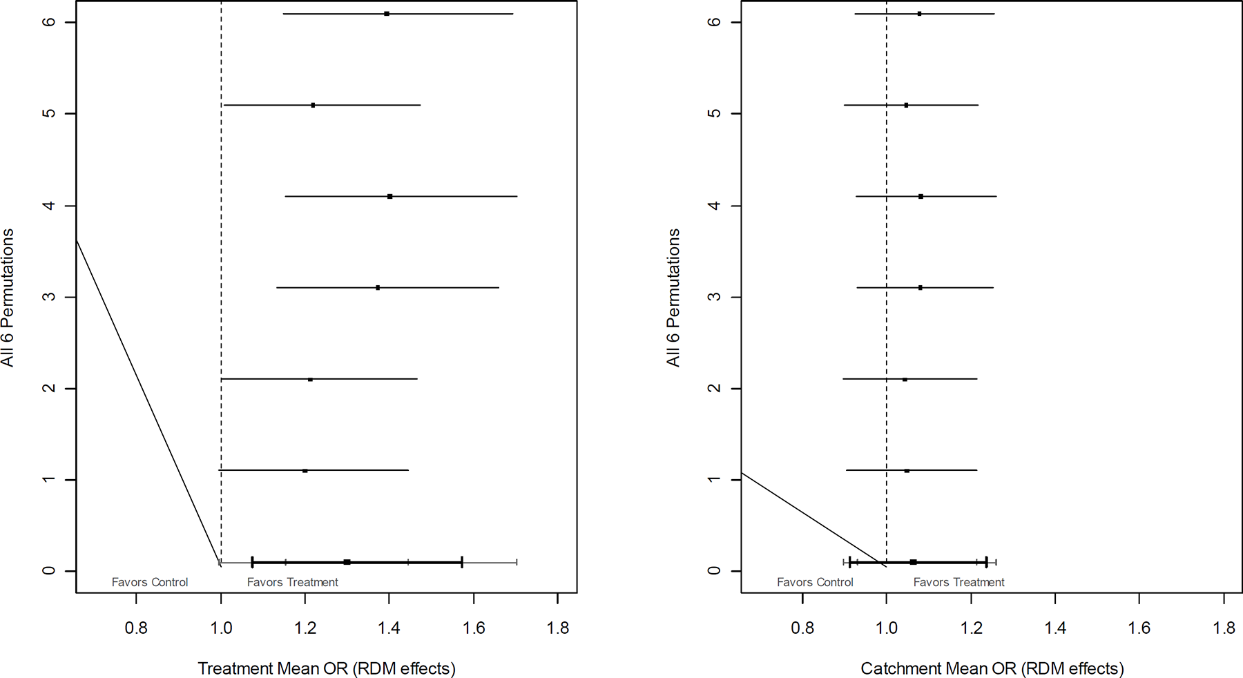
Weighted mean effect size estimates and confidence intervals for studies for which the geographical range of the intervention was categorized as small. Results are for all six possible permutations of the data, and a summary of the distribution for all permutations (Left panel: Treatment areas; Right panel: Catchment areas).

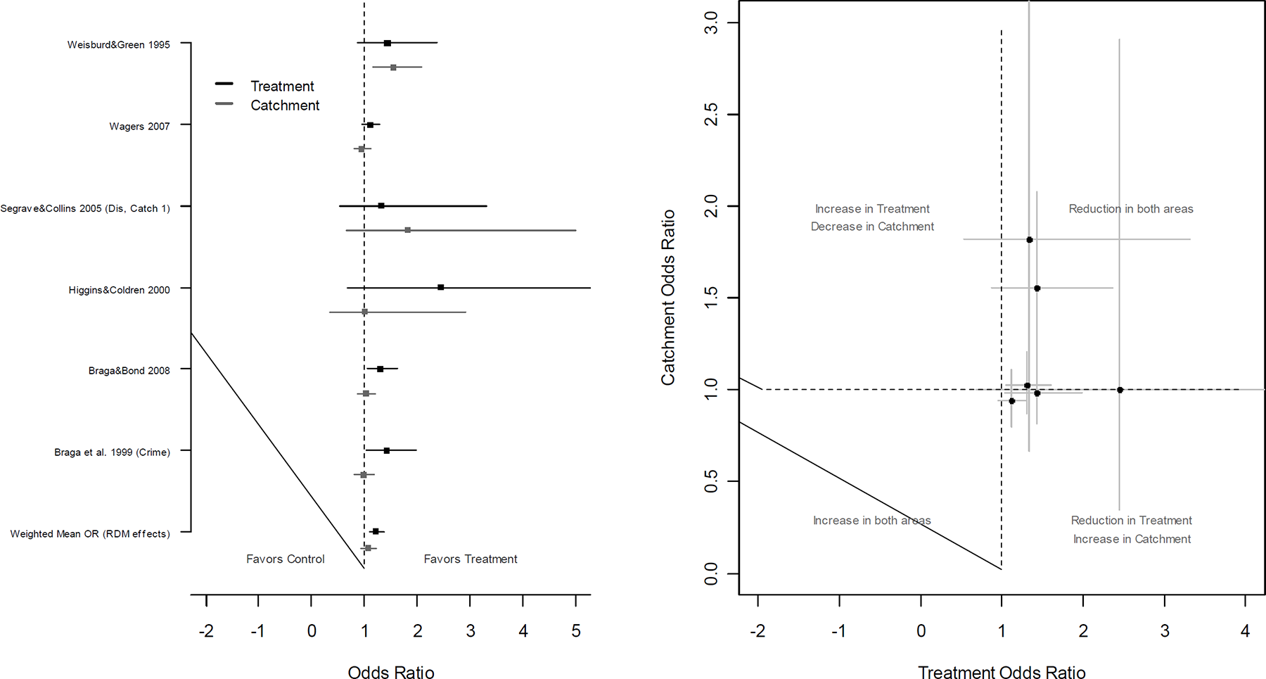
Individual effect size estimates and confidence intervals for the best case scenario for evaluations of POP or community policing interventions (Left panel), and a scatter plot showing the effect size estimates and confidence intervals for the treatment areas plotted against those for the catchment areas (Right panel)

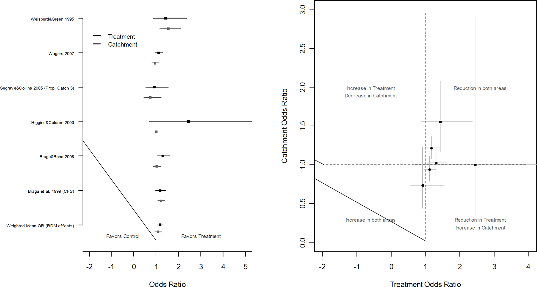
Individual effect size estimates and confidence intervals for the worst case scenario for evaluations of POP or community policing interventions (Left panel), and a scatter plot showing the effect size estimates and confidence intervals for the treatment areas plotted against those for the catchment areas (Right panel)

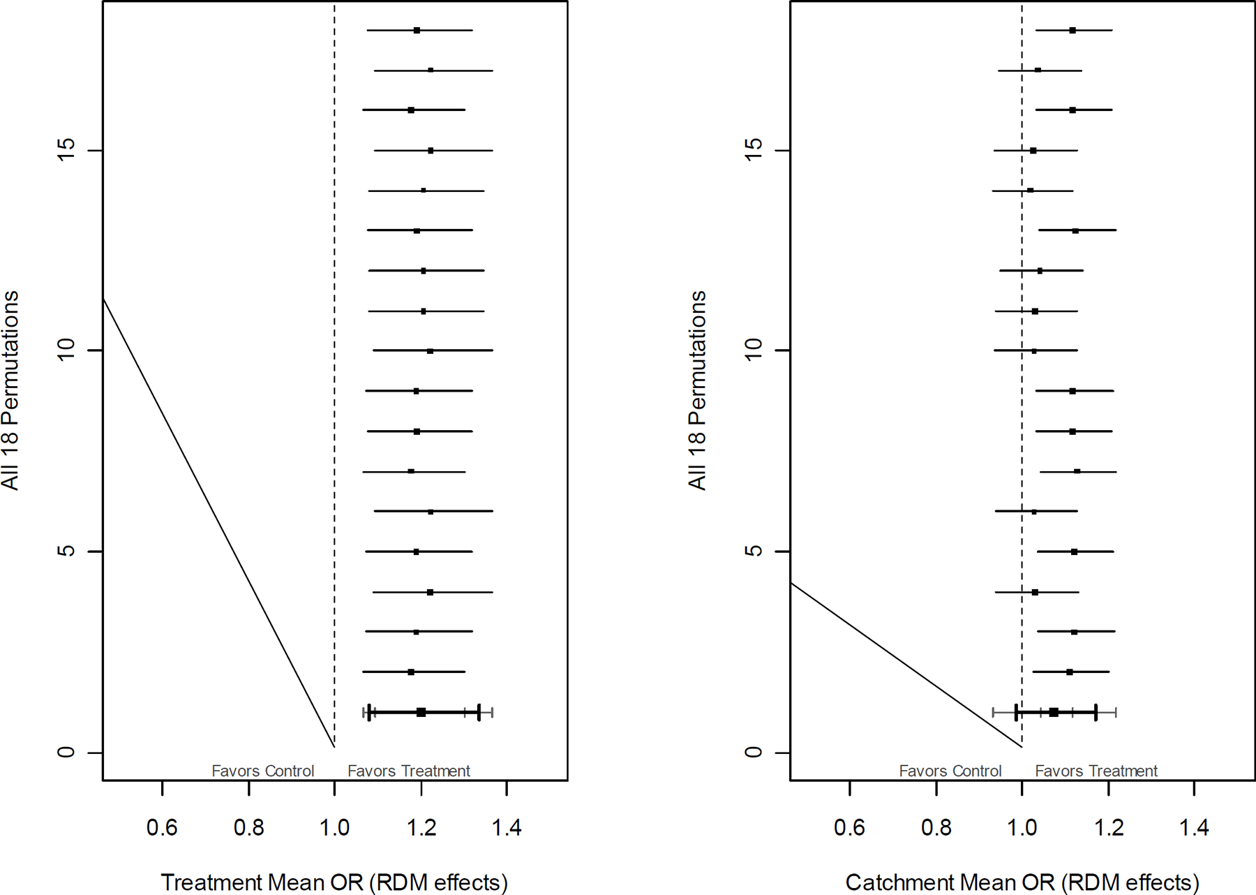
Weighted mean effect size estimates and confidence intervals for evaluations of POP or community policing interventions. Results are for all 18 possible permutations of the data, and a summary of the distribution for all permutations (Left panel: Treatment areas; Right panel: Catchment areas).

Figures 25–27 show the same analyses for those studies in which the predominant strategy was to increase manpower in a geographically focused area (N=8). Here, there appears to be a positive effect in the treatment areas for the best (weighted mean OR=1.54, CI: 1.18-2.01) but not for the worst case scenario (weighted mean OR=1.13, CI: 0.98-1.29). Apropos changes observed in the catchment areas, no reliable effect was observed for the best case scenario (weighted mean OR=1.25, CI: 0.97-1.60) but a trend in favour of displacement was noted for the worst case scenario (weighted mean OR=0.93, CI: 0.84-1.03). However, inspection of Figure 27, which shows the results for all 480 possible permutations of the data, suggests that the trend observed was atypical and that the most likely outcome was for there to be no change in the catchment areas.

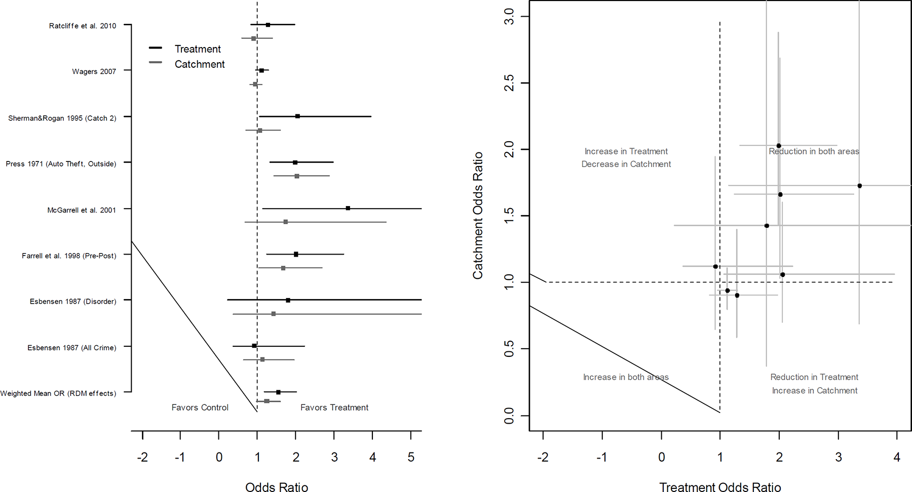
Individual effect size estimates and confidence intervals for the best case scenario for evaluations of geographically focused interventions that employ increased manpower (Left panel), and a scatter plot showing the effect size estimates and confidence intervals for the treatment areas plotted against those for the catchment areas (Right panel)

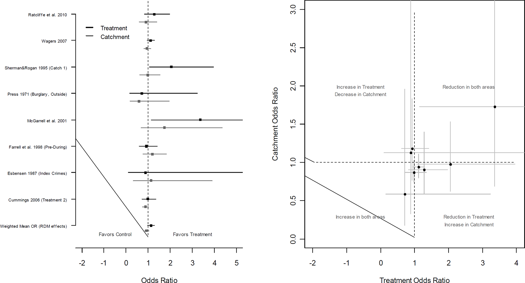
Individual effect size estimates and confidence intervals for the worst case scenario for evaluations of geographically focused interventions that employ increased manpower (Left panel), and a scatter plot showing the effect size estimates and confidence intervals for the treatment areas plotted against those for the catchment areas (Right panel)

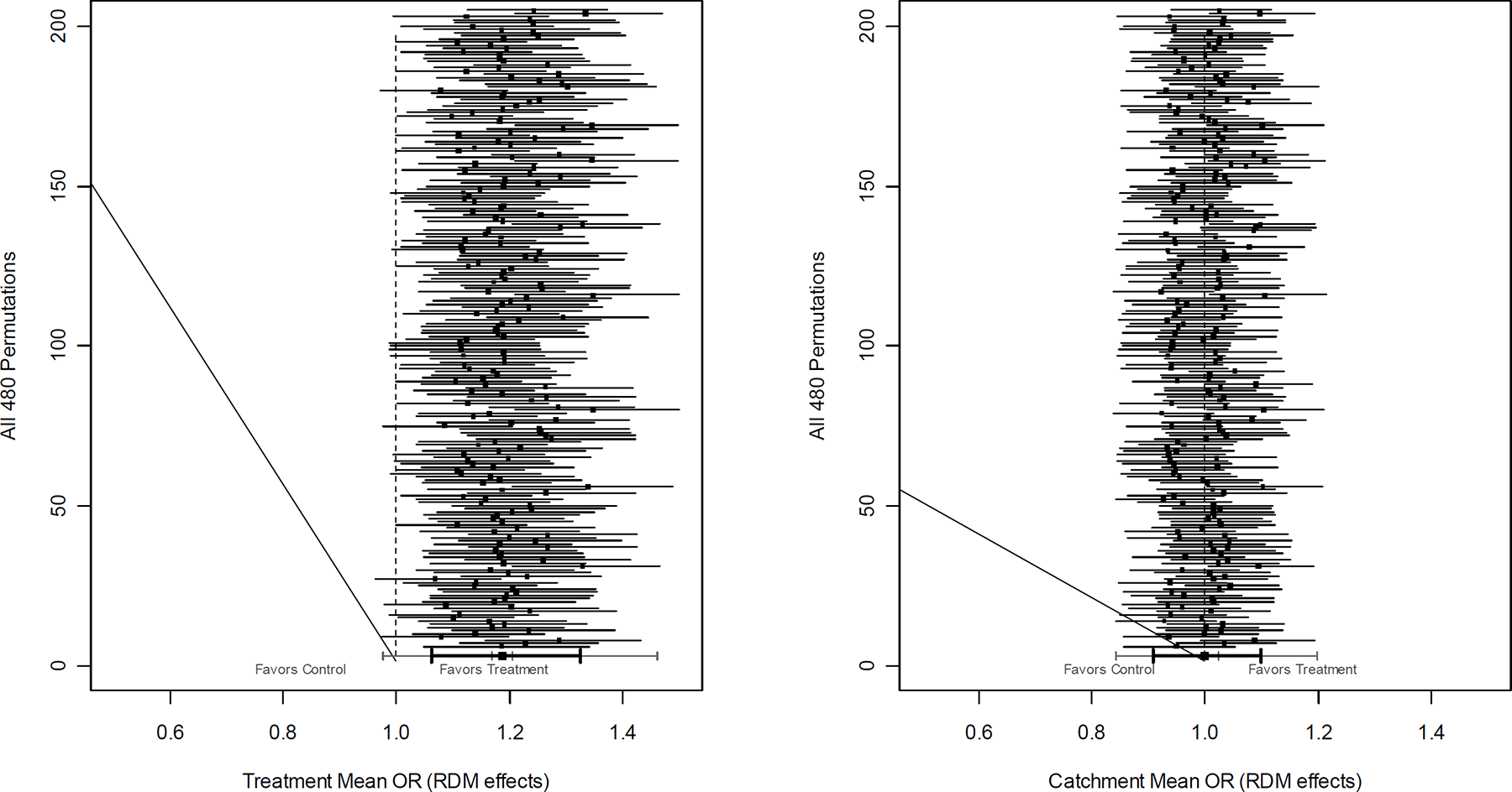
Weighted mean effect size estimates and confidence intervals for evaluations of geographically focused interventions that employ increased manpower. Results are for all 480 possible permutations of the data, and a summary of the distribution for all permutations (Left panel: Treatment areas; Right panel: Catchment areas).

Finally, Figures 28–30 shows the results for other types of police led intervention (N=4). The results were similar for this type of strategy. However, for both the best (weighted mean OR=1.34, CI: 0.98-1.83)²⁵ and worst case (weighted mean OR=1.26, CI: 0.94-1.67) scenarios the treatment effect was positive but marginally non-significant. With respect to the catchment areas, for both the best (weighted mean OR=1.12, CI: 0.94-1.34) and worst case scenarios (weighted mean OR=1.11, CI: 0.90-1.38) there was also a non-significant trend which suggested that crime reduced in the catchments areas, although the effect size was smaller as well as being non-significant. Analysis of all eight possible permutations of the data provides a picture consistent with the above conclusions.

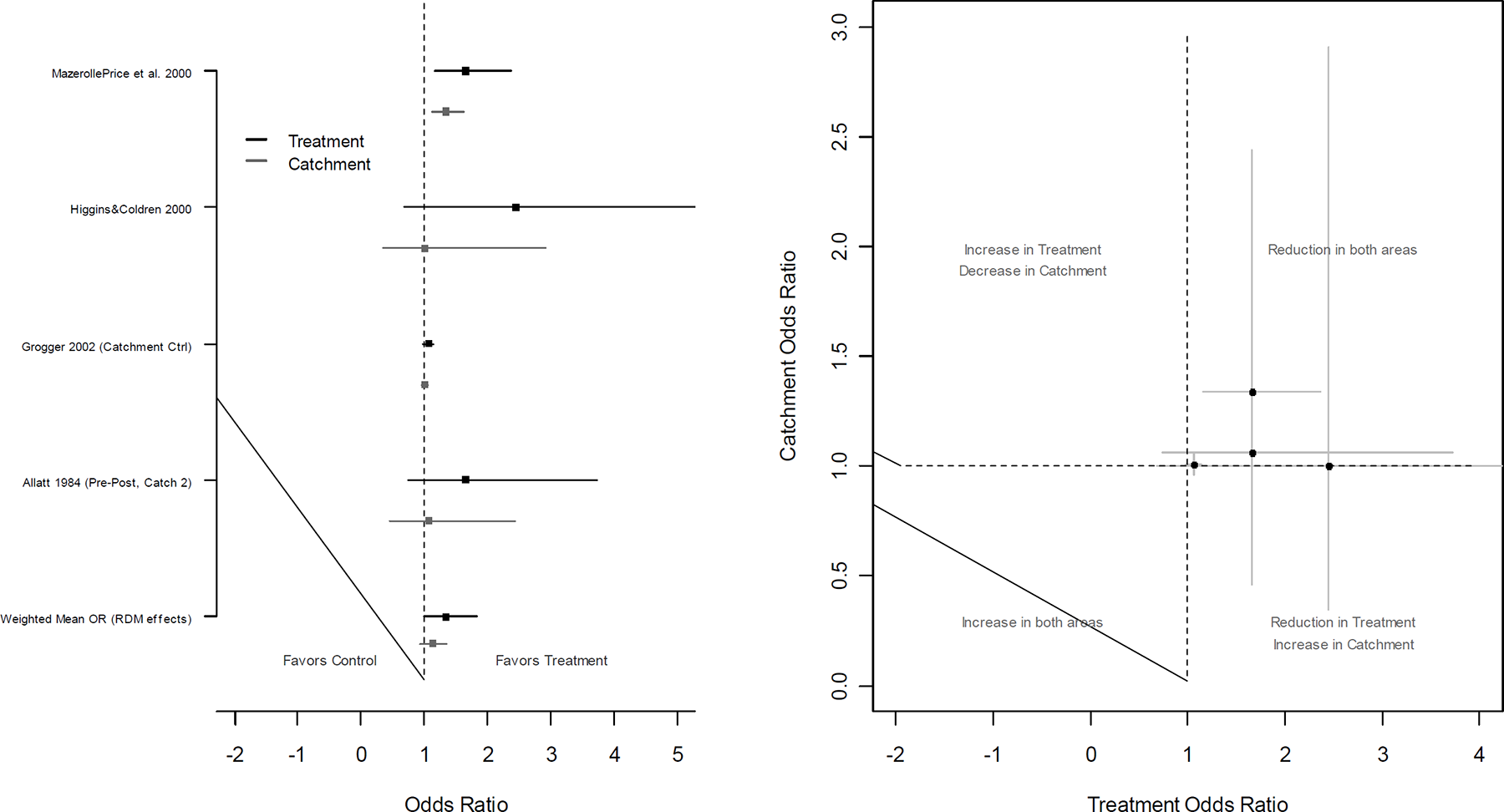
Individual effect size estimates and confidence intervals for the best case scenario for evaluations of police-led initiatives that employ “other” types of interventions (Left panel), and a scatter plot showing the effect size estimates and confidence intervals for the treatment areas plotted against those for the catchment areas (Right panel)

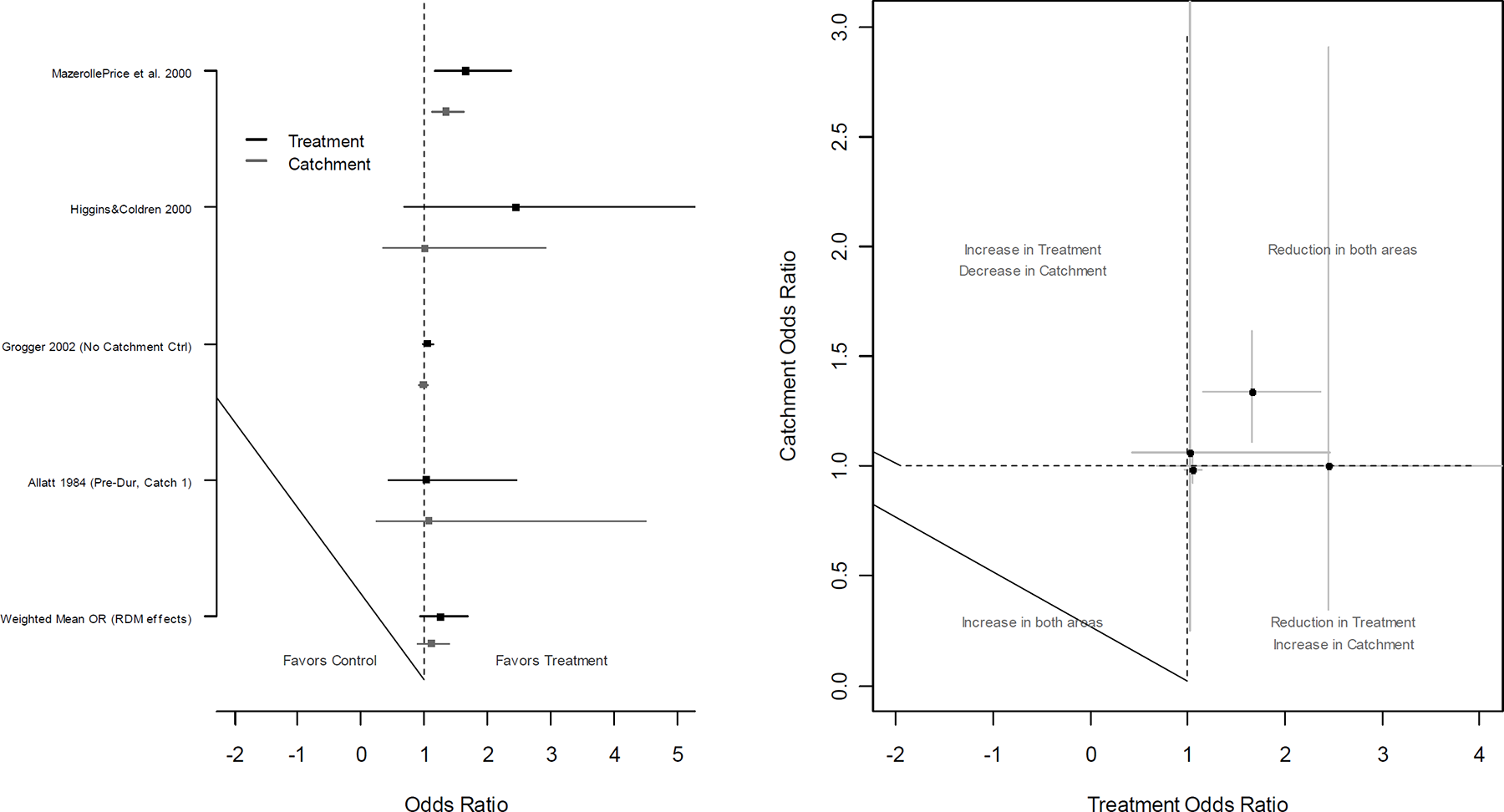
Individual effect size estimates and confidence intervals for the worst case scenario for evaluations of police-led initiatives that employ “other” types of interventions (Left panel), and a scatter plot showing the effect size estimates and confidence intervals for the treatment areas plotted against those for the catchment areas (Right panel)

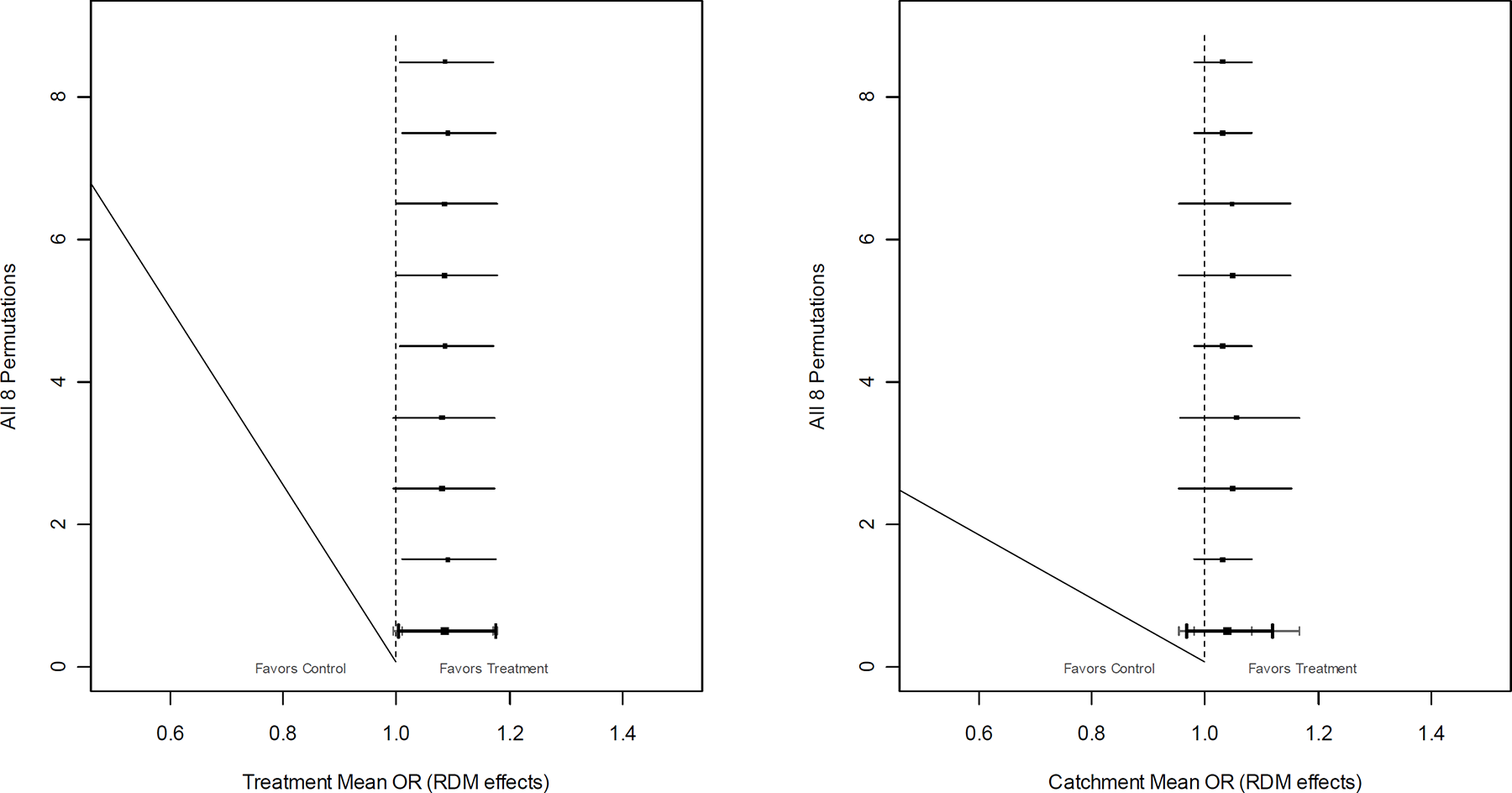
Weighted mean effect size estimates and confidence intervals for evaluations of police-led initiatives that employ “other” types of interventions. Results are for all 8 possible permutations of the data, and a summary of the distribution for all permutations (Left panel: Treatment areas; Right panel: Catchment areas).

Publication bias

Only three of the studies were unpublished at the time of writing. Of these, one is currently submitted to a journal and so it would be improper to assign it to one category or the other at this stage. Of the two remaining studies (Wagers, 2007; Higgins & Coldren, 2000), both suggested a reduction in the treatment areas but this was non-significant. For one the change in the catchment area was neither positive nor negative (Higgins & Coldren, 2000), and for the other (Wagers, 2007) there was an increase in crime in the catchment area but this trend was not statistically significant.

A variety of procedures are available to examine the possible effects of publication bias and here, like Weisburd et al 2008, we use the trim and fill algorithm proposed by Duval and Tweedie (2000). Figure 31 show the results of this analysis, which was only possible to conduct on the 16 studies that were used in the meta-analysis, for which numeric effect sizes had been calculated. The key principle is that in the absence of bias, the funnel plots shown, which in this case chart the standard error on the x-axis against the effect size (log odds ratio) on the y-axis, would be symmetric around the mean effect size. If there are more studies above than below, our concern is that we have missing studies from below, which seem likely to be the unpublished ones. In these figures, which were produced in STATA, the circles represent the original points as circles, and those imputed from the trim and fill procedure as circles within squares. The points are imputed using an iterative procedure which continues until the funnel plot can become symmetric. This yields an adjusted estimate of effect size.

Figure 31 summarises the trim and fill results for four scenarios. Figure 31(a) shows that for the best case scenario for treatment areas, 8 studies are suggested as missing. The original point estimate in log units was 0.337, which corresponds to a risk ratio of 1.40. The adjusted point estimate is 0.193, which is an odds ratio of 1.21. Figure 31(b) shows that for the worst case scenario for treatment areas, one study is suggested as missing. The original point estimate in log units was 0.156, which corresponds to a risk ratio of 1.17. The adjusted point estimate is 0.151, which is an odds ratio of 1.16. Figure 31(c) shows that for the best case scenario for catchment areas, 3 studies are suggested as missing. The original point estimate in log units was 0.136, which corresponds to a risk ratio of 1.15. The adjusted point estimate is 0.093, which is an odds ratio of 1.10. Figure 31(d) shows that for the worst case scenario for catchment areas, no studies are suggested as missing. The original point estimate in log units was 0.068, which corresponds to a risk ratio of 1.07. The adjusted point estimate remains the same in this case.

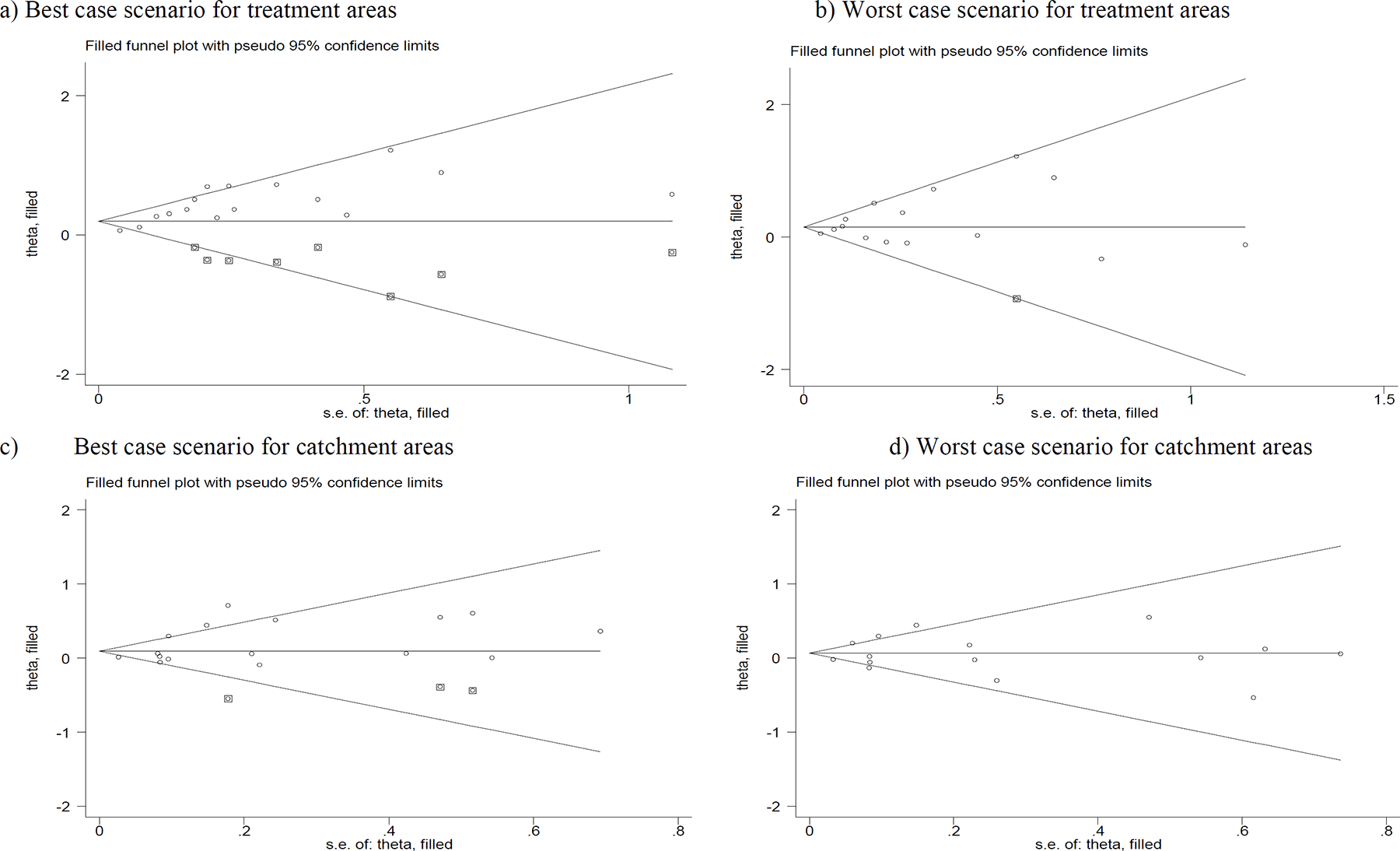
Funnel plots with trim and fill imputations for:

These results demonstrate that in general, accounting for publication bias does not seem to effect the initial conclusions of the meta-analysis; the adjusted effect size estimates are fairly similar to the original ones. The slight exception to this is for the best case scenario for the treatment areas where there is a drop in the odds ratio. Here, even the adjusted effect size continues to demonstrate a significant effect of treatment. It appears therefore, that publication bias is not a major concern for this analysis.

As pointed out by Weisburd et al (2008) this method could be misleading in the context of this particular study. This is because it is entirely possible that smaller studies (those with a larger standard error) might well be expected to produce average, or even larger than average effect sizes. It could be that the smaller the areas that are policed, the less stretched and more focused the operational resources. Furthermore, it is unreasonable to assume that the studies are a homogenous population. As we have seen they vary in their methodological approach, their context and their objectives, and so it is unrealistic to put any asymmetry down to sampling error alone (Rothstein 2008).

Summary of the meta-analysis

In short, the weight of the evidence suggests that irrespective of how the data are grouped, geographically focused interventions do not generally displace crime to nearby areas. Instead, there is a trend which suggests that a crime decreases in such locations.

4.5 Weighted Displacement Quotient and Total Net Effect Analysis

4.5.1 Descriptive Statistics

The formulae used to calculate the descriptive statistics were presented in the methods section. More details regarding the use and interpretation of the GE, NE, WDQ, TNE and Success and Catchment Displacement measures are provided in Appendix F. For the reasons discussed above, these metrics were only computed for those quasi-experimental studies for which there was evidence of a reduction in the treatment areas. The TNE calculations were developed for the analysis of count data and so are reported here. For completeness, estimates for all observations (for which there was a reduction in the treatment areas) included in the meta-analysis are shown in Appendix G. Due to the multiple observations available for some of the studies, this gives a total of 36 different calculations for each of the measures expressed above.

Figure 32 provides a summary of the results of the TNE calculations. The Figure shows that in general there was more suggestion of a positive net effect than a negative one. Furthermore, it seems that where negative effects are observed they are of a considerably smaller magnitude than those where a positive effect is suggested. These results are therefore consistent with those discussed in previous sections; on average it appears that interventions appear successful at reducing crime and the benefit from these successes is often diffused.

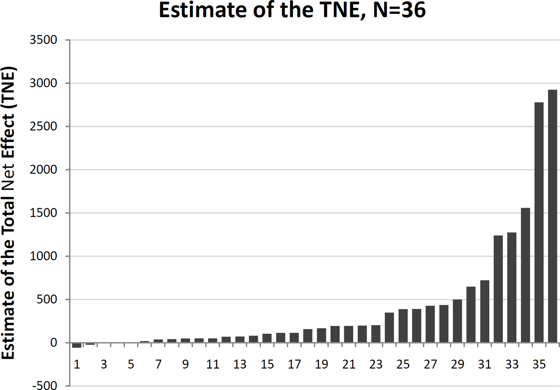
Point estimates of the Total Net Effect (TNE) for 36 observations (from 16 studies)

4.5.2 Weighted Displacement Quotient analysis

Figure 33 shows the results of the modified WDQ analysis for the best- and worst-case scenarios. The weighted mean effects are calculated in the same way as in previous sections. In the worst case scenario, there is only one study for which the 95 percent confidence intervals are to the left of the null effect line of zero. For the same scenario, there are three cases where they are to the right of it. For the remainder, the confidence intervals overlap the null effect line of zero. Overall, for this scenario the WDQ is positive, although the confidence intervals overlap the line of null effect. For the best-case scenario the weighted mean effect size is above 0 and the confidence intervals do not overlap the null effect line. In summary, the weighted mean WDQ for both the best- and worst-case scenarios suggest that a diffusion of benefit is the most likely outcome of geographically focused initiatives.

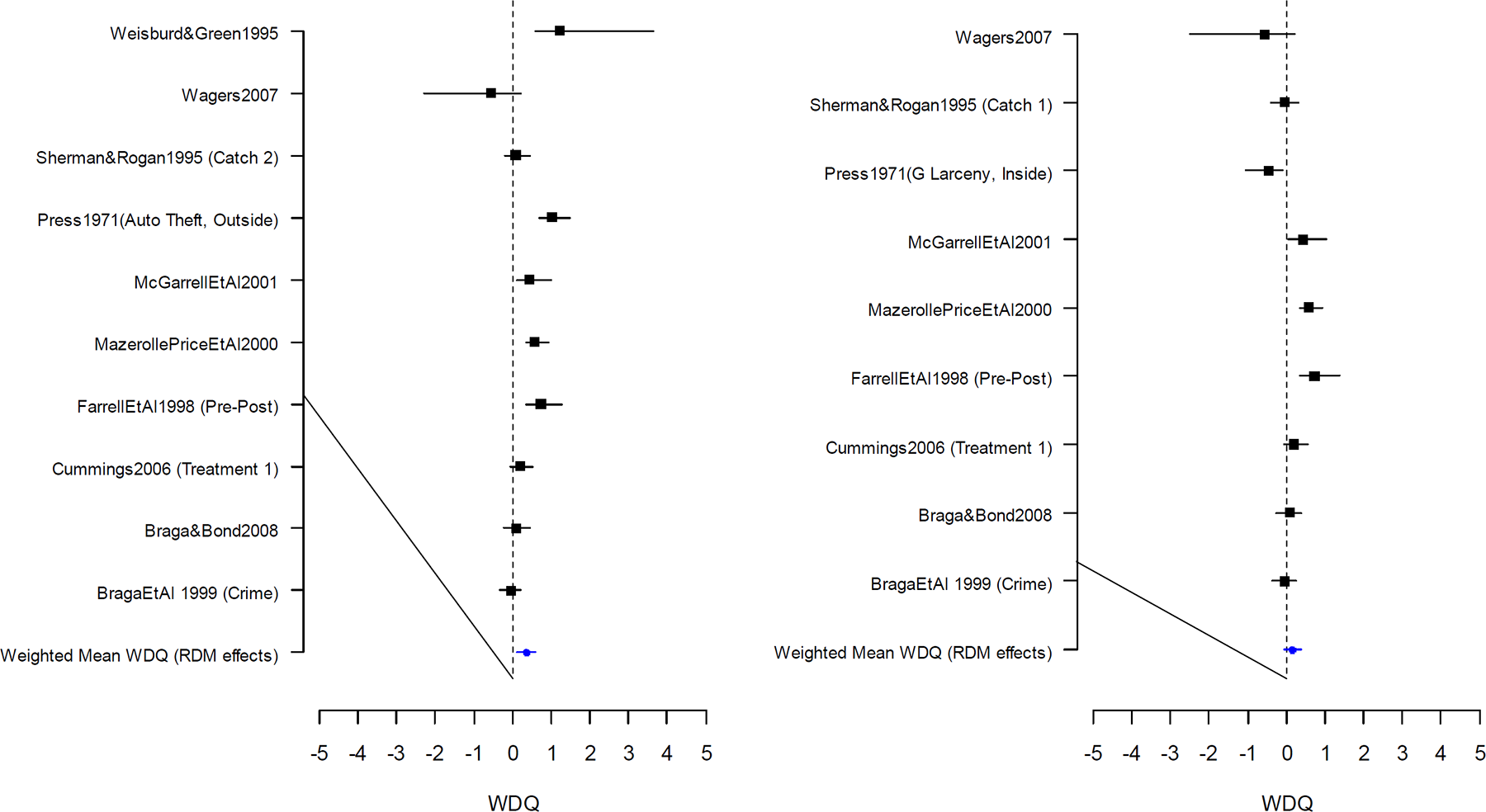
Best and worst case scenarios for the weighted displacement quotient analysis (Note: values above one show a possible diffusion of benefit, values less than one potential displacement)

4.6 Pre-post studies

For 36 of the 44 studies which met the study criteria, count data were available, or it was possible to estimate counts from the information reported in the research paper. These included the 16 studies that were entered into the meta-analysis. For these data, counts before and after intervention for the treatment area(s) and catchment area(s) were used to generate proportional change figures. For this analysis, we ensured that the figures accounted for any differences in the duration of the ‘before’ and ‘after’ periods. The results are summarized in Figure 34. In each case, the proportional change in the treatment and catchment area are shown next to each other. Where the observed change is to the right (left) of the zero line this indicates that crime increased (decreased) in the area. The Figure is rank-ordered by the proportional changes observed in the treatment areas (from the largest increase to largest decrease). For the majority of studies there was a decrease in crime in both the treatment and catchment areas. This is in line with the previous suggestion that on the whole the interventions reduced crime in the treatment areas and did not displace it to nearby areas.

Figure 34 also appears to indicate some correspondence between the change in the treatment areas and the change in the catchment areas. Reductions in the treatment area are often mirrored by reduction in the catchment areas as well. There does not appear to be a systematic relationship between the size of the change in the two area types.

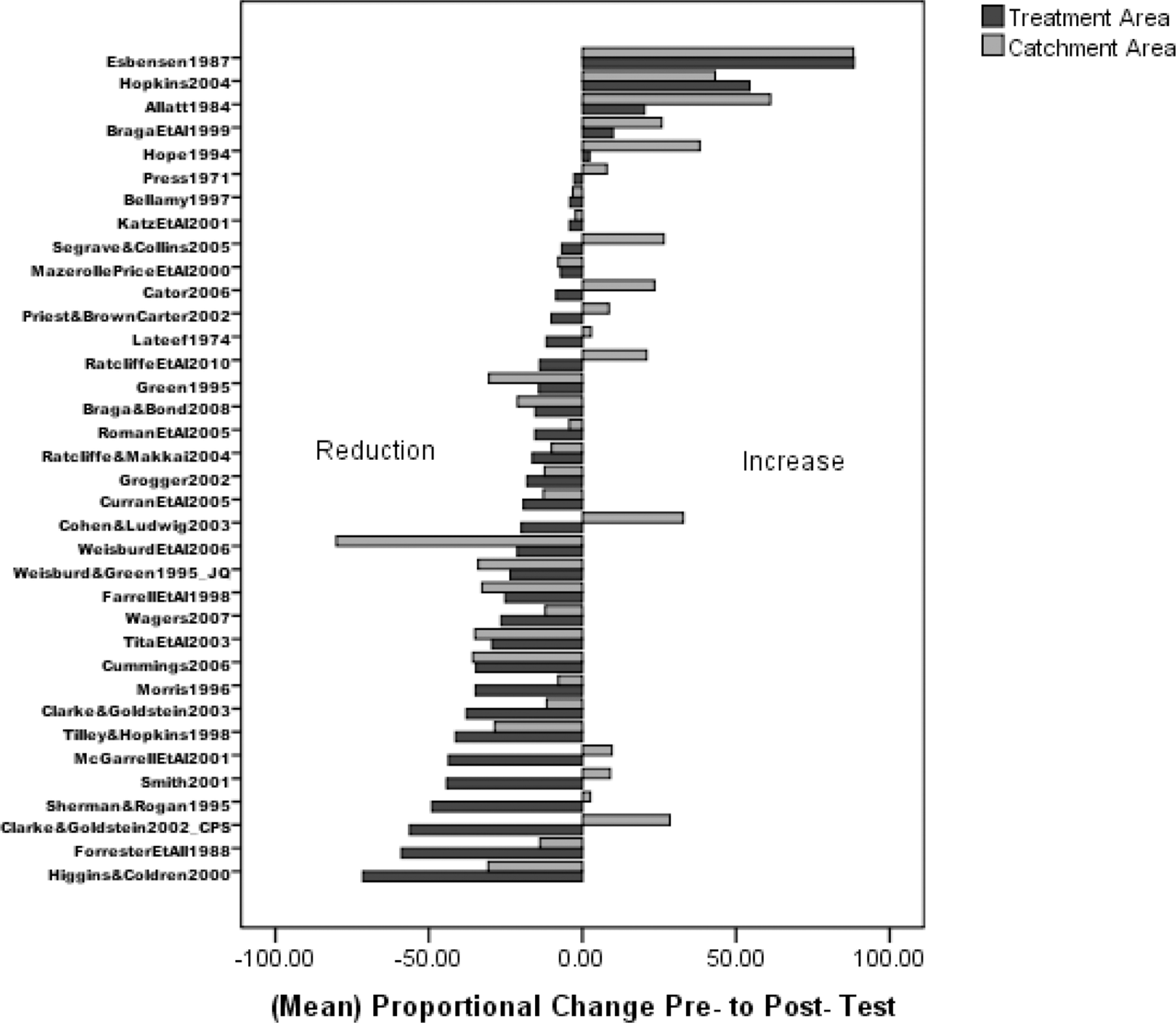
Proportional Change Pre to Post test for treatment and catchment areas (N=36)

Figure 35 shows the proportional change for larger and smaller initiatives separately. There do not appear to be obvious differences in observed trends for studies where the intervention covered a larger geographic area and those where coverage more limited. If anything, it appears that the studies which evaluated interventions with a larger geographic coverage experienced greater reductions in the treatment and catchment areas than those with smaller coverage. However, it is important to note that for the analyses presented in this section, the changes observed were not contrasted with changes in suitable control areas.

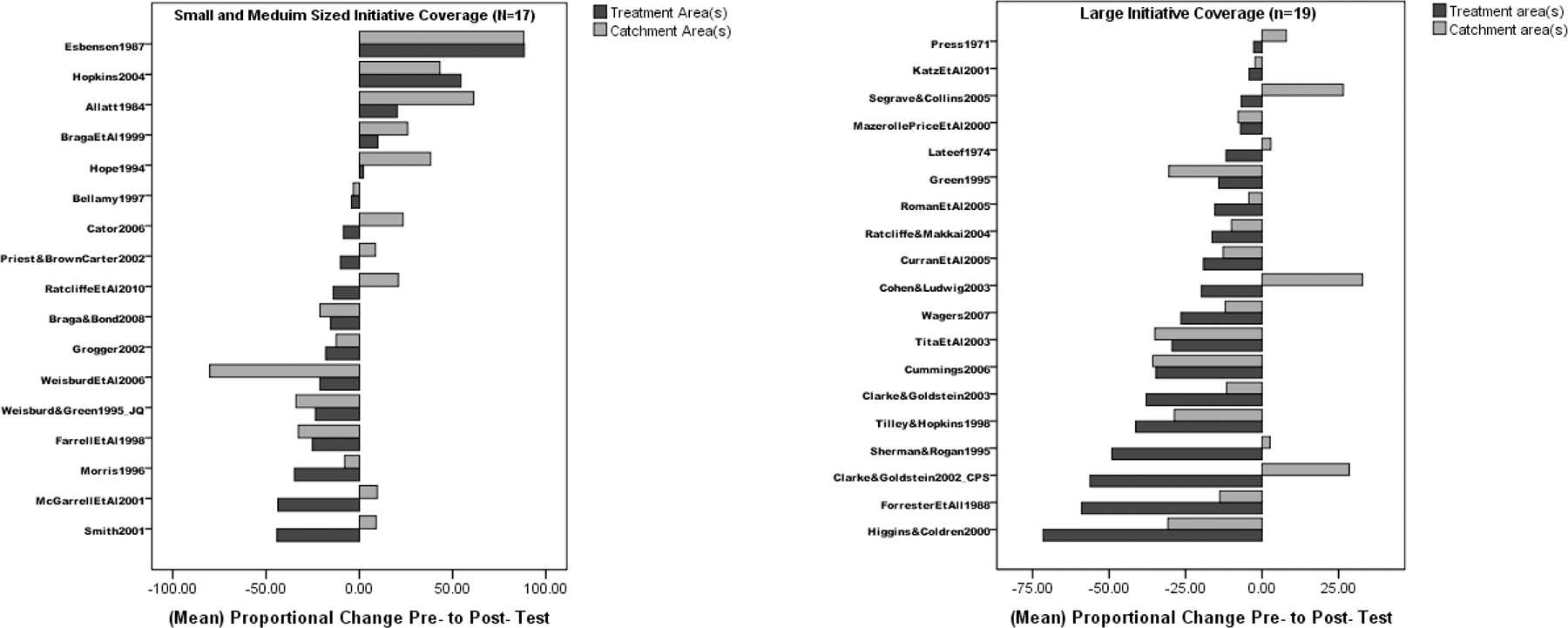
Proportional Change Pre to Post test for treatment and catchment areas by initiative coverage

5. Discussions and Conclusions

The aim of this review was to assess the degree to which geographically focused policing initiatives displace crime or diffuse crime control benefits to nearby areas. Hence it should be stressed here that these results are for a particular subset of crime prevention initiatives; those for which local level displacement and diffusion effects were examined. In choosing a fairly broad definition of ‘focused policing initiatives’ (including for example hotspots policing, POP, police patrols and crackdowns, broken windows policing and civil injunctions) our intention was to be able to make statements about focused policing efforts more generally. The number of studies that met our criteria was respectable at N = 44. Furthermore, there was a reasonable subset (n=16) that we were able to include in our meta-analysis section.

The main findings of the meta-analysis suggested that on average geographically focused policing initiatives for which data were available were (1) associated with significant reductions in crime and/or disorder and that (2) overall, changes in catchment areas were non-significant but there was a trend in favour of a diffusion of benefit. To assess the effects of study design, intervention size and intervention type, subsets of the data were considered in separate analyses. For those studies with the highest level of methodological adequacy (RCTs), there was evidence of a treatment effect and significant diffusion of benefit. For the quasi-experimental designs, when the analysis focused on that subset of observations for which a treatment effect was observed, an apparently reliable diffusion of benefit was also noted. For studies where data was collected for a catchment control area as well as a treatment control area it was evident that using a different control area can ultimately influence the results and therefore it is advisable to collect data for control catchment areas where possible. The results suggest little difference in the conclusions for those interventions which vary in the size of the area over which they are implemented. Finally, schemes which relied on a problem-oriented policing framework appear to have a slightly higher association with a diffusion of benefit than do schemes that rely on intensive policing alone, although these differences were not statistically significant. Possible publication bias was addressed using the trim and fill procedure and concluded that any unpublished studies were unlikely to have a large effect on the conclusions given here.

The total net effect and weighted displacement quotient analyses offer further ways of assessing outcomes, but the overall conclusions from these analyses are the same as those summarized above. That is, for the studies included in the analysis, the weight of the evidence suggests that where changes are observed in catchment areas that exceed those that might be expected in the absence of an intervention, a diffusion of crime control benefit rather than displacement appears to be the more likely outcome.

The proportional analysis was conducted using the 36 studies for which pre- and post-intervention data were available for at least two areas; a treatment and a suitable catchment area. The results suggest that the majority of eligible studies experienced a decrease in crime in the treatment area indicating possible success of the scheme. The majority also experienced a decrease in the catchment areas suggesting the possibility of a diffusion of benefit. Again, these findings are consistent with all others reported here.

These findings, taken together with results from other reviews of displacement and diffusion, offer two primary implications for criminological theory. First, because diffusion of benefits was observed somewhat more readily than displacement among the studies examined, it suggests that offenders actively engage in situational reasoning and rationality, which is a primary assertion of the rational choice perspective. Were offenders compelled in their disposition to offend, less diffusion and more displacement would have been expected or at least reductions in the targeted areas would not have been found. This implies that crime behavior may be more “normal,” in the sense that it is driven by satisfaction of fundamental needs and wants which are guided by cognitive reasoning, rather than by sociological or psychologically entrenched deviant “propensities” (i.e. determinism).

It is possible that since the evaluations reviewed here entailed focused police action that some incapacitation effect may be responsible for both the observed reductions in the targeted areas as well as the tendency toward diffusion (i.e. since fewer offenders might have been on the street). If so, this would discount the evidence in support of reasoning among offenders. Though the analyses performed in this review cannot rule out this incapacitation hypothesis, given the corroborating finding among evaluations of situational interventions (Guerette and Bowers, 2009) which largely did not rely on incapacitation, this scenario seems less likely. It is also worth noting that it is unlikely that the focused policing operations resulted in the capture of all offenders during the course of the intervention which means some would have remained on the street to continue offending. Thus, if the remainder were compelled by disposition to offend, the patterns of crime reduction in the intervention areas or at least the diffusion effects in the catchment areas would have been less pronounced.

Second, the findings also provide continued support for the notion that crime opportunity is discontinuous rather than constant. This supports the routine activity perspective and the tendency of opportunity heterogeneity has been implied in a succession of research (Brantingham and Brantingham, 1981; Eck, Clarke, and Guerette, 2007; Pease, 1998; Sherman, Gartin, and Buerger, 1989). If crime opportunity were constant then much more displacement would be expected since offenders could easily go elsewhere to reap the rewards of crime. Instead, the evidence suggests that crime opportunity concentrates to such a degree that effort to prevent crime by elimination of the offending opportunities in those areas, whether that be through focused policing or situational alterations, stands as a formidable means of crime reduction.

As with any research, there are a number of caveats associated with the review and outstanding questions that could be usefully addressed. In the authors' view three areas of enquiry would be particularly useful. First is the methodological issue of how to analyze displacement at the individual initiative level. In the process of this review we found many different strategies for doing this; all with their own merits and drawbacks. One particular issue was that many authors consider changes in treatment, catchment and control areas independently, not relating changes in one type of area to those in another. This was evident for some studies that compared changes pre- and post-intervention and for some that used formal time-series models. In the future, it would be helpful if study authors also reported interaction terms to indicate if the changes observed in catchment areas exceed those observed in suitable control areas, above and beyond what might be expected as a result of sampling error.

Second is a consideration of the physical areas selected to assess displacement and diffusion of benefit. There was considerable variation in the selection of the catchment areas used across studies; and almost none considered the issue of directional displacement; the default being to consider changes in a concentric ‘ring’ around a treatment area. Third is further investigation into the role of context and mechanism with regard to displacement and diffusion of crime control benefit. It is likely that the degree to which displacement and/or diffusion occurs will depend on a broad range of different factors including:

The effectiveness of the policing activity in reducing crime

The type of policing intervention

The type of crime that is the focus of the intervention

The intensity and effectiveness of implementation

The physical and social context of the scheme

The perceptions and motivations of offenders in the area

The context of the catchment area

Further investigation of these mediating factors would be useful in alerting practitioners to the conditions in which displacement is more or less likely.

In summary, the message from this review is a positive one to those involved in the sort of operational policing initiatives that were considered here. The main point being that displacement is far from inevitable as a result of such endeavors, and, in fact that the opposite, a diffusion of crime control benefits, appears to be the more likely consequence.

6. Plans for Updating the Review

The authors expect to update this review every five (5) years.

7. Statement Concerning Conflicts of Interest

Kate Bowers and Rob Guerette are the study authors of the most recent systematic review of crime displacement and diffusion of benefits among situational crime prevention interventions. Kate Bowers and Shane Johnson developed (with later elaboration by Eck and Johnson) some of the statistical procedures proposed to be used in this review. Bowers, Johnson, and Guerette have all published in the areas of problem-oriented policing, situational crime prevention, and environmental criminology. Guerette is affiliated with the Center for Problem-Oriented Policing and all (Bowers, Johnson, and Guerette) have written series guides commissioned by that organization. Guerette also serves as the advisor and coordinator for the annual Herman Goldstein Awards for Excellence in Problem-Oriented Policing.

8. Acknowledgments (in alphabetical order)

Anthony Braga, John Eck, David Farrington, Charlotte Gill, Elizabeth Groff, Lorraine Mazerolle, David McClure, Jerry Ratcliffe, Rachel Tuffin, Brandon Welsh, David Weisburd, David Wilson. Particular thanks to David Wilson and David Weisburd for their suggestions regarding methodology. Thank you also to all those involved in the review process, whose comments have been very helpful.

Footnotes

Appendix A

Appendix B

Appendix C

Appendix D

Appendix E

Appendix F

Appendix G

4

This section was adapted from .

5

Though offender displacement is often mentioned as a sixth type it is more accurate to describe this as offender replacement since it entails new offenders taking the place of other offenders who have been arrested or who have desisted from crime. Thus, it is not a form of displacement, which is a term reserved for changes that original offenders make so they can continue to offend when faced with reduced opportunities.

6

For more on this see .

7

The first to note this was where she writes, “Displacement is always a possibility, and while the displacement of crime through a planning intervention has target-specific value, it has no overall value unless it takes the form of displacement from more serious forms of criminal behavior to a less serious form.”

8

Another interpretation of deterministic theories, however, might contend that because offenders maintain some deep seated compulsion to commit crime they would be insensitive to the implementation of crime prevention schemes and would continue to offend in those areas targeted until incapacitated. Thus, displacement would not be predicted under this interpretation since offenders would be viewed as not possessing the capacity to make reasoned decisions as to when and where to offend in order to escape detection. However, this understanding may be overly reductionist since even committed dispositional theorists would recognize that situations play some part in crime, even if minor (for instance, see Sutherland, 1947, as noted by Weisburd et al., 2006:552).

9

One caveat is that did report on observed diffusion effects in 6 of the 55 studies reviewed as reported herein.

10

Note that in this case all the studies that were found meeting the criteria were written in English.

11

These publications were chosen because these journals in particular frequently publish evaluations of crime prevention interventions. Evaluation studies are sent to these locations as they are seen as the more applied journals in the field. The Home Office and the AIC do not have particularly comprehensive search engines.

12

By this we mean a trial in which the treatment and control conditions are randomly assigned to the participants. This is also termed as ‘random allocation’ or Randomized Controlled Trials (RCTs). We use these terms interchangeably in this review.

13

These areas are defined in the section below

14

There are existing scripts for performing meta-analysis (see ). These were not used in this analysis as the permutation method used here was not a standard approach and required programming.

15

Please note that for time series studies the data was processed so that it was possible to calculate a single odds ratio which compared the crime count across the entire pre- period to that of the entire post- period. Hence, a single area time series study would glean only one effect size.

16

It should be noted of course, that the results of these permutations will always be contained within the range for the worst-case to the best-case scenarios.

17

In the word buffer is used rather than catchment, but we use the latter here for consistency with vocabulary used throughout this report.

18

These sizes were inductively determined by noting from the studies the geographical scope of the intervention. Across the studies reviewed size of intervention area information was conveyed in a number of different ways, such as population, physical extent, or administrative boundary. Once collected relative categories of small, medium, and large geographical areas were partitioned. Small intervention areas ranged from one (1) household to 5 blocks in size; Medium intervention areas ranged from the area of a single housing estate up to comparable areas equivalent to about three (3) square miles; Large intervention areas were those that involved a scheme that covered any geographical area larger than 3 square miles. Note that because studies reported intervention area size in different ways, some subjective determinations were made by the authors. Specific details of each study are given in the narrative summaries in Appendix B.

19

The proportional change analysis simply quantifies change in the treatment and catchment areas without considering changes in control areas. See section 4.6

20

For a fixed effect model the weighted mean OR was 1.11 (CI: 1.05-1.18).

21

In the analyses that follow we consistently report 95% confidence intervals unless there are too few permutations for this to be meaningful. For example, where there are (say) only eight permutations we report the highest and lowest values rather than using confidence intervals.

22

As the random effects model is more conservative we use that in both cases. However, identical conclusions emerge for the fixed effects model.

23

The study was removed from this analysis because while the authors examined a series outcomes in this study, data for the catchment areas were only available for the scenario where the treatment effect was most positive.

24

Weighted mean effect sizes calculated using a random effects model are shown for the purposes of illustration only.

25

The alert reader will notice that while the weighted mean effect size for the best case scenario was marginally non-significant, three of the eight weighted mean effect sizes shown in were statistically significant. This illustrates the value of adopting the permutation approach as a safeguard. To elaborate, the identification of the best case scenario based on the point estimates of effect size does not account for the variance associated with those estimates, whereas the permutation approach does.