
Abstract
Using an environmentally extended social accounting matrix as well as a computable general equilibrium model, this study gauges the economic and environmental impact of Australian carbon tax, with an emphasis on the tourism industry. The results of the simulation show that a carbon tax of US$23 per tonne is very effective in achieving emissions reduction but also causes a mild economic contraction. Although the nominal value of tourism expenditure registers an insignificantly positive growth as a consequence of the carbon tax, the real expenditure value shows a significant decline in both inbound and domestic tourism demand. The household compensation package stimulates domestic tourism considerably but discourages inbound tourism further by contributing to a significant appreciation of the Australian dollar.
Introduction
The tourism industry contributes substantially to the Australian economy, albeit tourism as a share of the economy has declined in recent years. The Australian tourism satellite account showed that, with US$23.7 billion inbound tourism revenue in 2010–2011, tourism accounted for 9.0% of total services exports and remained as Australia’s No. 1 services export industry (Australian Bureau of Statistics, 2011). However, the growth rate of international tourist arrivals to Australia slowed down considerably over the period from 1990 to 2009. The annual growth rate averaged only 0.7% over the period 2000–2009, while the annual growth rate was 9.1% on average during the 1990s. According to Tourism Research Australia (2013), the tourism industry contributed US$41.1 billion directly and US$46.2 billion indirectly to national gross domestic products (GDPs) in 2011–2012. The total tourism contribution of US$87.3 billion accounted for 5.9% of GDP. This contribution presents a 2.4% decline compared to the peak tourism contribution to GDP of 8.3% in 2000–2001. In recent years, the tourism industry has underperformed in comparison to the broader economy. During the period from 1997–1998 to 2011–2012, the total tourism GDP increased at an average rate of 4.6% per annum, while the Australian GDP increased at about 6.8% per annum.
The introduction of carbon pricing in Australia – The Clean Energy Bill in 2011 – has triggered serious concerns in various tourism-related sectors. In May 2011, the Tourism & Transport Forum (TTF) expressed its support for a carbon tax but also expressed serious concerns about the carbon-tax-induced job losses, rising costs and the uneven playing field in competing with tourism industries in other countries (TTF, 2011). TTF estimated the carbon tax would cause a loss of tourism revenue of between 0.7% and 1.2%, a loss of net profit of up to 10% and job losses of between 3600 and 6400. TTF suggested a number of complementary measures to reduce carbon emissions in the industry and pleaded for government transitional assistance to the tourism industry. According to one of major Australia’s newspapers – The Australian, Col McKenzie from the Association of Marine Park Tourism Operators expected the cost of marine diesel fuel to rise by 6 cent a litre under a carbon tax. He said ‘for one of our big operators, that’s an additional (cost of) $270,000 a year, with no additional profits and no compensation. Tourism is already on its knees and we’re in diabolical trouble, looking at a cost like that’ (The Australian, 2011). Tourism Accommodation Australia (TAA) subsequently commissioned AECgroup to research into ‘the impact of the carbon tax on Australia’s accommodation industry’. Based on the research report, the TAA concluded that: TAA’s concerns continue to grow regarding Australia’s recent introduction of a carbon tax. Carbon pricing is impacting heavily on accommodation businesses, with profit reductions of up to 12% attributable to increased costs related to the tax. It is estimated that across the Australian accommodation industry the carbon tax cost will be up to $114.9 million in its first year. (TAA, 2013)
The negative impact of a carbon tax on tourism sectors is easily understood because of the contractionary nature of carbon pricing. However, to what degree will the tourism sectors be affected by a carbon tax? Should the tourism industry support or fear a carbon price? What kind of complementary policy is needed when a carbon price is in place? To answer these questions, comprehensive economic modelling is required. To quantify the effects of the Australian carbon tax, we developed a single-country, comparative static computable general equilibrium (CGE) model. An environmentally extended micro social accounting matrix (SAM) was also constructed. By analysing the simulation results, we endeavour to uncover the impact of the Australian carbon tax policy on the tourism industry.
The motivation of this study needs to be justified, given the political development in Australia. Although the Australian carbon tax was repealed by the new liberal government in 2014, it is still important to study the impact of a carbon pricing policy. Because the global warming and thus carbon emission issues will not go away, a carbon pricing policy will come to the government attention in Australia or in other countries. For example, the top carbon emitters including China and United States are taking action to address carbon emission issue. In Australia, the government agrees to start an emission trading scheme if the world major emitters have a price on carbon emission. Another evidence of the importance of a carbon price is the 2014 Climate summit in New York, which generated unprecedented worldwide marches, calling for actions on climate change.
The paper is organized as follows. The studies on the Australian carbon tax policy and on the impact of carbon pricing on tourism are reviewed in the previous empirical studies section. The model structure and database used for the simulations are described in the model and data section. The simulation results are presented and discussed in the simulation results section, with special reference to the tourism sectors. The final section summarizes and comments on the results.
Previous empirical studies
There are a large number of studies on carbon dioxide emissions. Notable publications include Beausejour et al. (1992), Devarajan et al. (2011), Hamilton and Cameron (1994), Labandeira et al. (2004), Wissema and Dellink (2007) and Zhang (1998). Due to space limitations, we confine our review of CGE modelling to Australian carbon tax policies and to studies of the impact of carbon pricing on tourism.
To implement a carbon tax in Australian, The Treasury (2011) carried out very complex large-scale carbon price modelling. This work consisted of a number of models, but the primary model for the Australian economy was the Monash Multi-Regional Forecasting (MMRF) model, which projected the national, regional and sectoral impacts of carbon tax. The modelling framework and results were included in a treasury report (The Treasury, 2011) and more recently in a book chapter on environmental CGE modelling in Australia by Adams and Parmenter (2013). Moreover, Meng et al. (2013a) developed a 35-sector (commodity) CGE model and simulated the effects of the Australian carbon tax on both the environment and the economy. The study suggested that the Australian carbon tax would cut emissions significantly at the price of a mild economic contraction. Although nominal GDP and gross national product (GNP) both demonstrated substantial growth in the carbon-tax-only scenario, the economy contracted mildly when real GDP and real GNP were used as measurements. However, real GNP registered significant positive growth under a carbon-tax-plus-household-compensation policy. On the return to the primary factors, the return on capital and on land decreased substantially in both scenarios. The return on labour reduced only slightly under the carbon-tax-only scenario, and increased significantly when a household compensation policy was in place. In the absence of household compensation, the internal balance improved substantially. Even with household compensation, the increase in government revenue was greater than the increase in its expenditures. Household consumption decreased slightly in the carbon-tax-only scenario but increased significantly when household compensation was included. Importers were found to benefit marginally under the carbon-tax-only scenario and to benefit significantly in the carbon-tax-plus-household-compensation scenario. In contrast, exporters fared badly, with an almost 3% drop in real exports under the carbon-tax-only scenario, and a more than 6% drop under the carbon-tax-plus-household-compensation scenario.
There are a number of studies on the impact of carbon pricing on tourism, including AECgroup (2013), Blanc and Winchester (2013), Dwyer et al. (2012, 2013), Mayor and Tol (2007, 2010), and Tol (2007). We review them briefly here.
Using a model based on domestic and international tourist flows, Tol (2007) estimated the implication of imposing an emission tax on aviation fuel. The study found that the effect of tax on travel behaviour would be small because the imposed tax was small relative to the airfare. A global US$1000 per tonne emission tax on aviation fuel would reduce travel behaviour to the extent that international aviation carbon emissions could decrease by only 0.8%. The emission tax on aviation fuel would have a more notable impact on long-haul and short-haul flights, with medium distance flights being less affected. If the emission tax was applied only to the European Union (EU), tourism within the EU would grow at the price of a decrease in tourism arrivals in other relatively remote tourist destinations. The rationale was that EU tourists would stay closer to home under the emission tax.
Also based on the domestic and international tourist flows, Mayor and Tol (2007, 2010) estimated the impact of carbon pricing policy in the United Kingdom and, more generally, in the EU. Mayor and Tol (2007) studied the UK’s proposed changes in the air passenger duty (APD). They found that the doubling the APD would surprisingly cause a slight rise in carbon dioxide emissions. Tourists travelling to the United Kingdom would fall slightly, tourists travelling from the United Kingdom to destinations near United Kingdom would also fall, but tourists leaving the United Kingdom for destinations further afield would increase. It was also found that the proposal of the Conservative Party to exempt the first 2000 miles (for UK residents) would decrease emissions by the amount similar to that of abolishing the APD altogether. Mayor and Tol (2010) investigated the effect of various climate policy instruments implemented in Europe. They claimed that introducing aviation into the European carbon trading system would discourage tourists travelling into the EU, caused a significant welfare loss while achieving a small amount of emissions reduction. Similarly, imposing flight taxes in the Netherlands and the United Kingdom was found to reduce visitor numbers to these countries and also induce global welfare losses.
Blanc and Winchester (2013) estimated the additional costs to airlines due to the EU Emissions Trading System (ETS) on travel to 26 Caribbean destinations. The study used a downward sloping demand function for air transportation services to generate the changes in tourism arrivals and in airfares. With a proposed EU emission allowance price of €10, it was estimated that there is an average cost increase of US$17 for a round trip from Europe to the Caribbean by indirect flights. For direct flights, the cost increase is averaged at US$21. These additional costs were found to reduce tourism from the EU to the Caribbean by between 1.4% and 2%, and reduce total tourists arrivals to the Caribbean by less than 0.4%.
In Australia, Dwyer et al. (2012, 2013) used a dynamic CGE model MMRF-green and data from the Australian tourism satellite account to assess the potential economic impact of the Australian carbon tax on the tourism industry. They found that, compared with the baseline case, domestic tourism consumption would change by −0.63% in 2015 and −1.17% in 2020, while for international tourism consumption the change would be −0.265% in 2015 and −2.47% in 2020. They also found that, compared with the projected baseline values over the period to 2020, most tourism industries in Australia would experience a mild contraction in output as a result (−0.02% to −1.48%). This contraction is in line with the slowing down of the economy as a whole. The reduction in tourism employment was found to be slightly larger than in other Australian industries. The largest associated falls occurred in accommodation, air and water transport and in the cafe, restaurant and food outlet industries.
The research by AECgroup (2013) in Australia is relatively simple but worth mentioning because of the fear it caused within the tourism industry. The study is basically a production cost analysis. Based on the itemized estimations of carbon-tax-induced cost hike from various sources, the researchers proposed two scenarios: high-impact scenario and low-impact scenario. In the low-impact scenario, the cost of foodstuffs in preparing meals was estimated to increase by 0.4%; liquor and other beverages by 0.4%; electricity, gas and water charges by 10%; repair and maintenance by 1.5%; laundry and cleaning services by 3.0%; and land tax and land rates by 1.0%. In the high-impact scenarios, the cost increase for these items was 1.1%, 0.5%, 13.6%, 2.0%, 5.0% and 2.0%, respectively. Based on these estimates, the researchers calculated the total cost impact and the profitability impact to the accommodation industry. It was estimated that the total cost would increase by 0.5% or A$64.5 million in the low-impact scenario and by 0.9% or A$114.9 million in the high-impact scenario. This presents a reduction in profit margin by 6.6% in the low-impact scenario and 11.8% in the high-impact scenario.
In summary, there are a number of studies on the tourism impact of carbon pricing, but most of them only analyse the impact of particular tourism-related industries such as aviation and accommodation. More importantly, most adopted a partial equilibrium analysis framework, which has serious limitations as identified by previous studies (see Blake, 2000; Briassoulis, 1991; Dwyer et al., 2004). Dwyer et al. (2012, 2013), and Blanc and Winchester (2013) did employ a CGE model in their study, but there was no detailed tourism sector in their CGE model. In their study, the effect of carbon tax on tourism was estimated by linking the CGE model to a partial equilibrium model or to the tourism satellite account. This study developed a CGE model with detailed energy and tourism sectors and built an environmentally extended SAM. This study is based on the simulation results from this model.
Model and data
The CGE model used in this study is based on Meng et al. (2013a), which in turn was based on ORANI-G developed by Horridge (2000). In order to allow for the substitution between different fuel types and between energy and primary factors, and for the feedback effect of households’ responses to government policy, Meng et al. (2013a) significantly changed the production structure in ORANI-G and added a SAM extension in the model. For the purpose of this study, the model by Meng et al. (2013a) has also been modified considerably. The main changes include the aggregation of the multi-household group and tourism extension. In order to facilitate the reader’s understanding of the modelling results, we briefly describe the model structure, with an emphasis on the changes made for this study.
In the model, the Australian economy is represented by 42 sectors and 42 commodities (including 2 shadow tourism sectors), 1 representative investor, 1 government, 1 representative household and 9 occupation groups.
The production function consists of a multiple-level nested Leontief and Constant-Elasticity-of-Substitution (CES) function with great details about energy use and carbon emission generated. The intermediate inputs are divided into two groups: energy inputs and non-energy inputs. For energy inputs, CES functions are used at the bottom level to combine black coal and brown coal in order to form composite coal; oil and gas are combined to form composite oil–gas; and automobile petrol, kerosene, liquefied petroleum gas and other petrol are combined to form composite petroleum. At the second level, composite coal, oil–gas, petroleum and commercial electricity are combined by a CES function to form composite energy. At the third level, a CES function is used to combine composite energy with capital to form capital–energy composition. At the fourth level, a CES function is used to combine capital–energy composition, labour and land to form the primary factor; domestic goods and imported goods are combined to form composite non-energy intermediate inputs; and different electricity generations are combined to form composite electricity generation. At the fifth (or top) level, the primary factor, electricity generation and non-energy intermediate inputs are combined by a Leontief function to create the sectoral output.
There are three types of carbon emissions in the model: stationary emissions, activity emissions and consumption emissions. The stationary emissions refer to the emissions generated from combustion of fuels. This type of emissions is assumed to be proportional to the amount of fuels used, namely, the amount of the fuel multiplied the emission intensity of the fuel. The emission intensity of fuels is calculated based on the base year stationary emissions data and fuel inputs data for each industry and for each fuel type. The activity emissions refer to the emissions by each industry unable to attribute to fuel inputs, for example, fugitive emissions, process emissions and bush fire (for agricultural sector). This type of emissions is assumed to be proportional to the output of the industry, namely, the industry output multiplied by the output emission intensity. The output emission intensity is calculated using the base year data on output and activity emission for each industry. Consumption emissions refer to the emissions generated from households’ consumption. This type of emissions is assumed to be proportional to household consumption level. Again, the consumption emissions were obtained by multiplying the amount of household consumption by the consumption emission intensity coefficients, which were pre-calculated from the base year emission data and household consumption data. Since the short-run effect of a carbon price is the main concern of this study, the technology and household preferences are unlikely to change. Therefore, all three types of emission intensity are fixed in the model.
The household, investment, government and exports make up the final demand in the model. The functions for final demands are similar to those in the ORANI model (Dixon et al., 1982), for example, a nested Leontief-CES function for the investment demand and a nested Linear-Expenditure-System (LES) and CES function for household demand. However, unlike the assumption of exogenous total (or supernumerary) household consumption in ORANI-G, household consumption in this study can vary based on household income change. Since substantive (or necessity) consumption is unlikely to change in response to income changes, all changes in consumption largely stem from changes in supernumerary consumption. A Keynesian style consumption function is adopted, so supernumerary consumption is assumed to be proportional to total income which varies under the carbon tax policy. The multiple households in Meng et al. (2013a) were aggregated into a single household because no survey data were available on tourism expenditure by household income group.
Because the tourism industry is a demand-side concept, that is there is no concrete tourism industry in reality, the modelling of tourism is achieved by creating shadow tourism sectors. The spending pattern for inbound tourists is quite different from that of domestic tourists, so that these two groups of tourists are treated as independent tourism demands. In the model, two shadow tourism sectors – the inbound tourism sector and the domestic tourism sector – are created to cater to the responding tourism demands. This treatment of the tourism sector is similar to that in Pham and Dwyer (2013). That is, these two tourism sectors actually act as a middleman to buy goods and services from other sectors and then sell to tourists. One benefit of creating ‘shadow’ tourism sectors is that tourism expenditure will strictly follow the pattern shown by tourism surveys. The other benefit is that it is possible to generate aggregated results for the tourism industry such as sectoral output, employment, profitability, emission cuts and carbon tax burden. The difference of this approach is that it does not allow for the substitution effect (flexibility of choice) in tourism spending on different type of goods and services, which is allowed for in Meng et al. (2013b). The total inbound tourism expenditure is modelling in the traditional way – tourists respond to the changes in the prices of tourism goods and services and to changes in the exchange rate. Essentially, inbound tourists are assumed to face a downward sloping demand curve. However, the modelling of domestic tourism spending is achieved in an innovative way. The traditional way of modelling domestic tourism is the same as modelling inbound tourism – the price of tourism-related goods leads to variation in tourism expenditure. This approach ignores the important effect of the change in household income on domestic tourism expenditure. Utilizing the data in household accounts in SAM, this study allows total domestic tourism expenditure to respond to changes in household income while also allowing tourism expenditure to respond to changes in the price of tourism goods. This approach is important in the case of a household compensation package which increases household income substantially.
There are three main types of data for the modelling: input–output (I-O) data, carbon emission data and various behavioural parameters. The —I-O data used in this study come from the Australian Input–Output Tables 2004–2005 published by the Australian Bureau of Statistics (ABS, 2008). For the purpose of this study, the 109 sectors (and commodities) in the original I-O tables were disaggregated and aggregated (disaggregating the resources and tourism sectors and aggregating other sectors) to form 40 sectors (and commodities). Labour supply was disaggregated to nine occupation groups based on the household expenditure survey data published by the Australian Bureau of Statistics (ABS, 2006a). The carbon emissions data are obtained from the Greenhouse Gas Emission Inventory 2005 published by the former Department of Climate Change and Energy Efficiency of Australia. The data are called CO2-equivalent data, which include all greenhouse gas emissions with other greenhouse gas emissions converted to the equivalent amount of CO2. The tourism demand data are from the 2004to 2006 tourism satellite account (ABS, 2006b). Since the classifications in the tourism satellite account and in the I-O tables are not the same, the tourism demand data are mapped into the I-O tables.
The elasticity for tourism demand is a key parameter for this study. Kulendran and Divisekera (2006) estimated the elasticities of international tourism demand from the United States, Japan, United Kingdom, and New Zealand to Australia at 0.67, 0.45, 0.55, and 1.68, respectively. Divisekera (2007) estimated the domestic and international tourism demand in Australia. According to this study, the Marshallian price elasticities of domestic tourism demand for food, accommodation, transportation, shopping and entertainment were 0.910, 0.624, 0.505, 0.503 and 0.499, respectively. For international tourism demand, they were 0.837, 0.391, 0.282, 0.757 and 1.722, respectively. Based on these estimations, the elasticity of both inbound and domestic tourism demand is assigned a value of 0.6. Most of the other behavioural parameters in the model are adopted from ORANI-G, for example, the Armington elasticities, the primary factor substitution elasticity, the export demand elasticity and the elasticity between different types of labour. Since Australia is a small trading country and thus a price taker in most global commodity markets, export demand curves should be fairly flat, reflecting that export demands are very elastic. As a result, the export demand elasticity for most of the goods is given a large value (around 10). For the agricultural sectors, the elasticity values are even larger (around 12) to take into account the relatively small size of agriculture exports. However, Australia is a major supplier of natural resources, so the export elasticity for Australian natural resources is much smaller than that for other commodities. Consequently, smaller values are assigned for natural resources, for example, a value of 5 is used for the exportation of black coal.
The substitution effect between different electricity generations is assumed to be perfect because of the homogeneity of electricity, so a large value of 50 is assigned to their substitution elasticity. The substitution elasticity for other energy inputs are as follows: The energy inputs at the lower level, that is, between black and brown coal, between oil and gas, and between the various types of petroleum, have a relatively high similarity, so a value of 0.5 was assigned for the substitution elasticity among them. The composite energy inputs at the upper level, namely, between composite coal, oil and gas, petroleum and commercial electricity are less substitutable, so a value of 0.2 was assigned for the elasticity of composite energy inputs. The substitution effects between composite energy and capital are generally considered very small, so small elasticity values between 0.1 and 0.6 are commonly used in the literature. In this study, we assume the cost of energy-saving investment is very high, given the current technological situation, which is unlikely to change in the short run, and thus there is a very limited substitution effect between capital and composite energy. Consequently, a value of 0.2 was assigned for this substitution elasticity.
Simulation results
Since the purpose of this study is to estimate the impact of the Australian carbon tax policy on the tourism industry, the simulation shock is chosen to mimic the carbon tax proposed by previous labour government. Therefore, the carbon price is set at A$23 per tonne of carbon emissions (or US$23 per tonne because the Australian dollar was at parity with the US dollar in 2012), but the agriculture and household sectors are exempted from the tax. Accompanying the carbon tax, the government also proposed a compensation package, which is quite complicated. For example, manufacturers and exporters can get various levels of compensation. For households, the government changed income tax thresholds and provided various family tax benefits such as ‘clean energy advance’, ‘clean energy supplement’ and ‘single-income family supplement’. To mimic the compensation package would unnecessarily complicate this study. Therefore, only a simple revenue-neutral compensation was considered for households: All carbon tax revenue is transferred in lump sum to all households. To estimate the effects of both the carbon tax and the household compensation package, this study simulates and compares two scenarios: (a) US$23 carbon tax only and (b) US$23 carbon tax plus household compensation.
The carbon tax policy is subject to variation in the long run. It is abolished in 2014 but the government may introduce an ETS when major emitters in the world have a carbon price. In this context, a short-run simulation is the objective of this study and a short-run macroeconomic closure is assumed, for example, fixed real wages and capital stocks, free movement of labour but immobile capital between sectors. The exchange rate is set as endogenous to reflect the flexible exchange regime in Australia.
The aforementioned scenarios are simulated using GEMPACK 11.2 and sensitivity tests are performed using the systematic sensitivity analysis built into the software. Following accepted practice, the results are listed as percentage changes unless otherwise specified. All changes are in comparison with the baseline case – business as usual, that is, assuming no carbon tax policy. The sensitivity tests show that, overall, the simulation results are only mildly sensitive to the elasticity values used. However, the elasticity values for different types of fuels are moderately sensitive to the environmental results (i.e. emission reductions).
Macroeconomic and environmental effects
The macroeconomic and environmental results are shown in Table 1. Overall, the modelling results show that under both scenarios, carbon tax only and carbon tax plus household compensation, carbon emission cuts are significant, and the economy will be affected negatively but mildly.
Macroeconomic environment.
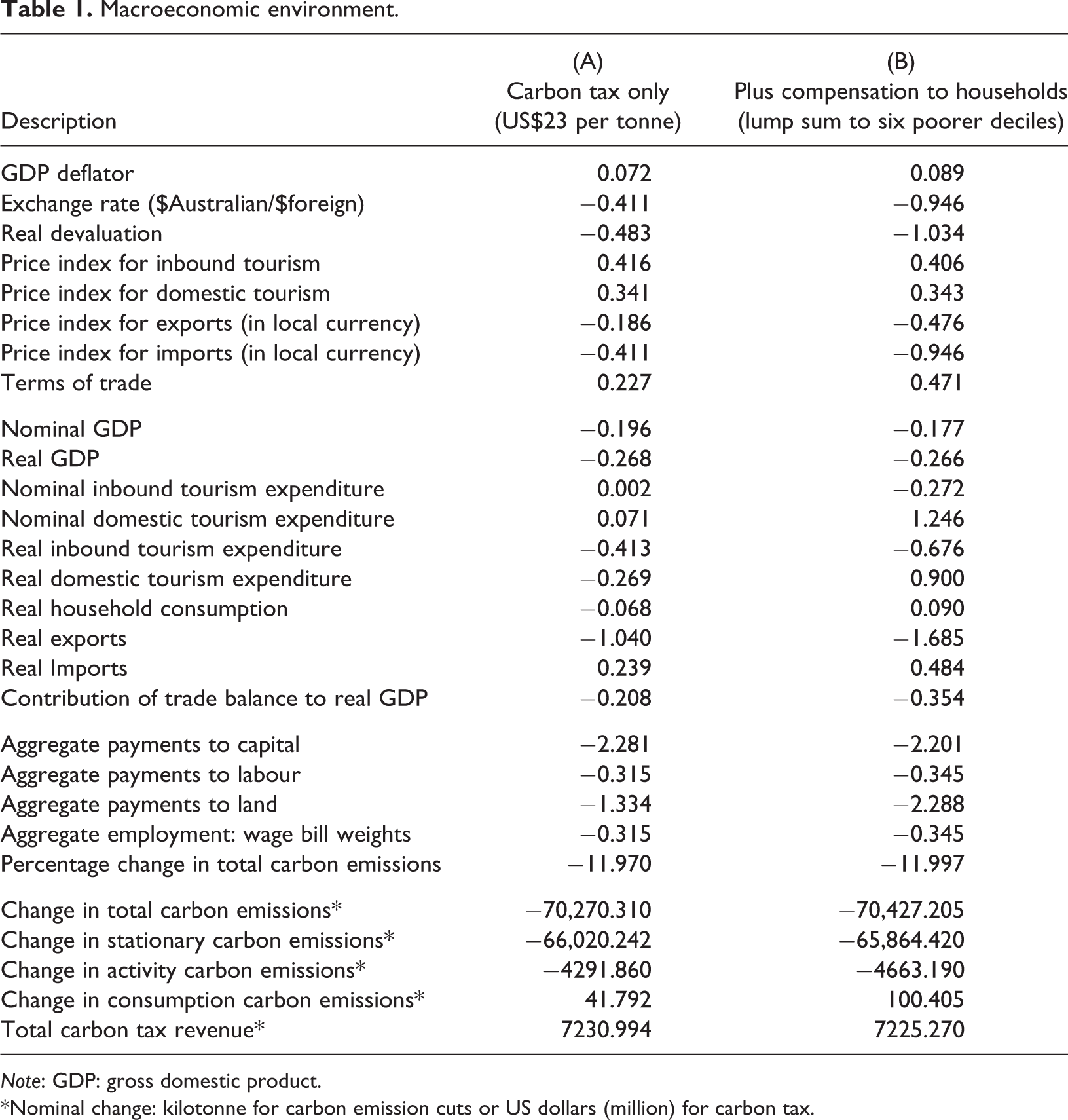
Note: GDP: gross domestic product.
*Nominal change: kilotonne for carbon emission cuts or US dollars (million) for carbon tax.
The first panel shows the changes in price level. Since Consumer Price Index (CPI) is used as a numeraire, the GDP price index (GDP deflator) acts as the indicator of the price level of the economy. The simulation results show that price increases only slightly (by 0.072% in scenario A and 0.089% in scenario B). However this is not the whole story because, under the flexible exchange rate regime, upward pressure on price level is also reflected in a more expensive Australian dollar. Including both the 0.411% decreases in the exchange rate (or appreciation of Australian currency) and the 0.072% increase in GDP price index in scenario A, the Australian dollar is overall inflated by 0.072% + 0.411% = 0.483%, indicated by a −0.483% real devaluation in Table 1.
The price indexes for tourism are much higher than the GDP deflator. This means that the carbon tax will more significantly affect the price of tourism-related goods, implying that these goods are relatively emission/energy-intensive compared with the broader GDP basket. The significantly higher prices of inbound tourism show that it is more emission intensive than domestic tourism. This is consistent with the fact that an inbound tourist will spend more on air transport and road transport than a domestic tourist. Compared with scenario A, the increase in inbound tourism price is slightly smaller in scenario B and that for domestic tourism price is marginally higher. This is consistent with lower inbound tourism demand and higher domestic tourism demand in scenario B than in scenario A, shown in the second panel of Table 1. Given the unchanged world price, the appreciation of the Australian dollar makes imports cheaper for Australians while exports become more expensive to foreigners. The higher prices faced by foreigners discourage export demand and thus lead to a decrease in export prices denominated in local currency. Since the decrease in price of exports is less than that of imports, Australia’s terms of trade improves by 0.227%.
The second panel displays the changes in GDP and its component on the expenditure side. Both nominal and real GDP decreases in all scenarios. Compared with the changes in nominal GDP, decreases in real GDP are significantly greater due to the positive GDP deflator in both scenarios. The decrease in real GDP is expected because a carbon tax increases production costs and thus discourages commodity supply. In the scenario B, real GDP decreased by less because the compensation policy stimulates household consumption and thus induces higher value adding than in scenario A.
In terms of nominal value, both inbound and domestic tourism expenditure in scenario A increase insignificantly. However, the results for real tourism expenditure show that both tourism demands decline significantly due to a considerable increase in tourism prices. Again, the decline in inbound tourism demand is much greater than the decline in domestic tourism demand. There may be two factors behind this. First, inbound tourism is more emission intensive and thus is subject to a greater price hike under a carbon tax. Second, inbound tourism suffers from appreciation of the Australian dollar in the wake of a carbon tax – that is, a stronger Australian dollar makes the costs faced by inbound tourists even higher and thus depresses inbound tourism demand. Both nominal and real expenditure on inbound tourism decrease further in scenario B than in scenario A while those on domestic tourism increase in scenario B. This is explained by the even stronger Australian dollar and the higher household income in scenario B where the household compensation package is implemented. The sizable growth in domestic tourism expenditure in scenario B demonstrates that the household compensation policy stimulates domestic tourism demand greatly.
Household consumption decreases in scenario A due to the higher prices and lower income resulting from the scaling back of production in the economy. However, compared with scenario A, household consumption in scenario B increases significantly, due to the lump sum compensation. The decrease in exports and increase in imports are the immediate effects of the appreciation of the Australian dollar: The more expensive Australian dollar means a higher price of Australian exports faced by foreigners and cheaper imports for Australians. The greater changes in imports and exports in scenario B than in scenario A are consistent with the further appreciation of the Australian dollar under the household compensation package. With a significant increase in real imports and considerable decrease in real exports, the contribution of trade balance to real GDP decreases remarkably.
The third panel shows the changes in aggregate employment and changes in aggregate payments to factors. The payments to capital decrease considerably in both scenarios. The decrease may stem from the fact that the decrease in demand for capital presses down the capital rental price. Compared with scenario A, aggregate payments to capital in scenario B improve. This is consistent with the improved GDP and household consumption in scenario B. Aggregate payments to labour decrease significantly in both scenarios. The further decrease in payments to labour in scenario B is somewhat perplexing, considering the smaller GDP decrease in scenario B than in scenario A. However, the result is not difficult to comprehend when the international trade effect is taken into account. The further appreciation of the Australian dollar in scenario B depresses Australian exports. Many export-oriented industries (e.g. agriculture, mining and manufacturing) are labour intensive. As these industries contract further in scenario B, it is of no surprise that the payments to labour will likewise decrease further. Aggregate employment changes at the same pace as aggregate payments to labour. This is due to the assumptions used in the simulation. The real wage is assumed to be unchanged in the short run and the nominal wage is fully indexed with CPI, which is fixed under the flexible exchange rate regime, so that changes in the total wage bill (payments to labour) is solely determined by changes in employment. Aggregate payments to land decreases less than aggregate payments to capital. It is easy to comprehend this because land is mainly used by the agricultural sector, which is less affected by the carbon tax due to the government’s exemption of the agriculture sector from the tax.
The last panel in Table 1 shows the carbon emission reduction and carbon tax revenue under two scenarios. The results show that US$23 per tonne carbon tax is quite effective, reducing carbon emissions by 70.270 megatonnes, or 11.970% of the emission base under the carbon-tax-only scenario. Under the household-compensation-package scenario, emission cuts are slightly greater. This comes as a surprise. It could be assumed that a lump sum money transfer to households would encourage consumption of all kinds of goods, including emission-intensive goods. As a result, carbon emissions should be greater compared with the no compensation scenario. However, this reasoning is correct only for a closed economy. Since the Australian economy represented in the model is an open economy with flexible exchange rate, the household compensation policy will lead to a significant appreciation of the Australian dollar and thus depress exports. As the decrease in exports outweighs the increase in domestic sales, the total output of the economy will decrease, leading to greater emission cuts in scenario B. The results of changes in different types of emissions confirm this reasoning. Compared with scenario A, stationary emissions and consumption emissions decrease further or increase more in scenario B, due to the increase in household consumption. However, activity emissions decrease more significantly in scenario B, leading to a further decrease in total emissions. The carbon tax revenue is calculated as the remaining emission base multiplied by the carbon tax rate of US$23, and the more than US$7 billion tax revenue implies a large amount of emissions remaining in Australia. The lower carbon tax revenue in scenario B is consistent with the greater emission reduction under this scenario.
Sectoral effects
In this section, we discuss the sectoral impact of the carbon tax through sectoral output, employment, and profitability, as shown in Table 2. Since tourism is the focus of this study, the tourism-related industries (where tourist purchase goods and services come directly from) are listed in the first panel. The results on the two aggregate or shadow tourism industries are displayed at the end of this panel. Due to the significant role of energy and resource industries in emissions reduction, the results for these industries are shown in the second panel. The remaining sectors are listed into the third panel.
Sectoral output, employment and profitability.
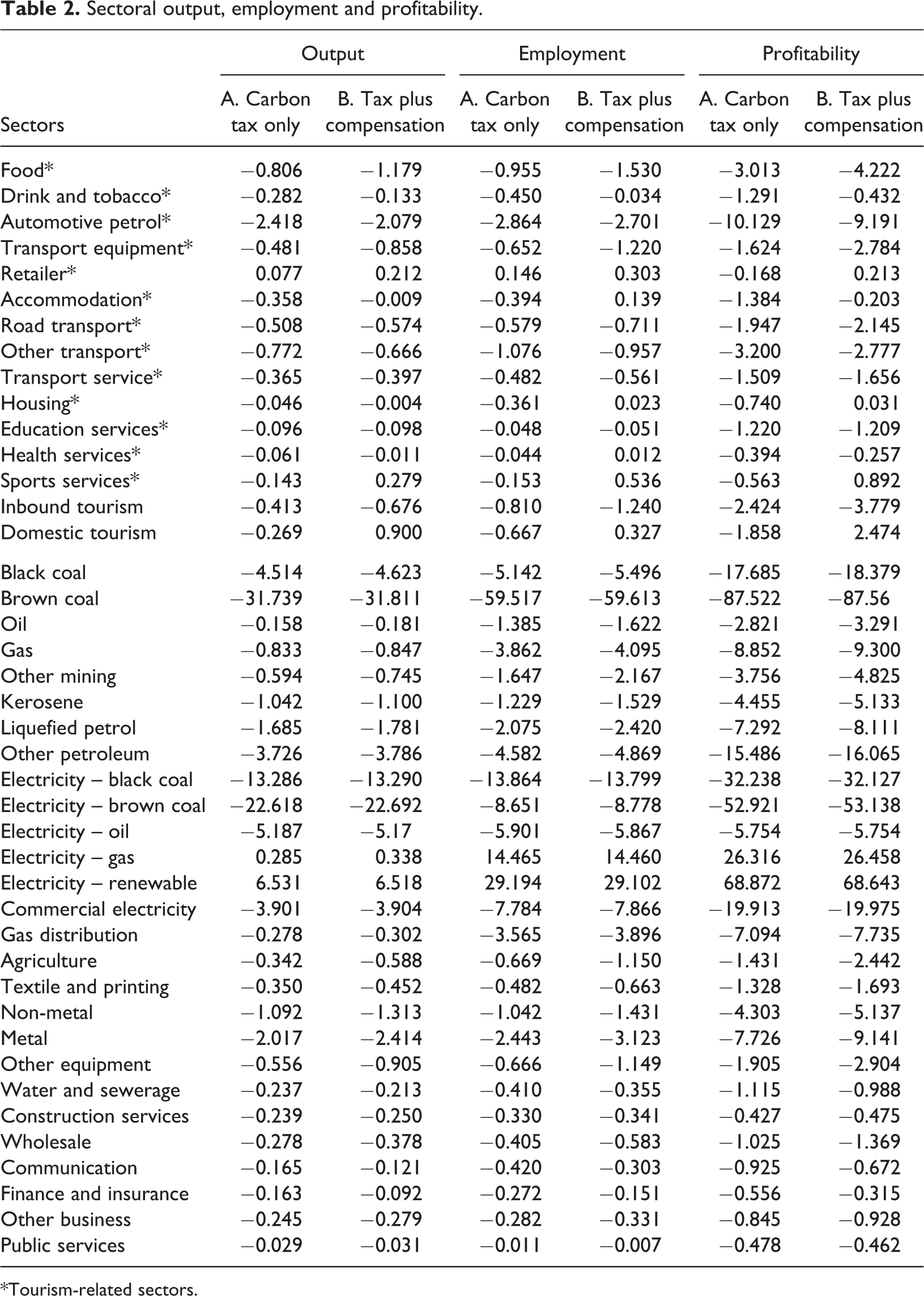
*Tourism-related sectors.
First, we discuss the changes in sectoral output in each panel. The impact of the carbon tax on tourism-related sectors varies considerably and largely depends on the emissions intensity of the sector. The largest decrease in output occurs in the automotive petrol industry. Due to its high emissions intensity relative to other tourism-related industries, this industry is hit hard by the carbon tax, indicated by a more than 2% decrease in sectoral output in both scenarios. The second group includes sectors such as food, transport equipment, road transport and other transport. These sectors are also emissions intensive, and the carbon tax will lead to a decrease in output of between 0.481% and 0.806%. The third group includes the drink and tobacco, accommodation, transport services, housing, education services, health services and sports services sectors. Output decreases for these sectors range from 0.046% to 0.365%. The last tourism-related sector to be discussed is the retail sector. Unexpectedly, the output of this sector increases by 0.077% in scenario A and by 0.212% in scenario B. Retail sector output increases in the wake of a carbon tax may indicate changed consumption patterns induced by the carbon tax; that is, as the prices of emissions-intensive goods increase substantially, the households may consume more goods of less emissions intensity such as retail services. The aggregated impact on tourism is significant: 0.413% decrease in inbound tourism and 0.269% decrease in domestic tourism under scenario A. The impacts of the household compensation policy on the tourism-related sectors shown in scenario B are mixed. For sectors like drink and tobacco, automotive petrol, retail, accommodation, other transport, housing, education services, health services and sports services, the output decreases less or increases more in scenario B than in scenario A, so these sectors benefit from the household compensation package. However, other tourism-related sectors will experience an additional output reduction in scenario B. The overall effects of the household compensation policy on the aggregated tourism sectors are also mixed: The policy will depress inbound tourism significantly but will promote domestic tourism greatly. This is explained by the increase in household consumption and by further appreciation of the Australian dollar in scenario B.
Second, we turn our attention to sectoral employment. The changes in employment shown in Table 2 have the same sign as the changes in output, but the magnitude of change is generally larger. The energy and resource sectors experience large changes in employment. The impact on the majority of tourism-related sectors is rather mild. With the exception of a 2.8% reduction in employment in automotive petrol sector and about 1% in the other transport sector, the decrease in employment in other tourism-related sectors is less than 1%. Overall, in the inbound tourism industry, there will be a 0.8% increase in unemployment in scenario A and 1.2% in scenario B. The domestic tourism industry will reduce employment by 0.7% in scenario A but will increase employment by 0.3% in scenario B. With the exception of non-metal and metal manufacturing, which experience decreases in employment by 1.04% and 2.44%, respectively, the employment effect on the other sectors listed in the third panel is also mild.
Last, we consider profitability. Due to the assumption of perfect competition in the model, the economic profit for each sector is zero, that is, all value added goes to returns to capital, land and labour. Profitability in this study is defined as the rate of return to capital, which is calculated as capital rental prices multiplied by the amount of capital employed in the sector. The changes in profitability in Table 2 follow the same signs as output and employment, but the degree of change is the highest. For the energy and resource sectors, the change in profitability is remarkable. The profitability of the brown coal sector decreases by over 87%. With the exception of automotive petrol, which experiences a 10% decrease in profitability, the decrease in profitability for tourism-related sectors is mild, ranging from 0.56% to 3.20%. The overall result for inbound tourism is a decrease in profitability of 2.45% in scenario A and 3.78% in scenario B. For domestic tourism, it is a decrease of 1.86% in scenario A but an increase of 2.47% in scenario B. For sectors in the third panel, the decrease in profitability is very mild (around 1%) with the exception of non-metal and metal manufacturing which experience 4.3% and 7.7% decreases in profitability, respectively. Comparing scenario A with B, we find that the household compensation package does more harm than good to most sectors, mainly because it results in depressed export demand and the changed consumption pattern in scenario B.
Conclusion
This study employed a CGE model and an environmentally extended SAM to simulate the impact of the Australian carbon tax, with an emphasis on the tourism industry. Generally, the modelling results show that the carbon tax can lead to significant cuts in carbon emissions while causing a mild economic contraction. The impact of the carbon tax on tourism is mild. Real inbound tourism expenditure will decrease by 0.413%, while domestic tourism expenditure decreases by 0.269%. The prices of tourism goods will increase by 0.416% for inbound tourism and 0.341% for domestic tourism. The decrease in tourism demand comes not only from an increase in operation cost but also from a more expensive Australian dollar for international tourism demand and from the reduced household income for domestic tourism demand. Among all tourism-related sectors, the food, automotive petrol, accommodation, road transport, other transport and transport services sectors will be affected significantly, indicated by a 0.358–2.418% decrease in output, a 0.482–2.864% decrease in employment and a 1.384–10.129% decrease in profitability. The retailer sector grows in the wake of a carbon tax, while the other tourism sectors are affected negatively but marginally. The emission reductions and carbon tax burdens on tourism sectors are largely in line with their emission intensities, so that transport-related (also tourism-related) industries play a significant role. The household compensation policy is found to have a significant negative impact on inbound tourism but can stimulate domestic tourism demand considerably.
The results of this study are in the middle range of estimations by other studies. Although international comparison is difficult due to different conditions in different countries, the following examples provide the significance of the estimates. Mayor and Tol (2007) estimated only a 0.02% decrease in tourism arrivals when the APD of United Kingdom doubles from 5.5 pounds for flights from United Kingdom to other European economic area, or from 22 pounds for other flights. Tol (2007) estimated a 0.8% decrease in international tourism arrivals when a US$1000 per tonne kerosene tax is imposed. These results show very insignificant impact of an emission-related tax. On the other hand, the study of Blanc and Winchester (2013) concluded that, assuming a carbon price of 10 euro (or US$13.24) for EU ETS and a unit elasticity of tourism demand, the EU tourism arrivals will decrease by 1.4–2.4% for direct flights and by 1–2.2% for indirect flights. These estimates are very significant. It should be mentioned that Blanc and Winchester (2013) used a partial equilibrium approach and assumed that the cost of carbon pricing will be fully passed on to tourists. This tends to generate a larger decrease in tourism arrivals.
In comparison with the Australian studies, the results of this study are similar to those by Dwyer et al. (2012, 2013). The overall impact on tourism expenditure in this study is smaller compared with a decrease in tourism consumption by 0.63% in 2015 and by 1.17% in 2020 in Dwyer et al. (2013). The difference between the two studies may be due to the different methods used. Since there is no tourism consumption in the MMRF-green, the tourism consumption in Dwyer et al. (2013) is estimated through the changes in output of tourism-related industry times the multiplier from the tourism satellite account. This does not take into account the feedback effect and thus tends to exaggerate the changes. On sectoral results, this study has wider range of change, for example, the output of tourism-related sectors change by −2.418% to 0.077% compared with −1.48% to 0.36% in Dwyer et al. (2013). Again, these may be due to the different method used. In this study, the output changes of tourism sectors are directly generated from the CGE model, so the results are underpinned by the sectors’ emission intensity and energy intensity. In Dwyer et al. (2013), the detailed tourism sector results are extrapolated from the results of MMRF-green, based on proposed ratios. These ratios may not precisely reflect the impact of the sectors’ emission intensity and energy intensity.
The modelling results have important implications for tourism industry. Since the tourism impact of the carbon tax is generally negative, it is understandable that the sectors either oppose the carbon tax or plead for subsidies. However, the negative impact is generally mild except for a few tourism sectors with high emission intensity. Compared with non-tourism sectors, this impact is slightly higher than that on non-energy sectors but substantially lower than that on energy and resource sectors. So tourism sectors should not consider the impact on them in isolation and ask government for compensation.
Tourism sectors should also not think only the short-term impact of the carbon tax. A carbon price helps the development of renewable energy by levelling the playing field, so the energy cost will decrease in the long run. For example, the electricity cost may decrease in the long run as the market share of electricity generated from renewable resources such as wind and sunlight increases due to the impact of a carbon price. More importantly, reducing carbon emissions can help to delay global warming, avoid extreme weather and protect precious tourism resources such as the Great Barrier Reef. From this point of view, environment protection (e.g. reducing emission) is essential for tourism growth and development in that tourism is so heavily reliant on Australia’s natural attractions. In this reasoning, although the repeal of carbon tax in 2014 has indeed reduced the tourism operating cost, it puts in doubt the long-term future of Australian tourism.
In summary, from the point view of tourism industry, carbon pricing has only mild negative impact in short run but are vital and beneficial in the long run, so tourism sectors should welcome a carbon pricing policy and be prepared for such a policy. In practice, since a price on carbon will lead to a higher tourism operating cost and thus higher price for tourism products, the industry needs to reduce its costs and thereby the cost for tourists, by improving energy efficiency, keeping track of its emissions footprint and developing environmentally friendly tourism programs. In doing so, the industry also takes responsibility for its role for the environment and thus guarantees a sustainable and profitable future.
Footnotes
Declaration of conflicting interests
The author(s) declared no potential conflicts of interest with respect to the research, authorship, and/or publication of this article.
Funding
The author(s) received no financial support for the research, authorship, and/or publication of this article.