Evaluating Oil Price Forecasts: A Meta-analysis

Abstract

Oil price forecasts have traditionally attracted the interest of both the empirical literature and policy makers, although research efforts have been intensified in the last 15 years. The present study investigates the forecasting characteristics that have the greatest impact on the accuracy level of such forecasts. To achieve this, we employ a meta-analysis approach of more than 6,000 observations of relative root mean squared errors (RRMSEs) which are pooled within a Bayesian Model Averaging (BMA) method. The findings indicate that forecasting frameworks such as MIDAS and combined forecasts tend to report significantly lower forecast errors. In addition, the choice of the oil price benchmark is an important factor, with the Brent price to offer lower forecast errors. Furthermore, the short-run horizons tend to produce more accurate forecasts and the same holds for the real, instead of the nominal oil prices. A number of robustness tests confirms the validity of these results. Overall, the findings of this study serve as a guide for future oil price forecasting exercises.

Keywords

Oil price forecasts Meta-analysis Bayesian model averaging

1. Introduction

Since the regime change in oil price fluctuations in the early 2000’s, which is characterised by the unprecedented levels of oil prices and their severe volatility, the extant literature (Knetsch, 2007; Alquist et al., 2013; Degiannakis and Filis, 2018) and policy documents (Bernanke, 2005; ECB, 2015) have highlighted the need for more accurate oil price forecasts. Figure 1 depicts the regime change in oil prices in the post-2003 period, when we observe a series of episodes with huge price swings. For instance, the WTI crude oil price reached its peak at almost $140 in July 2008, which was then followed by a rapid and sharp decline at about $40 in January 2009. In addition, in June 2014, oil reached once again a price above $100, and then a fall below $50 seven months later (February 2015). More recently, due to Covid-19 pandemic, oil prices lost about 65% of their value (from $60 in December 2019 to almost $20 in April 2020). We should also highlight that for the first time we experienced negative oil prices, when the WTI dropped at -$37 on the 20th April 2020 (not shown in Figure 1 as it was constructed using monthly data).

Figure 1:

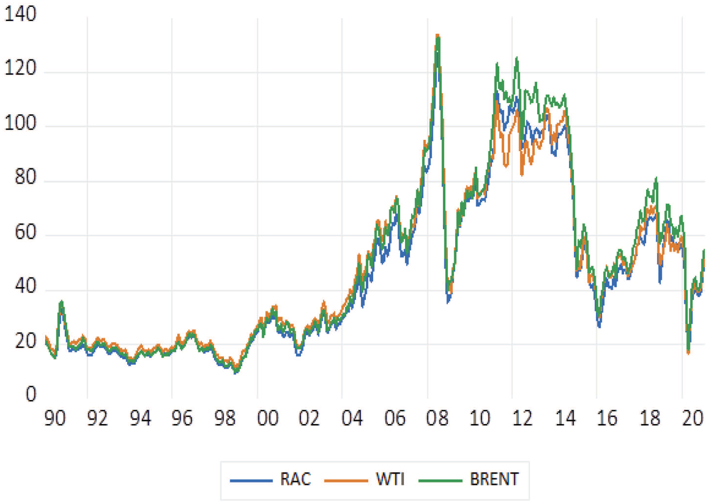
Nominal (spot) oil price

The need for accurate oil price forecasts, given the aforementioned abrupt changes, stems from the fact that they form important decision-making inputs for a number of stakeholders, including private businesses, central banks and the national governments. For instance, Alquist et al. (2013) provide evidence that oil price forecasts help industrial sector companies to forecast their product prices. Moreover, they indicate that investment decisions regarding climate change and carbon emissions predictions, as well as, formulation of regulatory policies in the energy sector may significantly be influenced by oil price forecasts. In addition, Baumeister (2014) shows that oil price forecasting is an important tool for monetary authorities given that it conveys information about predictions in inflation and economic activity. Finally, Baumeister et al. (2018) highlight the importance of oil price forecasts for national governments of both oil-exporters and oil-importers in devising their investment strategies and budget plans. It is also important to highlight that central banks are interested in forecasting real oil prices in domestic currency units, which captures the real cost of oil for domestic consumption (Baumeister and Kilian, 2014). In turn, this further increases the complexity of oil price forecasts as their accuracy further depends of how future exchange rates are estimated.

Moreover, since oil is a physical commodity, it is intuitively expected that its price should be primarily affected by oil market fundamentals, namely unexpected oil supply disruptions, unanticipated changes in global demand for crude oil and unexpected changes in inventory demand (see, for instance, Kilian, 2009; Kilian, 2010; Kilian and Murphy, 2014). However, the more recent literature highlights the significant effect of financial markets as drivers of oil price movements. This is known as the financialisation of the oil market and is primarily related to speculative activity in this market. In this regard, Fratzscher et al. (2014) explain that oil acts as a financial asset due to the fact that it reacts rapidly to information associated with other financial assets such as stock prices or exchange rates. More recently, Degiannakis and Filis (2018) show that apart from the oil market fundamentals, information stemming from the financial markets could improve oil price forecasts.

Based on the aforementioned developments in the oil market, as well as, the complexity of its price forecasts, the literature has developed an array of different forecasting frameworks and has employed a series of different predictors in search of improved accuracy. For instance, early studies that focus on the use of Vector Error Correction models (Coppola, 2008; Murat and Tokat, 2009) or futures-based forecasts (Knetsch, 2007; Alquist and Kilian, 2010) attempt to show whether these forecasts can outperform the random-walk. Other studies, such as those by Baumeister and Kilian (2012), Baumeister and Kilian (2014) and Naser (2016) employ Vector Autoregressive-type (VAR) forecasting frameworks (e.g., structural VARs, time-varying parameter VARs), whereas Baumeister et al. (2014) and Baumeister and Kilian (2014, 2015) assess the predictive accuracy of combined forecasts. Baumeister et al. (2015) and, more recently, Degiannakis and Filis (2018) exploit the advantages of the mixed-data sampling (MIDAS) forecasting framework.

In terms of predictors, the existing studies have more commonly used the oil market fundamentals such as world oil production, global economic activity index, US crude oil inventories among others (see, for example, Baumeister and Kilian, 2012; Baumeister et al., 2015; Rubaszek, 2021). It should be noted also that it is not uncommon for studies to use futures prices (see Coppola, 2008; Alquist and Kilian, 2010; Baumeister et al., 2014; Pak, 2018) and product spreads (see Baumeister et al., 2018) as potential predictors. Furthermore, recent studies, such as those by Baumeister et al. (2015), Degiannakis and Filis (2018) and Zhang and Wang (2019), assess the predictive information of financial data in oil price forecasts. Turning to the data frequency, we note that for most studies data are collected and reported monthly, although quarterly frequencies are also reported (see Baumeister et al., 2014). In addition, the use of financial data allows to assess whether higher frequency data (daily or weekly) could improve the forecasting accuracy of oil prices.

The choice of the crude oil price benchmark is another interesting distinction among the existing studies. There are three main variables, namely, the US refiners’ acquisition cost (RAC), the West Texas Intermediate (WTI) and the Brent crude oil (Brent), which are used extensively in the forecasting exercises. Pertaining to the readily available information, empirical studies that forecast both WTI and RAC include Alquist et al. (2013), Baumeister et al. (2015), Baumeister and Kilian (2015), Wang et al. (2017) and Baumeister et al. (2018). In addition, authors such as Coppola (2008), Alquist and Kilian (2010), Naser (2016) and Rubaszek (2021) focus on the WTI price forecasts, whereas other studies such as Knetsch (2007), and Degiannakis and Filis (2018) concentrate solely on the Brent crude oil prices. Finally, authors who develop forecasting frameworks for both WTI and Brent benchmarks include Chen (2014), Funk (2018), and Zhang and Wang (2019).

We should emphasise that the aim of this study is not to provide a thorough review of the related literature. Rather, with the aforementioned considerations in mind, we perform a meta-analysis approach, which has been proven to be a useful methodical tool for integrating the empirical findings of numerous existing studies. Each oil price forecasting study presents different results given the use of different modelling frameworks, data frequencies, forecast horizons, and sample periods, among others. However, when these empirical results are systematically combined and reviewed, we are able to identify and interpret the various factors that contribute the most to higher forecast accuracy. Therefore, the meta-analysis technique is important in order to provide meaningful interpretations regarding differences in forecasting accuracy from one study to another.

Hence, given the increasing interest in this line of research and the numerous papers that have been published, especially in the last 15 years, our study makes an important contribution by providing a quantitative navigation that will allow to explore those factors that systematically provide more accurate oil price forecasts. In this regard, this is the first meta-analysis attempt in this line of research. For this purpose, we employ a Bayesian Model Averaging (BMA) model, which facilitates the investigation of the factors leading to more accurate forecasts across the different studies.

Our findings can be succinctly summarised as follows. First, MIDAS and combined forecasting frameworks, among other forecasting techniques, exhibit significantly higher forecasting accuracy. Second, the use of Brent crude oil price generates better predictions in comparison with other crude oil benchmarks. Finally, the short-run forecasting horizons and the use of real oil price also contribute to lower forecast errors.

The remaining of the paper is structured as follows. Section 2 describes the data collection process. Section 3 presents the empirical method, while Section 4 discusses the main results along with robustness checks. Finally, Section 5 concludes the study.

2. Forecasts errors across literature

2.1 Data collection

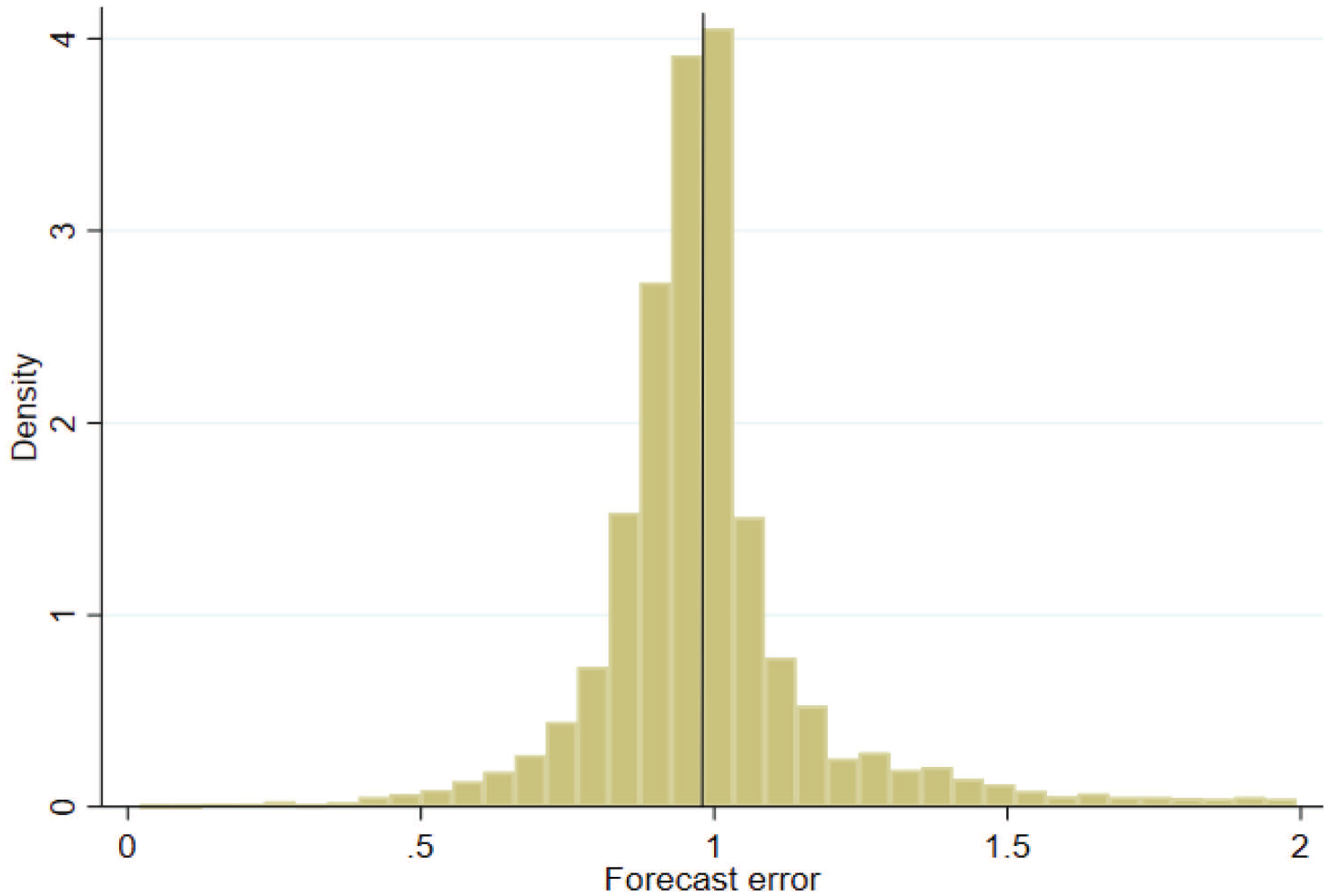
A significant part of the forecasting literature uses the random walk (RW) without a drift, (also known as the no-change forecast), as the benchmark forecasting framework Its h-month ahead forecast error at any time point is shown as $e_{t + h | t}^{R W} = O_{t + h | t} - O_{t + h}$ , where o represents the price of oil. Furthermore, the root mean squared error (RMSE, thereafter) is used as the main loss function to measure the forecasting accuracy. The forecasting accuracy of the RW forecasting framework can be defined as follows:

R M S E_{h}^{R W} = \sqrt{\frac{1}{T} \sum_{t = 1}^{T} {(e_{t + h | t}^{R W})}^{2}},

(1)

where t =1…T denotes the out-of-sample forecasting observations. Furthermore, h shows the h-month ahead forecast horizon that takes values from 1 up to N months ahead. For instance, $R M S E_{1}^{R W}$ is the RMSE of the RW model for the 1-month ahead horizon, $R M S E_{2}^{R W}$ denotes the RMSE for the 2-month ahead horizon, and so on. It is also very common for studies to report the forecasting performance of competing forecasting frameworks in relative terms against the RMSE of the RW forecasting framework. This can be calculated as follows:

R R M S E_{h l}^{m} = ψ_{h l}^{m} = (R M S E_{h l}^{m}) / (R M S E_{h l}^{R W}),

(2)

where the superscript m denotes a forecasting model other than the random walk, while hl indicates the h-month ahead horizon from study l. When the ratios are lower than one then the competing model is able to outperform the benchmark model. The main variable of interest in our study is the relative RMSE (RRMSE, thereafter).¹ We use the terms $R R M S E_{h l}^{m}, ψ_{h l}^{m}$ and ‘relative forecasting performance’ interchangeably throughout the remainder of this paper.

We perform a Google scholar search using the key combinations ‘oil price predictability’, ‘oil price forecasts’, ‘oil price forecasting’ and ‘oil price modelling’. In order to impose a certain quality threshold, we only focus on published papers. The inclusion of working papers, many of which produce large horse-races of forecasts, would make the total amount of observations intractable. This search was carried out between July and September 2021.

The next step is to impose a number of criteria according to which a study can be included in our sample. Our first criterion requires for a study to report at least one RMSE or RRMSE, which is the metric that we focus on. Therefore, the papers that report on alternative evaluation metrics for the relative forecasting performance (such as the direction of change statistic) are excluded.

The second criterion is associated with the great number of combinations of forecasting techniques and the corresponding RMSEs or RRMSEs, and thus, we only collect on the reported RMSEs or RRMSEs that use random walk as the benchmark forecasting framework. ² Therefore, the reported RMSEs or RRMSEs that are based on different benchmark are not included in our meta-sample. Our third criterion is related to the use of non-standard machine learning strategies (such as random forests and artificial neural networks) from a number of papers the last years. As a result, we focus on traditional econometric models and thus we excluded those studies. In this way, we ensure the comparability of the collected RRMSEs across studies.³

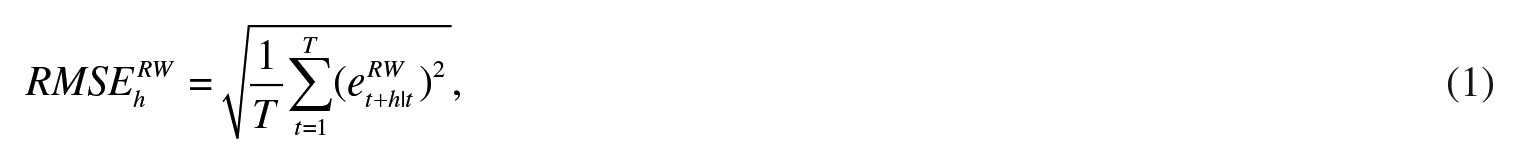
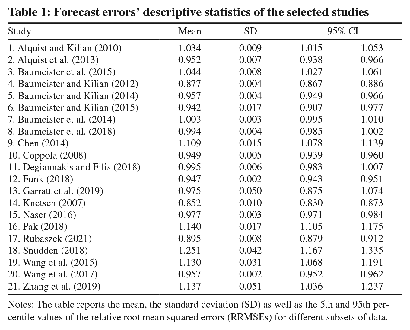
Overall, the total sample consists of 6,089 observations collected from 21 papers. Table 1 presents the summary of the selected studies, together with the descriptive statistics of their RRMSEs. Figure 2 presents the histogram of the selected RRMSEs, which exhibits fat tails, showing a wide range of forecast errors. The selection process is summarised in a PRISMA chart in Appendix 1, while the full list of studies is provided in Appendix 2.

Table 1:

Forecast errors’ descriptive statistics of the selected studies

Study	Mean	SD	95% CI
1. Alquist and Kilian (2010)	1.034	0.009	1.015	1.053
2. Alquist et al. (2013)	0.952	0.007	0.938	0.966
3. Baumeister et al. (2015)	1.044	0.008	1.027	1.061
4. Baumeister and Kilian (2012)	0.877	0.004	0.867	0.886
5. Baumeister and Kilian (2014)	0.957	0.004	0.949	0.966
6. Baumeister and Kilian (2015)	0.942	0.017	0.907	0.977
7. Baumeister et al. (2014)	1.003	0.003	0.995	1.010
8. Baumeister et al. (2018)	0.994	0.004	0.985	1.002
9. Chen (2014)	1.109	0.015	1.078	1.139
10. Coppola (2008)	0.949	0.005	0.939	0.960
11. Degiannakis and Filis (2018)	0.995	0.006	0.983	1.007
12. Funk (2018)	0.947	0.002	0.943	0.951
13. Garratt et al. (2019)	0.975	0.050	0.875	1.074
14. Knetsch (2007)	0.852	0.010	0.830	0.873
15. Naser (2016)	0.977	0.003	0.971	0.984
16. Pak (2018)	1.140	0.017	1.105	1.175
17. Rubaszek (2021)	0.895	0.008	0.879	0.912
18. Snudden (2018)	1.251	0.042	1.167	1.335
19. Wang et al. (2015)	1.130	0.031	1.068	1.191
20. Wang et al. (2017)	0.957	0.002	0.952	0.962
21. Zhang et al. (2019)	1.137	0.051	1.036	1.237

Notes: The table reports the mean, the standard deviation (SD) as well as the 5th and 95th percentile values of the relative root mean squared errors (RRMSEs) for different subsets of data.

Figure 2:

Histogram of RRMSEs

2.2 Heterogeneity of forecasts errors

In order to examine the heterogeneity of the reported RRMSEs across the literature, we look into three categories. From each category we identify factors that may systematically influence the reported RRMSEs. We describe this process in the following paragraphs.

Oil price. Primarily, we focus our attention on the oil price that is forecasted in the published studies. We posit that there could be oil price benchmarks that are harder to predict. If this holds true, forecasters should be aware so as to engage in efforts to improve their forecasting frameworks for these benchmarks. In line with the collected papers, we concentrate on three oil price benchmarks. The first is the West Texas Intermediate (WTI). Therefore, we create a dummy variable that takes 1 when the RRMSE comes from a forecasting exercise that uses WTI and 0 otherwise. Secondly, we consider the US refiners’ acquisition cost (RAC) as an alternative price index. In a similar vein, we use a dummy variable that takes 1 when the RRMSE comes from an analysis that uses RAC and 0 otherwise. Finally, we use the Brent benchmark which serves as our base category. Another feature of the oil price is whether the forecasting exercise uses the nominal or real price. Thus, we create an additional moderator variable (‘real’) that takes 1 for the real and 0 for the nominal oil price.

Forecasting Framework. First, we treat as the base category the relative forecasting performance of the frameworks that belong to the ARIMA family. Mathematically, this can be formalised by:

ψ_{h l}^{A R I M A} = (R M S E_{h l}^{A R I M A}) / (R M S E_{h l}^{R W}) .

(3)

Second, we create the moderator variable ‘structural’ that takes 1 when the RRMSE comes from a structural framework, either a structural VAR or a DSGE. Third, we create the dummy variable ‘midas’ where a value of 1 is assigned when a MIDAS framework is used. In a similar fashion, we use the same type of moderator dummy variables for frameworks using regression-based forecasts (‘regression’), combined forecasts (‘combined’) and finally, frameworks that use futures prices (‘future’) and product spreads (‘product’).⁴

Forecasting Features. Finally, we consider three features of the forecasting exercise. The first characteristic is the forecasting horizon (the variable is named ‘horizon’). The collected studies that constitute our meta-sample use different data frequencies. Therefore, the forecasting horizon is expressed in different frequencies. Following Eickmeier and Ziegler (2008), we convert the horizons into months in order to obtain a homogeneous measure across all studies. The ‘horizon’ takes values from 1 up to h, depending on the h-months ahead horizon of each study l. For robustness, we also follow Chinn and Meese (1995) and we create a dummy variable where one (1) is assigned to the short-run forecast horizons (up to 12-months ahead) and zero (0) to the long-run horizons (more than 12-months ahead).⁵

The second characteristic is the forecasting period. More precisely, we take into account the date of the end-of-sample, as the forecast errors are reported for the end of the sample period. In this way, we examine whether there is a trend in the reported results.

The third characteristic is associated with the use of real-time forecasts which are introduced by Baumeister and Kilian (2012) and followed by other authors in the literature of this particular area of research. We additionally take this characteristic into account by including the variable ‘real-time’ that takes 1 when real-time forecasts are reported.

Table 2 presents a reflection of the three forecasting groups and the variables under consideration, while Figure 3 provides a graphical illustration of the heterogeneity of the reported estimates across the three different categories.

Table 2:

List of Moderator Variables

Variable Name	Description
Forecasting Frameworks
ARIMA	ψ_hl from an ARIMA model (base category)
Structural	1 if ψ_hl from a structural model
MIDAS	1 if ψ_hl from a MIDAS model
Regression	1 if ψ_hl from a regression-based model
Combined	1 if ψ_hl from a combined forecast model
Future	1 if ψ_hl from a futures-based model
Product	1 if ψ_hl from a product spread-based model
Oil Price
Brent	ψ_hl from using Brent (base category)
WTI	1 if ψ_hl uses West Texas Intermediate
RAC	1 if ψ_hl uses US refiners’ acquisition cost
Oil Price
Real	1 if ψ_hl uses real price
Forecasting Features
Horizon	Number of months
Period	Standardized date of the end-of-sample
Real-time	1 if ψ_hl uses real-time forecasts

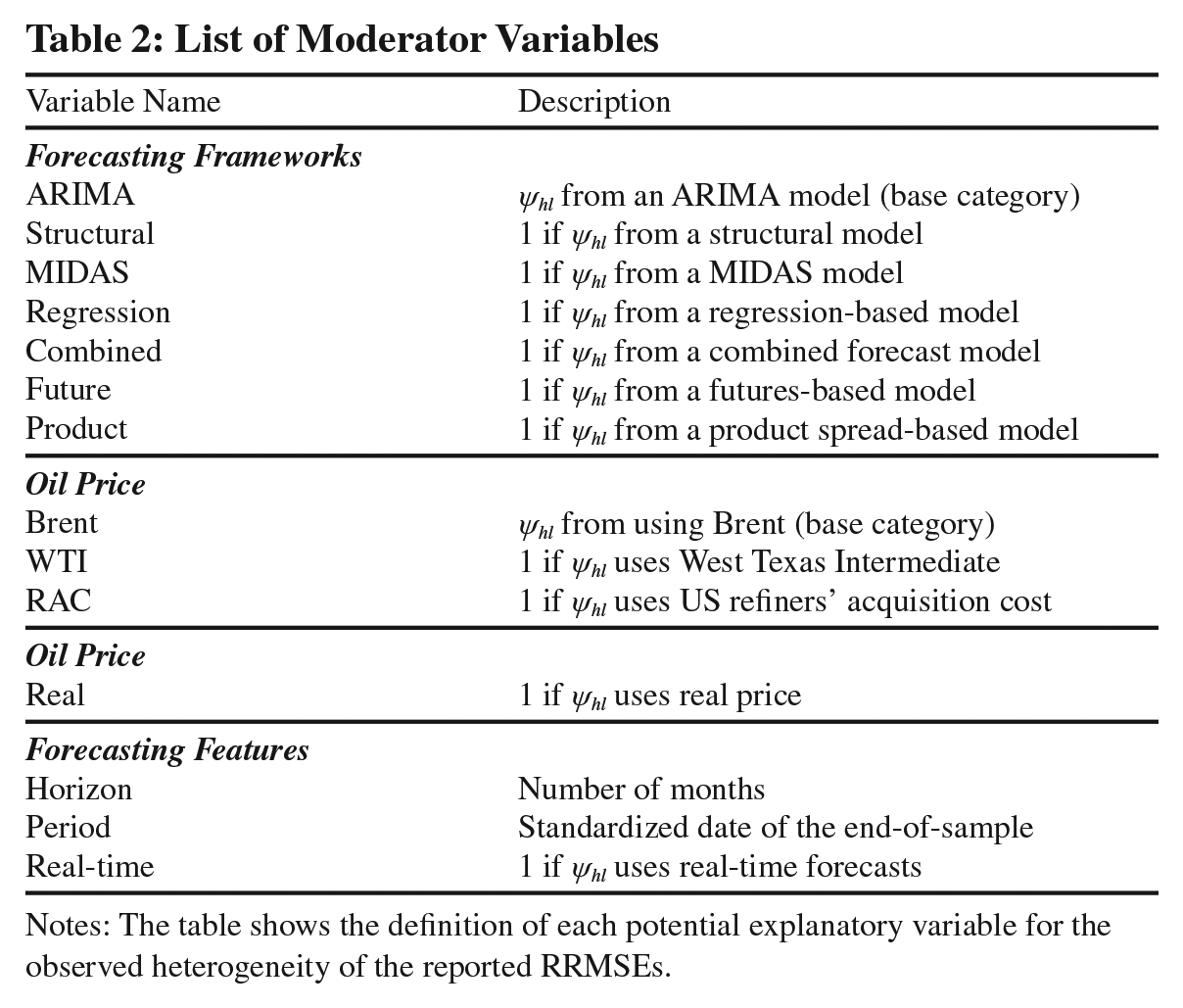
Notes: The table shows the definition of each potential explanatory variable for the observed heterogeneity of the reported RRMSEs.

Figure 3:

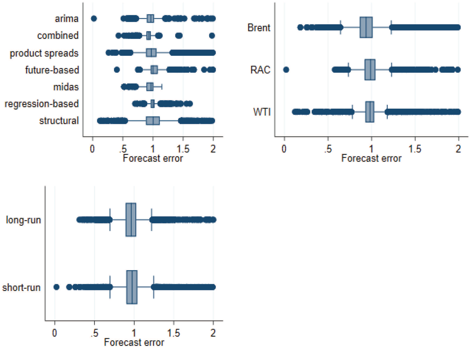
Heterogeneity of RRMSEs across different forecasting frameworks, prices and horizons

3. Methodology

This section presents the method according to which the factors that systematically affect the reported estimates can be identified. The benchmark method is the Bayesian Model Averaging (BMA) that belongs to the family of models that deal with big data (Koop, 2017). The usefulness of this technique is properly revealed when the number of regressors is quite large. Overall, BMA remains an increasingly popular method of identifying the significant drivers of a specific variable (here the RRMSE). Our meta-regression model can be written as:

ψ_{h l} = c + \sum_{S = 1}^{12} γ_{S}^{ξ} Z_{S, h l} + ε_{h l},

(4)

where ψ_hl is the h-month ahead horizon’s relative forecast error from study l, Z depicts the moderator variables described in Section 2.2, γ_s are the coefficients of each moderator and the subscript S is the indicator of each moderator. In total, we have 12 moderator variables, and therefore S ∈ [1,12]. As usual, the error term, ε, is normally distributed; ε ~ N(0,σ). The superscript ξ indicates that the equation (4) is valid under model M_ξ of the BMA exercise. In our case, the use of 12 regressors results in 4,096(=2¹²) different models to choose from. This means that the model space consists of M₁,…,M_ξ models, where ξ ∈ [1,…,4096]. Due to the moderate number of explanatory variables, it is computationally feasible to evaluate and average all model specifications. At the same time, the analytical solution can also be derived. We estimate the posterior model density as well as the posterior inclusion probabilities both analytically and computationally. The results from both approaches are identical.

The main characteristic of the model averaging techniques is that they assign a weight to each model and then, average across these models. Therefore, the inference is not based on individual models, but instead on weighted averages. Even with a small number of regressors, the model space consists of many potential combinations. In the remaining part of this Section, we present the basic concepts of the BMA. Appendix 3 provides a more detailed technical discussion. Based on the Bayes’ rule, the posterior density of γ is written as:

p (γ | ψ, Z) = \sum_{j = 1}^{4096} p (γ_{j} | ψ, Z, M_{j}) p (M_{j} | ψ, Z),

(5)

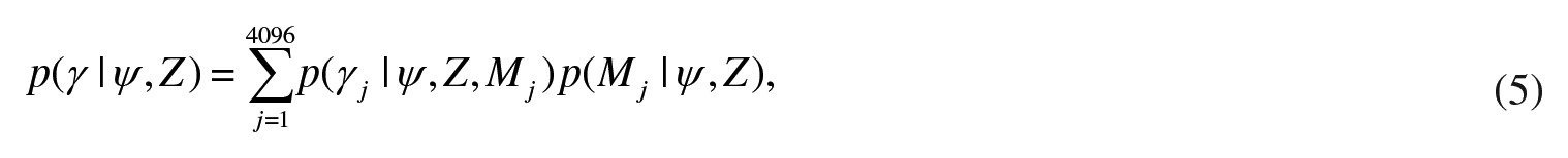
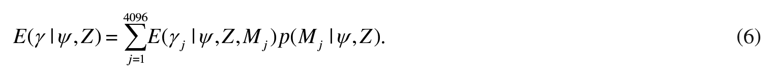
where p(γ_j | ψ, Z, M_j) is the posterior distribution under model M_j and p(M_j |ψ, Z) is the posterior model probability.⁶ The above equation shows that the posterior model probabilities are used as weights. More precisely, the posterior density of γ for each model M_j is weighted by the posterior model probability of each model M_j. The point estimates for the posterior mean can be derived by taking expectations:

E (γ | ψ, Z) = \sum_{j = 1}^{4096} E (γ_{j} | ψ, Z, M_{j}) p (M_{j} | ψ, Z),

(6)

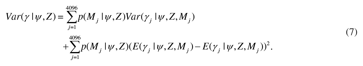
The posterior variance is proved to be:

\begin{array}{l} V a r (γ | ψ, Z) = \sum_{j = 1}^{4096} p (M_{j} | ψ, Z) V a r (γ_{j} | ψ, Z, M_{j}), \\ + \sum_{j = 1}^{4096} p (M_{j} | ψ, Z) {(E (γ_{j} | ψ, Z, M_{j}) - E (γ_{j} | ψ, Z, M_{j}))}^{2}, \end{array}

(7)

To help better understand our benchmark model, it is instructive at this point to consider the posterior inclusion probability (PIP) metric which is defined as the sum of posterior model probabilities of all models that include the specific regressor and takes the following form:

P I P_{i} = \sum_{j = 1} p (M_{j} | ψ, Z),

(8)

with i ∈ [1,12] indicating that each regressor has a specific inclusion probability. Therefore, the PIP shows how frequently a regressor appears in the alternative M_j models. In this way, the level of PIP determines whether a regressor can be considered as a robust determinant. The value of the PIP ranges between zero and one, where a value close to one for a particular regressor denotes larger explanatory power. In other words, the variable with the highest estimated PIP is this variable that is present in almost all alternative model specifications and therefore, a robust driver that explains the heterogeneity of the reported estimates.

As far as the parameters priors are concerned, we choose the following options. As there is no prior knowledge, we use non-informative priors for the intercept and the variance; p(c) ∝1 and p(σ) ∝ σ⁻¹. Regarding the γ parameters, we assume that they are centered at zero and the variance is proportional to $σ^{2} (g {(Z_{i}^{'} Z_{i})}^{- 1})$ , where g is the Zellner’s g hyperparameter that indicates the level of uncertainty (the forecasters’ prior belief that the γ parameters are zero). A small (large) g indicates few (many) prior coefficient variance and therefore the lower (higher) the forecasters’ uncertainty. In summary, the coefficients’ distribution depends on g:

γ_{i} | g \sim N (0, σ^{2} (g {(Z_{i}^{'} Z_{i})}^{- 1})) .

(9)

In this study, we employ two different choices regarding g. Firstly, we set g = N, which is the unit information prior (UIP), where N is the sample size. Secondly, we set the hyper-g prior as suggested by Liang et al. (2008). For the case of model priors, we also use two alternative choices. Firstly, we use the uniform model prior that assumes equal probability to all models. Secondly, we relax this assumption by setting a beta-binomial prior. The approximation of the posterior distribution is simulated by a MCMC sampler algorithm.

4. Results

4.1 Main evidence

Table 3 shows the first round of results. Following Kass and Raftery (1995), we categorise the effect of a variable as weak, positive, strong, and decisive if its PIP lies between 0.5–0.75, 0.75–0.95, 0.95–0.99 and 0.99–1, respectively. We begin our analysis with the evaluation of the relative performance of the different forecasting frameworks. The results suggest that the MIDAS frameworks, as well as, the combined forecasts tend to generate significantly lower forecast errors. Such forecasting frameworks have the ability to outperform the ARIMA framework, given the negative and significant coefficients. By contrast, the use of structural-based, regression-based, futures-based, as well as, forecasts based on product spreads, does not seem to significantly outperform the forecasting accuracy of the ARIMA framework.

Table 3:

Bayesian Model Averaging results

	BMA₁			BMA₂
Variable	PIP	post Mean	post SD	PIP	post Mean	post SD
Forecasting Frameworks
Structural	0.048	0.001	0.004	0.104	0.002	0.007
MIDAS	0.981^b	−0.057	0.016	0.977^b	−0.057	0.016
Regression	0.029	−0.001	0.003	0.055	−0.001	0.004
Combined	0.999^a	−0.083	0.009	0.999^a	−0.082	0.010
Future	0.086	0.003	0.013	0.123	0.005	0.014
Product	0.039	0.001	0.004	0.091	0.002	0.006
Oil Price
WTI	0.999^a	0.049	0.009	0.999^a	0.049	0.009
RAC	0.999^a	0.058	0.010	0.999^a	0.058	0.010
Real	0.951^b	−0.072	0.023	0.954^b	−0.072	0.023
Forecasting Features
Horizon	0.999^a	0.003	0.000	0.999^a	0.003	0.000
Period	0.001	0.006	0.001	0.001	0.006	0.001
Real-time	0.084	0.001	0.004	0.143	0.002	0.006

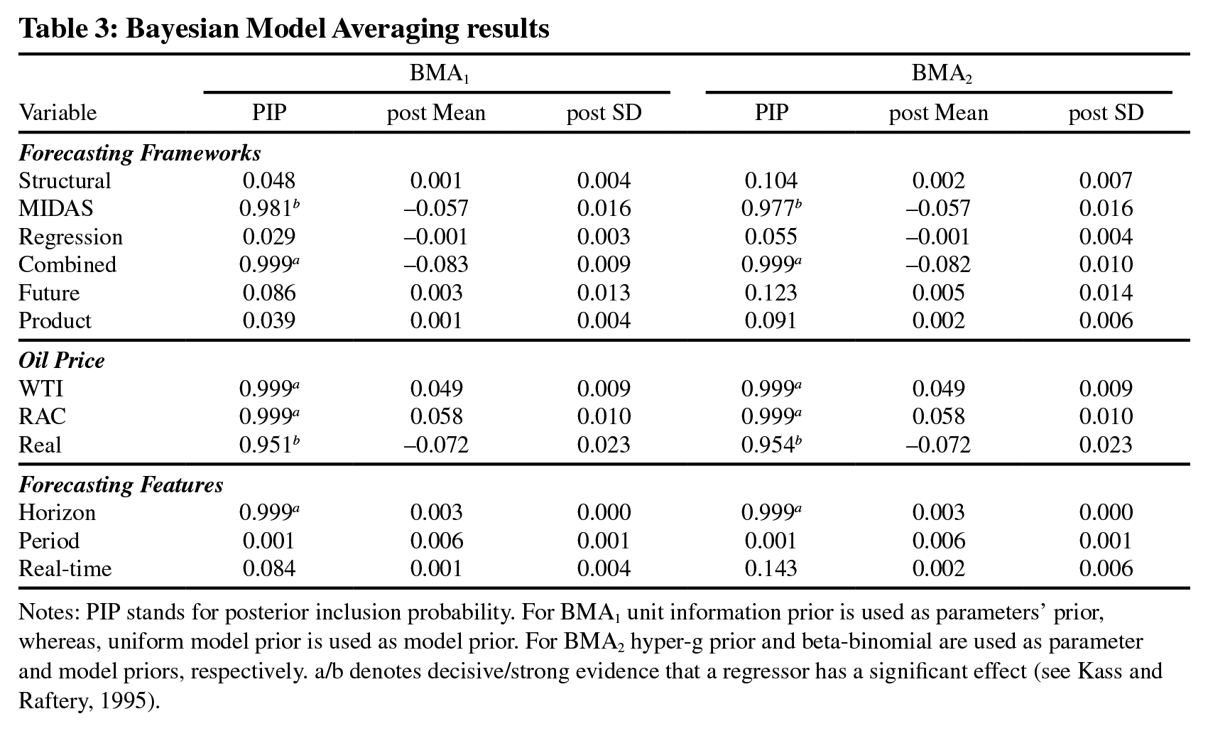
Notes: PIP stands for posterior inclusion probability. For BMA₁ unit information prior is used as parameters’ prior, whereas, uniform model prior is used as model prior. For BMA₂ hyper-g prior and beta-binomial are used as parameter and model priors, respectively. a/b denotes decisive/strong evidence that a regressor has a significant effect (see Kass and Raftery, 1995).

The fact that MIDAS models tend to produce lower forecast errors can be interpreted as follows. The related literature has shown that oil price forecasts are impacted by the fundamental factors of the oil market (i.e., unanticipated changes in oil supply, oil demand, and inventory levels). However, recent research efforts (Degiannakis and Filis, 2018) have also shown that the oil market has become more financialised, meaning that it has become more interconnected with other global financial markets (such as the stock markets, or foreign exchange, among others). Considering that these asset markets convey information to the oil market at a much higher frequency, relatively to the oil market fundamentals, our finding suggests that the use of such higher-frequency financial data, tends to improve oil price forecasts at lower frequencies. This is a feature only available to the MIDAS framework.

With reference to the improved predictive accuracy of combined forecasts frameworks, we maintain that such forecast combinations act as insurance against the poorer forecasting performance of the individual frameworks. Hence, when combining forecasts the weak performance of an individual forecasting framework can be counterbalanced by the better performance of another framework, leading to an overall improvement in the forecast accuracy. This argument is also evident in the work of Baumeister and Kilian (2015) who employ forecast (pooled) combinations. Furthermore, different forecasting strategies exhibit superior forecasting performance at different horizons. Consequently, their combination improves the overall forecasting performance. Therefore, we note that information derived from combined forecasts helps to provide significant predictive gains.

Turning our attention to the choice of the oil price benchmark, our results suggest that the forecasting exercises that use either the US refiners’ acquisition cost (RAC) or the WTI crude oil price tend to report higher RRMSEs compared to those studies that use the Brent crude oil price, given the positive and significant coefficients. Alquist et al. (2013) argue that although the RAC can be used to approximate global oil price movements, it cannot be viewed as the indicative proxy for the price that US refineries paid for crude oil. In this regard, Baumeister et al. (2014) are supportive in favour of the WTI spot price. According to them, the WTI is not subject to revisions and it is also available without delays, which is not the case when the RAC is considered. This could justify the higher forecast error of the RAC compared to the Brent price.

Furthermore, the WTI is considered to be more volatile than the Brent, which makes it harder to be accurately predicted. Possible reasons can be found in the geographical area that they are produced and the transportation costs. Brent is extracted at sea and transferred by ships, which makes it to be less dependent on abrupt changes in transportation costs. By contrast, the WTI is drilled in landlocked regions and thus, its price is affected by both higher transportation costs as well as pipeline bottlenecks and higher storage constraints (Baumeister and Kilian, 2015). Overall, our arguments help to clarify the reasons why the use of Brent appears to provide better forecasting performance. Such findings are also in accordance with Manescu and Van Robays (2014) and Degiannakis and Filis (2018) who propose the importance to use the Brent spot price.

Even more, the WTI crude oil market has attracted the attention of the non-commercial investors, via its futures contracts. Indeed, the WTI has the most liquid and actively traded futures contracts in the crude oil market compared with Brent (Buyuksahin et al., 2013). This explains why the WTI is regarded as a valuable financial asset by energy traders. Such trading activity results in higher volatility for the WTI, which could further explain the lower forecasting accuracy for this crude oil benchmark. Such finding has important implications for end-users of oil price forecasts. Let us assume that there is a Permian Basin operator who is interested in forecasting the price of oil to help guide current production decisions. It is apparent that the appropriate oil price measure to forecast is the price of WTI. In this case, the operator should be aware that her forecasting framework should be improved so as to accommodate the fact that the WTI is harder to predict.

As far as the difference between real and nominal oil prices is concerned, our evidence shows a negative and significant coefficient, which indicates lower forecast errors for the real oil price. This suggests that forecasts of the real price tend to be better than forecasts of the nominal one. A plausible explanation for this finding can be traced at the effect of inflation. More specifically, the higher forecast errors of the nominal oil prices could be explained by the fact that they have an inflation component, which adds uncertainty to the future path of oil prices. Put differently, nominal oil price forecasts make also implicit assumptions about the future inflation, hence they are harder to predict.

Interestingly enough, we do not find evidence that the real-time forecasts are superior. Real-time forecasts are based on datasets that take into consideration delays in reporting relevant information or potential revisions in data series (for instance, this is particular relevant for oil production information). According to Alquist et al. (2013) and Baumeister et al. (2014), forecasters who ignore such constraints in the data series, tend to produce better forecasts. Nevertheless, our findings do not lend support to this claim.

Furthermore, ‘horizon’ appears to have a positive and significant coefficient. This means that longer forecasting horizons produce higher RRMSEs, indicating a lower forecast performance.⁷ This is a plausible finding given that at longer horizons we expect the autoregressive and moving-average components of oil prices to prevail relatively to the fundamentals of the oil market or the financial information. By contrast, we do not find any significant influence on the quality of forecasts from the forecasting period moderator, suggesting that either the more recent or the earlier forecasts in our dataset do not seem to exhibit different levels of predictive accuracy. Such finding could potentially suggest that the oil market maintains a certain level of unpredictability even under the use of the more recently developed forecasting frameworks and data availability (e.g., MIDAS framework and intra-day data). This could be explained by the fact that since 2003 there is a regime change in the behaviour of oil prices, as already mentioned in Section 1. More specifically, prices have become more volatile, adding extra difficulty to the forecaster to generate significantly improved forecasts in the more recent years, relatively to the earlier period. Therefore, it is not entirely unexpected that this variable is not found statistically significant.

4.2 Robustness tests

Having analysed the first round results, it is important to use an array of robustness tests so as to verify the stability of our findings. The first test is to replace the Bayesian setting (BMA) with a frequentist one (FMA) which allows us to maintain the basic rational of model averaging techniques. In this respect, the main difference between frequentist and Bayesian averaging is the construction of weights. Instead of using posterior model probabilities, the new weights are replaced with information criteria. In our exercise, we follow the approach proposed by Magnus et al. (2010) and extended by Amini and Parmeter (2012) who select the weights by minimising the Mallows criterion (Hansen, 2007). The main benefit is that this version of FMA is based on the orthogonalisation of the covariate space that leads to the significant reduction of the models that need to be estimated. In our case, the model space is not an issue due to the moderate number of regressors, as explained in the previous Sections.

The second test is to apply a pure frequentist least squares exercise without using any weighting scheme. Table 4 shows the results for both FMA and OLS with clustered standard errors at study level. Applying both types of frequentist analysis leads to results that are quantitatively and qualitatively similar to the BMA.

Table 4:

Frequentist Model Averaging and Least Squares

	FMA		OLS
Variable	Coefficient	SD	Coefficient	SD
Forecasting Frameworks
Structural	−0.039	0.041	0.027	0.056
MIDAS	−0.039*	0.032	−0.042	0.045
Regression	−0.019	0.029	0.002	0.046
Combined	−0.033*	0.024	−0.067**	0.033
Future	0.000	0.021	0.033	0.042
Product	0.001	0.018	0.026	0.041
Oil Price
WTI	0.035*	0.022	0.049*	0.018
RAC	0.047*	0.037	0.057**	0.027
Real	−0.075*	0.044	−0.065	0.044
Forecasting Features
Horizon	0.004*	0.000	0.003***	0.001
Period	0.000	0.001	0.006	0.004
Real-time	0.070	0.114	0.011	0.018

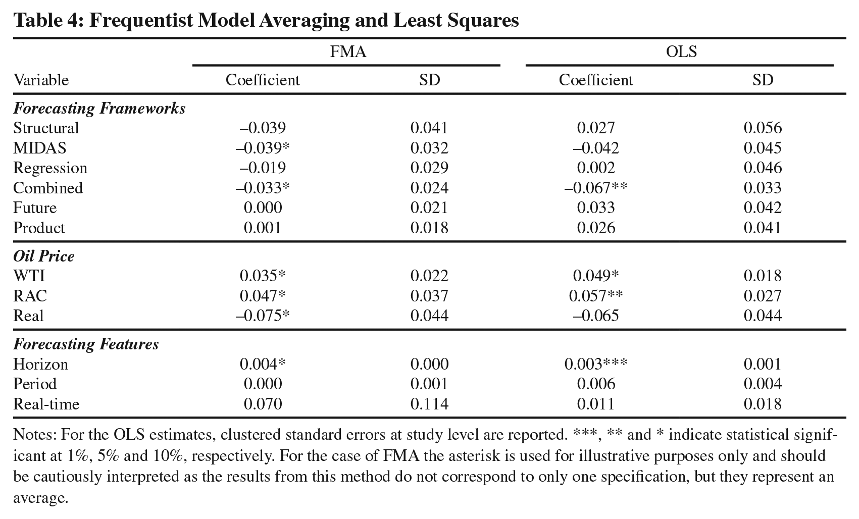
Notes: For the OLS estimates, clustered standard errors at study level are reported. ***, ** and * indicate statistical significant at 1%, 5% and 10%, respectively. For the case of FMA the asterisk is used for illustrative purposes only and should be cautiously interpreted as the results from this method do not correspond to only one specification, but they represent an average.

Overall, the moderator variables that were found to be robust drivers of the observed heterogeneity of the forecast errors remain the same; MIDAS and combined forecasts frameworks tend to have a better performance. The opposite is true when the forecasting exercises are based on the WTI and RAC oil price benchmarks. The horizon does continue to play a role, with longer horizons resulting in worse forecasts. Finally, when the focus is on real prices, then these forecasts are superior compared to those based on nominal prices.

Finally, we apply a variant of the least absolute shrinkage and selection operator (LASSO). This method combines the concept of minimising the least squares along with a shrinkage process that removes the drivers that are not important. The minimisation process can be written as: ${(ψ_{h l}^{m} - \sum_{S = 1}^{12} γ_{s} Z_{S, h l})}^{2} + λ \sum_{S = 1}^{12} | γ |$ , where λ is the shrinkage parameter. Even though the number of regressors is not very large, the insertion of a shrinkage parameter provides a natural way to test the robustness of model averaging. To this point, we adopt its more widely used Bayesian version. Under certain assumptions regarding the prior distributions, the outcome is a set of estimations for those γ coefficients that have not being shrunk to zero.⁸ Therefore, the variables that still have a non-zero coefficient after the shrinkage process are the most robust drivers that explain the forecasting ability. The results are shown in Table 5. As in the frequentist exercise, MIDAS and combined forecasts frameworks continue to report lower forecasts errors. In a similar vein, the use of Brent price tends along with using real prices to provide better forecasts across the examined literature. Once more, better forecasts come from shorter forecasting horizons.

Table 5:

LASSO estimates

Variable	post Mean	post SD	post τ
Forecasting Frameworks
Structural	0.000	0.000	0.000
MIDAS	−0.032	0.002	0.304
Regression	0.000	0.000	0.000
Combined	−0.092	0.004	0.401
Future	0.000	0.001	0.004
Product	0.000	0.000	0.000
Oil Price
WTI	0.034	0.004	0.185
RAC	0.022	0.003	0.155
Real	0.029	0.004	0.158
Forecasting Features
Horizon	0.015	0.004	0.011
Period	0.000	0.000	0.000
Real-time	0.001	0.001	0.001

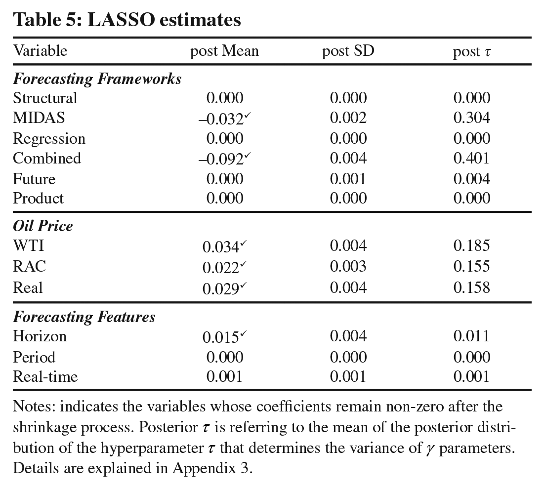
Notes: indicates the variables whose coefficients remain non-zero after the shrinkage process. Posterior τ is referring to the mean of the posterior distribution of the hyperparameter τ that determines the variance of γ parameters. Details are explained in Appendix 3.

5. Conclusions

The aim of this paper is to provide a comprehensive assessment of the factors that contribute to improve oil price forecasts, by conducting a meta-analysis. The period of time of the paper stems from the fact that since the early 2000’s and the regime change in oil price fluctuations, there is an ever-increasing interest in oil price forecasts. However, despite the numerous efforts, there is no empirical evidence to summarise the different findings from different studies and identify the key factors that contribute to the accuracy of such forecasts. Thus, our quantitative survey on forecasting characteristics contributes to the practice of oil price forecasting. To the best of our knowledge, this is the first study that attempts to detect the factors that play an important role in oil price prediction by focusing on the relative root mean squared error (RRMSE) metric. We employ a Bayesian Model Averaging (BMA) method which is used to combine information from various forecasting characteristics in order to produce an accurate predictive performance.

Using a dataset that covers a large range of different forecasting frameworks, datasets, horizons and oil price benchmarks, we attempt to identify the most importance drivers of the forecasting accuracy. Based on the RRMSE metric, we summarise our findings as follows. First, the choice of the forecasting framework plays an important role. MIDAS and combined forecasts provide systematically better predictions than other forecasting strategies. Second, the price benchmark is also an important factor. Our evidence indicates that the forecasting ability is improved when the Brent price is used, whereas the opposite holds when the WTI or the RAC are employed. Finally, shorter forecasting horizons, as well as the use of real prices generate forecasts of greater accuracy. By contrast, the forecasting period and the real-time datasets are not important factors of the forecasting ability. Our findings remain unchanged under a set of different robustness tests.

The results of the present study have important implications for various stakeholders. Forecasting characteristics contain information that help financial market participants (traders and energy investors), policy makers, multinational corporations, and the oil industry, among other stakeholders, to improve oil price forecasts. Considering financial market participants, accurate oil price forecasts convey information regarding future oil price returns. Given that oil is also regarded as a financial asset, energy investors and traders should pay attention to superior forecasts in order to make better decisions regarding allocation of funds or portfolio risk estimation, among others. Similarly, policy makers benefit from accurate oil price forecasts in order to develop macroeconomic policies that help to prevent economic recessions, tackle inflationary pressures or boost industrial production. Furthermore, accurate oil price forecasts offer important information to the oil industry companies in terms of their financing, investment and managerial decisions related to their capital expenditure, market share, earnings expectations and stock price performance, among others. Additionally, multinational corporations are significantly benefited by accurate oil price forecasts and thus corporate decision making managers could be able to create strategies to mitigate the impact of higher oil price for example, in order to reduce the effect of rising costs on production.

For the purposes of the current meta-analysis, we make use of the RRMSE which is the most frequently used metric of forecasting performance. Therefore, a potential venue for future research in this field of study could be the consideration of alternative forecasting accuracy metrics, such as the directional accuracy. The extent to which alternative measures behave differently within the context of this type of empirical analysis may trigger attempts for more accurate oil price forecasts and thus such attempts are expected to intensify in the future.

Supplemental Material

sj-pdf-1-enj-10.5547_01956574.45.2.mfil – Supplemental material for Evaluating Oil Price Forecasts: A Meta-analysis

Supplemental material, sj-pdf-1-enj-10.5547_01956574.45.2.mfil for Evaluating Oil Price Forecasts: A Meta-analysis by Michail Filippidis, George Filis and Georgios Magkonis in The Energy Journal

Footnotes

Appendices

Acknowledgements

We would like to thank the handling editor (Prof. David C. Broadstock) and three anonymous referees for their constructive comments on a previous version of the paper. In addition, we would also like to thank the participants of the 2022 International Symposium on Environmental and Energy Finance Issues (ISEFI) Conference and the 2022 International Research Meeting in Business and Management (IRMBAM), for their helpful suggestions. The usual disclaimer applies.

1.

See .

2.

argue that the conventional random walk forecast is uninformative in terms of forecast accuracy and should not be used for forecasting comparisons of aggregated data. However, our decision to employ the random walk based on the fact that this benchmark is widely used in the literature on forecasting oil prices.

3.

For simplicity, we use the term RRMSE to the remainder of the paper.

4.

See for a brief discussion of these methods.

5.

The VIF statistics do not support the existence of multicollinearity. The values are available upon request.

6.

To avoid unnecessary confusion, we will use ψ instead of $ψ_{h l}^{m}$ for the remaining of the paper.

7.

This result remains the same when we use a dummy variable for measuring the horizon assigning 1 for shorter forecasts (up to 12 months) and 0 otherwise.

8.

See for technical details.

References

Alquist

Kilian

. (2010) “What do we learn from the price of crude oil futures?” Journal of Applied Econometrics 25(4): 53973. https://doi.org/10.1002/jae.1159.

Alquist

Kilian

Vigfusson

R.J.

(2013) “Forecasting the price of oil.” In Handbook of Economic Forecasting Vol. 2, Part A 42707. https://doi.org/10.1016/B978-0-444-53683-9.00008-6.

Amini

S.M.

Parmeter

C.F.

(2010) “Comparison of model averaging techniques: Assessing growth determinants.” Journal of Applied Econometrics 27(5): 87076. https://doi.org/10.1002/jae.2288.

Baumeister

(2014) “The art and science of forecasting the real price of oil.” Bank of Canada Review Spring, 21-31.

Baumeister

Guérin

Kilian

(2015) “Do high-frequency financial data help forecast oil prices? The MIDAS touch at work.” International Journal of Forecasting 31(2): 23852. https://doi.org/10.1016/j.ijforecast.2014.06.005.

Baumeister

Kilian

(2012) “Real-time forecasts of the real price of oil.” Journal of Business & Economic Statistics 30(2): 32636. https://doi.org/10.1080/07350015.2011.648859.

Baumeister

Kilian

(2014) “What central bankers need to know about forecasting oil prices.” International Economic Review 55(3): 86989. https://doi.org/10.1111/iere.12074.

Baumeister

Kilian

(2015) “Forecasting the real price of oil in a changing world: a forecast combination approach.” Journal of Business & Economic Statistics 33(3): 33851. https://doi.org/10.1080/07350015.2014.949342.

Baumeister

Kilian

Lee

T.K

. (2014) “Are there gains from pooling real-time oil price forecasts?” Energy Economics 46: S33-S43. https://doi.org/10.1016/j.eneco.2014.08.008.

10.

Baumeister

Kilian

Zhou

(2018) “Are product spreads useful for forecasting oil prices? An empirical evaluation of the Verleger hypothesis.” Macroeconomic Dynamics 22(3): 56280. https://doi.org/10.1017/S1365100516000237.

11.

Benmoussa

A.A.

Ellwanger

Snudden

(2020) “The new benchmark for forecasts of the real price of crude oil.” No. 20209. Bank of Canada Staff Working Paper.

12.

Bernanke

B.S.

(2005) “Remarks by Governor Ben S. Bernanke at the Sandridge lecture, Virginia association of economics, Richmond, Virginia.”.

13.

Buyuksahin

Lee

T.K.

Moser

J.T.

Robe

A.M.

(2013) “Physical markets, paper markets and the WTI-Brent spread.” The Energy Journal 34(3): 12953. https://doi.org/10.5547/01956574.34.3.7.

14.

Chen

S.-S.

(2014) “Forecasting crude oil price movements with oil-sensitive stocks.” Economic Inquiry 52(2): 83044. https://doi.org/10.1111/ecin.12053.

15.

Chinn

M.D.

Meese

R.A.

(1995) “Banking on currency forecasts: how predictable is change in money?” Journal of International Economics 38(1): 16178. https://doi.org/10.1016/0022-1996(94)01334-O.

16.

Coppola

(2008) “Forecasting oil price movements: Exploiting the information in the futures market.” Journal of Futures Markets 28(1): 346. https://doi.org/10.1002/fut.20277.

17.

Degiannakis

Filis

(2018) “Forecasting oil prices: High-frequency financial data are indeed useful.” Energy Economics 76: 38802. https://doi.org/10.1016/j.eneco.2018.10.026.

18.

ECB (2015) “Forecasting the price of oil.” ECB (2015) ECB Economic Bulletin 4: 878.

19.

Eickmeier

Ziegler

(2008) “How successful are dynamic factor models at forecasting output and inflation? A meta-analytic approach.” Journal of Forecasting 27(3): 23765. https://doi.org/10.1002/for.1056.

20.

Fratzscher

Schneider

Van Robays

. (2014) “Oil prices, exchange rates and asset prices.” ECB working paper No. 1689. https://doi.org/10.2139/ssrn.2442276.

21.

Funk

Christoph

(2018) “Forecasting the real price of oil-Time-variation and forecast combination.” Energy Economics 76: 28802. https://doi.org/10.1016/j.eneco.2018.04.016

22.

Hansen

B.E.

(2007) “Least squares model averaging.” Econometrica 75(4): 1175189. https://doi.org/10.1111/j.14680262.2007.00785.x.

23.

Kass

R.E.

Raftery

A.E.

(1995) “Bayes factors.” Journal of the American Statistical Association 90(430): 77395. https://doi.org/10.1080/01621459.1995.10476572.

24.

Kilian

, (2009) “Not all oil price shocks are alike: Disentangling demand and supply shocks in the crude oil market.” American Economic Review 99(3): 1053069. https://doi.org/10.1257/aer.99.3.1053.

25.

Kilian

(2010) “Oil price volatility: Origins and effects.” WTO Staff Working Paper No. ERSD-2010-02.

26.

Kilian

Murphy

D.P.

(2014) “The role of inventories and speculative trading in the global market for crude oil.” Journal of Applied Econometrics 29(3): 45478. https://doi.org/10.1002/jae.2322.

27.

Knetsch

T.A.

(2007) “Forecasting the price of crude oil via convenience yield predictions.” Journal of Forecasting 26(7): 52749. https://doi.org/10.1002/for.1040.

28.

Koop

(2017) “Bayesian methods for empirical macroeconomics with big data.” Review of Economic Analysis 9(1): 336. https://doi.org/10.15353/rea.v9i1.1434.

29.

Liang

Paulo

Molina

Clyde

M.A.

Berger

J.O.

(2008) “Mixtures of g priors for Bayesian variable selection.” Journal of the American Statistical Association 103(481): 41023. https://doi.org/10.1198/016214507000001337.

30.

Magnus

J.R.

Powell

Prüfer

(2010) “A comparison of two model averaging techniques with an application to growth empirics.” Journal of Econometrics 154(2): 13953. https://doi.org/10.1016/j.jeconom.2009.07.004.

31.

Manescu

Van Robays

(2014) “Forecasting the Brent oil price addressing time-variation in forecast performance.” ECB Working Paper 1735. https://doi.org/10.2139/ssrn.2493129.

32.

Murat

Tokat

(2009) “Forecasting oil price movements with crack spread futures.” Energy Economics 31(1): 850. https://doi.org/10.1016/j.eneco.2008.07.008.

33.

Naser

(2016) “Estimating and forecasting the real prices of crude oil: A data rich model using a dynamic model averaging (DMA) approach.” Energy Economics 56: 757. https://doi.org/10.1016/j.eneco.2016.02.017.

34.

Pak

(2018) “Predicting crude oil prices: Replication of the empirical results in “What do we learn from the price of crude oil?” Journal of Applied Econometrics 33(1): 16063. https://doi.org/10.1002/jae.2584.

35.

Rubaszek

(2021) “Forecasting crude oil prices with DSGE models.” International Journal of Forecasting 37: 53146. https://doi.org/10.1016/j.ijforecast.2020.07.004.

36.

Wang

Liu

(2017) “Forecasting the real prices of crude oil using forecast combinations over time-varying parameter models.” Energy Economics 66: 33748. https://doi.org/10.1016/j.eneco.2017.07.007.

37.

Zellner

(1986) “On assessing prior distributions and Bayesian regression analysis with g-prior distributions.” In Bayesian Inference and Decision Techniques in Honor of Bruno de Finetti ( Goel

P.K.

Zellner

, eds.), North-Holland, Amsterdam, 23343.

38.

Zhang

Y.-J.

Wang

J. L.

(2019) “Do high-frequency stock market data help forecast crude oil prices? Evidence from the MIDAS models.” Energy Economics 78: 19201. https://doi.org/10.1016/j.eneco.2018.11.015.

Supplementary Material

Please find the following supplemental material available below.

For Open Access articles published under a Creative Commons License, all supplemental material carries the same license as the article it is associated with.

For non-Open Access articles published, all supplemental material carries a non-exclusive license, and permission requests for re-use of supplemental material or any part of supplemental material shall be sent directly to the copyright owner as specified in the copyright notice associated with the article.

0.00 MB

0.03 MB