Offshore Market Design in Integrated Energy systems: A Case Study on the North Sea Region towards 2050

Abstract

Offshore grids, with multiple interacting transmission and generation units connecting to the shores of several countries, are expected to have an important role in the cost-effective energy transition. Such massive new infrastructure expanding into a new physical space will require new offshore energy market designs. Decisions on these designs today will influence the overall value potential of offshore grids in the future. This paper investigates different possible market configurations and their impacts on operational costs and required congestion management, as well as prices and emissions. We use advanced integrated energy system optimisation, applied to a study case on the North Sea region towards 2050. Our analysis confirms the well-known concept of nodal pricing as the most preferable market configuration. Nodal pricing minimises costs (0.2–1.6 b€/year lower) and CO₂ emissions (0.6–5.6 Mton/year lower) with respect to alternative market designs investigated. The performance of the different market designs is highly influenced by the overall architecture of the offshore grid, and the rest of the energy system. E.g., flexibility options help reducing the spread between the designs. But the results are robust: nodal pricing in offshore grids emerges as the preferable market configuration for a cost-effective energy transition to carbon neutrality.

Keywords

Offshore grids Market design Congestion management Integrated energy systems Optimisation

1. Introduction

1.1 Background

To achieve climate goals and to mitigate the consequences of climate change, energy systems need to reduce emissions to sustainable levels (IPCC, 2022). To decarbonise the energy systems, variable renewable energy (VRE) generation, as well as adequate market design (Newbery, 2018), are likely to be of high value. Solar photovoltaic (PV) and wind energy are becoming more and more competitive with respect to technologies burning fossil fuels (IRENA, 2019). Particularly in Europe, offshore wind generation in the North Sea is likely to play a significant role in achieving the climate goals, and that is why the European Commission is promoting its development (The European Commission, 2020b).

Previous studies have found that it is cost-effective to develop some of the offshore wind development in advanced offshore grid configurations (Gea-Bermúdez et al., 2020; Konstantelos et al., 2017; Koivisto et al., 2019; Gea-Bermúdez et al., 2022) owing to savings in capital expenditure due to economies of scale and increased flexibility of the transmission lines that are part of offshore grids. On the other hand, the potential value that offshore grids can bring to the energy system has been found to be highly dependent on the level of sector coupling between the electricity, heat, and transport sector (Gea-Bermúdez et al., 2022). Offshore grids can both be used to generate and transport electricity, but also to generate other fuels, like hydrogen (H₂). As an example, Denmark is considering generating green H₂ on the energy island they are planning to develop (DW, 2021).

Considering the vast potential of offshore wind in the North Sea, it is important to investigate the influence that offshore grids can have on the energy markets (not only the electricity one), and how different market designs influence such impact. The market design of offshore grids can play a significant role in the overall value of offshore grids, since it can influence, among other things, investment incentives and congestion management costs. Inspired by the North Sea Wind Power Hub project (North Sea Power Hub, 2020), Tosatto et al. (2021) investigated the influence of an energy island on the European power system by 2030 showing how exporting countries are affected by the lower electricity prices. A similar study has been performed by Jansen et al. (2022). Both Jansen et al. (2022) and Tosatto et al. (2021) assumed nodal pricing in their papers, which according to Commission et al. (2020) would be the one ideal in Europe, since it perfectly reflects all costs of supplying electricity at given nodes and, manages congestion at the same time. However, nodal pricing is not free from problems, since its implementation might cause some market flaws.

The main shortcoming of nodal pricing is—according to one strain of the literature—missing market liquidity and the possibility for suppliers to exercise market power in the grid nodes, which have a few or a single electricity generator. Although some studies find evidence that combining nodes to a large market zone might even exacerbate market power and increase the profits of the dominant company (see Harvey and Hogan, 2000), another part of the literature argues for reduced market power when going from nodal to zonal pricing or potentially increased market power when separating a market zone into more and smaller ones (e.g., Frank A.Wolak, Chairman, 1999; Henney, 1998). Hence, a higher liquidity and, therefore, a more competitive outcome can be achieved by combining several grid nodes in one market zone and thus increasing the number of market players on the generation side and also on the demand side within the zone. With such a configuration, each bidding zone is assumed to contain no significant intra-zonal grid constraints, while the borders between the different zones constitute structural grid constraints. However, if the ignored intra-zonal grid constraints are large, it can potentially lead to high congestion management (Bertsch et al., 2017), the so-called redispatch, and high related costs (Holmberg and Lazarczyk, 2015). The magnitude of this influence in offshore grids is something that has not been investigated yet. Given the fact that offshore grids in the North Sea will mostly connect producers rather than consumption (apart from some offshore H₂ generators who will act as consumers of offshore electricity on site) and that there will be several wind parks connected to one offshore grid node, it is likely that the possibility of exercising market power will be reduced. However, we acknowledge that this is the case under the assumption that all offshore generation is constrained off at the same price. As mentioned above, the nodal as well as zonal designs may still enable the exercise of market power in case of dominant players remain in this configuration. This empirical question needs to be tested, depending on the control of wind generation within constrained regions of the offshore zones.

However, given the fact that nodal pricing theoretically serves as the most efficient benchmark for an electricity market configuration, it is worth investigating and comparing nodal versus several zonal approaches to gain insights into the benefits and costs of different market configurations in the immensely growing offshore electricity sector.

1.2 Contribution to the literature of this paper

The main goal of this study is to investigate and quantify the influence of different offshore electricity market designs on the operation of day-ahead markets in integrated energy systems towards 2050, as well as their impact on the required congestion management. The influence of the overall development of the offshore grids on these previous aspects is also analysed, which can be of high value considering the uncertain development of offshore grids. We use as study case the North Sea region. The model includes energy demands for the electricity, heat and transport sectors. We do this through an advanced optimisation process using the open-source energy system model Balmorel. The main contributions of this paper are listed below.

To our knowledge, this paper is the first one analyzing the influence of different offshore market designs on the operation of day-ahead markets towards 2050.

To our knowledge, this paper is the first one analyzing the influence of different day-ahead electricity market offshore grid designs on the required congestion management of the system towards 2050.

To our knowledge, this paper is the first one analyzing the influence of different offshore grid development on the two previous points.

The model used is an integrated energy system, including demand for electricity, heat, and transport sector. This means that the investigated impact quantifies the impact on the entire energy system and not just the electricity one.

The quantification of the difference for scenarios that seek decarbonisation towards 2050 in integrated energy system will inform policy makers and regulators in important decisions about future system architecture. Implementing nodal markets might be more challenging than implementing a zonal one, so there are likely to be practical trade-offs. As a consequence, obtaining insight into comparative differences between different offshore electricity market designs can be of high value.

The structure of the remainder of the paper is as it follows: Section 2 includes the methodology, data and a description of the scenarios and optimisation approach used. Section 3 presents the results, and provides a critical reflection of them. Finally, Section 4 presents the overall conclusions.

2. Methodology

The energy model Balmorel is used for the analysis based on the combination of the model versions employed in Gea-Bermúdez et al. (2023) and Gea-Bermúdez et al. (2022). The Balmorel model has been extended for this paper to be able to simulate congestion management operation. The Balmorel model and data used are open source (Balmorel community, 2021b,a)¹ In the following, we give an overview of the main elements of Balmorel and focus then on scenario development, which includes the optimisation approach used to derive the scenarios.

Table 1:

Investment cost assumptions and corresponding sources for offshore hubs and selected VRE technologies in M2016/MW (M2016/MWh for storage) per year and technology type. Other relevant assumptions like fixed/variable costs or lifetime are not shown but can be found in (Balmorel community, 2021b).

Technology	2025	2035	2045	Source
Solar PV (AC side)	0.42	0.30	0.26	(Danish Energy Agency, 2021)
Onshore wind	1.27	1.15	1.05	(Danish Energy Agency, 2021)
Offshore wind radial (nearshore, AC, western Denmark)	1.66	1.58	1.51	(Koivisto et al., 2019), (Danish Energy Agency, 2021) (EA Energy Analysis, 2020), (EDMOnet-Bathymetry, 2021)
Offshore wind radial (far offshore, AC, western Denmark)	2.07	1.88	1.74	(Koivisto et al., 2019), (Danish Energy Agency, 2021) (EA Energy Analysis, 2020), (EDMOnet-Bathymetry, 2021)
Offshore wind radial (far offshore, DC, western Denmark)	2.72	2.48	2.31	(Koivisto et al., 2019), (Danish Energy Agency, 2021) (EA Energy Analysis, 2020), (EDMOnet-Bathymetry, 2021)
Hub-connected offshore wind (20 m depth, very close to hub)	2.06	1.84	1.72	(Koivisto et al., 2019), (Danish Energy Agency, 2021) (EA Energy Analysis, 2020), (EDMOnet-Bathymetry, 2021)
Hub-connected offshore wind (20 m depth, close to hub)	2.09	1.87	1.75	(Koivisto et al., 2019), (Danish Energy Agency, 2021) (EA Energy Analysis, 2020), (EDMOnet-Bathymetry, 2021)
Hub-connected offshore wind (20 m depth, far from hub)	2.12	1.90	1.78	(Koivisto et al., 2019), (Danish Energy Agency, 2021) (EA Energy Analysis, 2020), (EDMOnet-Bathymetry, 2021)
Hub-connected offshore wind (30 m depth, very close to hub)	2.17	1.94	1.81	(Koivisto et al., 2019), (Danish Energy Agency, 2021) (EA Energy Analysis, 2020), (EDMOnet-Bathymetry, 2021)
Hub-connected offshore wind (30 m depth, close to from hub)	2.20	1.97	1.84	(Koivisto et al., 2019), (Danish Energy Agency, 2021) (EA Energy Analysis, 2020), (EDMOnet-Bathymetry, 2021)
Hub-connected offshore wind (30 m depth, far from hub)	2.23	2.00	1.87	(Koivisto et al., 2019), (Danish Energy Agency, 2021) (EA Energy Analysis, 2020), (EDMOnet-Bathymetry, 2021)
Offshore hub (platform and equipment)	0.19	0.19	0.17	(Koivisto et al., 2019)

2.1 Balmorel

2.1.1 Generic model description

The energy system model Balmorel (Wiese et al., 2018) is open source (Balmorel community, 2021a), has a flexible structure, is deterministic, and has a bottom-up approach. Over the past years, the model has been developed considerably with the goal of including more energy sectors (Gea-Bermúdez et al., 2021), more detailed electrofuels and H₂ modelling (Bramstoft et al., 2020; Lester et al., 2020; Jensen et al., 2020), and to have a more advanced system operation modelling (Gea-Bermúdez et al., 2021).

Several configurations of the Balmorel model have been applied in this paper to be able to perform capacity development optimisations, day-ahead optimisations, and congestion management optimisations. The possibility to perform congestion management optimisations is a new feature of the model that has been developed to write this paper.

The temporal resolution in Balmorel is composed of years, and each year contains seasons, which contain terms. The simulated years correspond to 2025, 2035, and 2045, which are meant to represent an average of the time periods 2020–2030, 2030–2040, and 2040–2050, respectively. The meaning of seasons and terms is flexible in Balmorel and it is defined by the user. For example, seasons can be used to represent days, weeks, months, etc., while terms can be used to represent hours, minutes, seconds, etc.

The geographical scope applied in this paper covers 10 countries: United Kingdom, Sweden, Belgium, Denmark, France, Netherlands, Finland, Norway, Germany and Poland. Countries are split into regions in the model based on existing bidding zones. The exception is Germany, that is split into four bidding zones in the model to capture existing intra-country bottlenecks. In total we model 37 biding zones (21 onshore + 16 offshore hubs). Within the same bidding zone, transmission constraints are ignored, while between different zones the transmission is limited mainly by the interconnector capacities.

While considering different market zones, we have considered the inter-zonal bottlenecks and existing market configurations in most countries. At the same time, by splitting Germany into four model regions, we believe in having captured the intra-zonal network bottlenecks in one of the countries with the largest and growing congestion management needs (Kunz, 2013; Bundesnetzagentur, 2021). The growing congestion stems from the fact that Germany is still organized as one market zone in electricity trading. However, since we model Germany in four zones, our model probably captures a large share of the congestion issues that a model with more zones would capture. This can be seen as a proxy and modelling simplification for the flow-based market coupling that takes place in reality, mainly in the Central-Western European (CWE) market area.

The energy system modelling includes energy demands of the electricity, heat, and transport sectors. The energy demands of these sectors are modelled as electricity, heat, and H₂ demand (Figure 1). European or national decarbonisation goals towards 2050 of the transport sector are applied in the paper. Figure 2 illustrates the potential synergies that are captured in the model.

Figure 1:

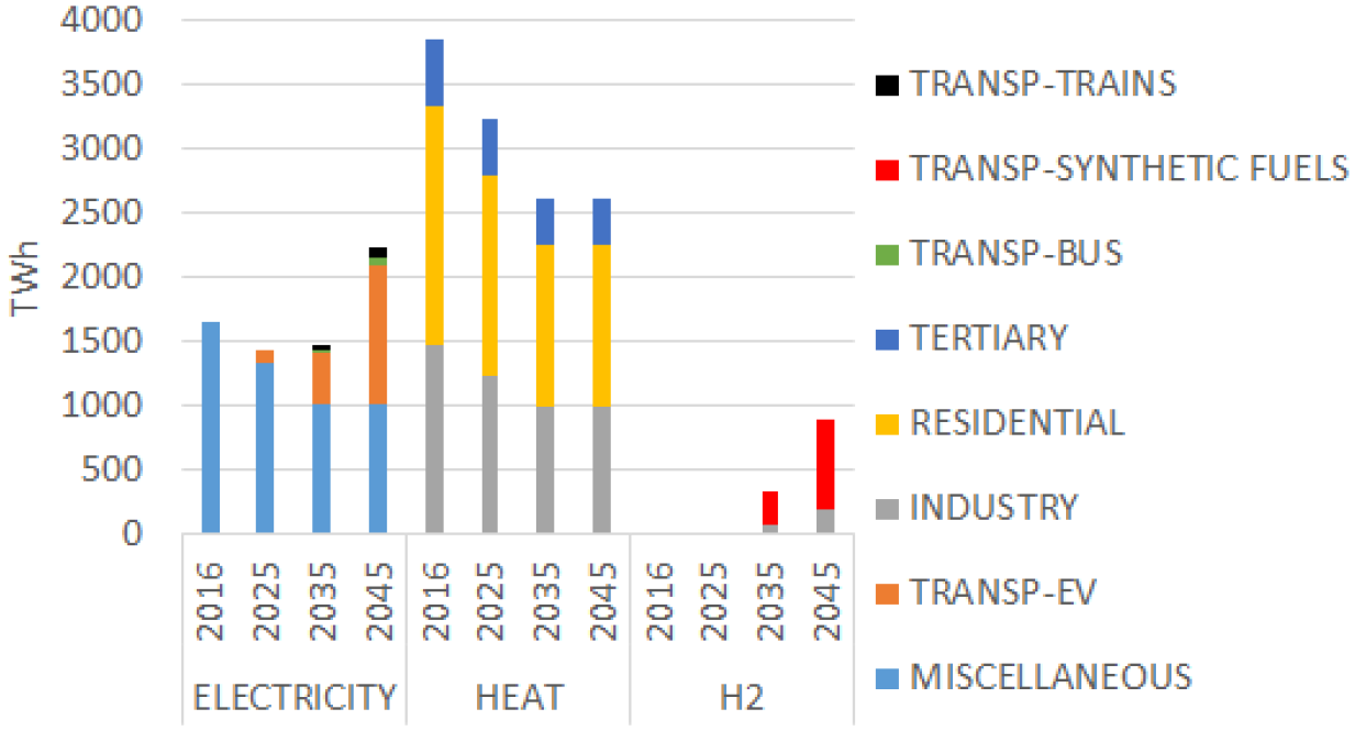
Total exogenous demand assumed in the studied countries per commodity, year, and sector (TWh). The year 2016 is considered as the base year of the model and is not included in the optimisations. H₂ stands for hydrogen. Figure obtained from GeaBermúdez et al. (2022).

Figure 2:

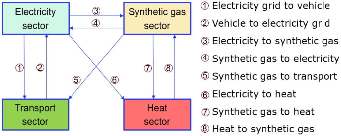
Possible synergies between all the sectors included in the model. Figure obtained from Gea-Bermúdez (2021).

The generic objective of the optimisation model is to minimise discounted system costs (Equation 1) while satisfying the energy needs of the consumers. In the absence of market power (as it is assumed in this paper), modelling market clearing as an optimisation problem is equivalent to modelling it as an equilibrium problem since they share the same Karush–Kuhn–Tucker conditions. Part of the annual demand for the different commodities is assumed to be exogenous (Figure 1), although additional demand can take place due to sector coupling and/or storage/transmission losses. The different costs of each of the years (y) studied are grouped in fixed costs $(c_{y}^{f o m})$ , variable costs $(c_{y}^{v o m})$ , and investment expenses $(c_{y}^{i n v})$ of the different generation, storage, and transmission infrastructure technologies included in the model (listed in Section 2.1.2). Fixed costs and investment expenses are only relevant for the optimisation of long-term capacity planning. All costs in the model are annualised in the objective function, whereas an interest rate of 4% is used to discount and annualise investment-related costs (Danish Energy Agency, 2021). The interest rate used assumes a social planner perspective. Investments are annualised to make a fair comparison of the different technologies, due to the possibility of them having different lifetimes. Variable costs include fuel costs, operation costs, and CO₂ taxes.

The overall decision variables in the model are investment capacities in different technologies (generation/storage units, H₂ pipelines, electricity transmission, district heating expansion), and technology operation per term (energy generation, storage content, storage loading, energy trade, and electric vehicle (EV) operation). The storage content of hydro reservoirs without pumping is modelled per season though, meaning that the energy content per term is not modelled. Another variable which is optimised in the model is generation and storage unit mothballing. Mothballing means that units can be not available for operation during one year, to avoid paying the annual fixed costs, and then become operative again in future years. At the end of their technical lifetime, the units are forced to be decommissioned. Decommissioning costs of exogenous units are not part of the model.

Future years are discounted to reflect the socio-economic value of time using an annual discount rate of 4% (Danish Energy Agency, 2021), which is used to calculate the resulting discount factor (DF_y) of each modelled year. If only one year is optimised at a time, then the discounting is not relevant.

\min_{c_{y}^{f o m}, c_{y}^{v o m}, c_{y}^{i n v}} \sum_{y} D F_{y} \cdot (c_{y}^{f o m} + c_{y}^{v o m} + c_{y}^{i n v})

(1)

Other key equations in the model are commodity balances (electricity balance, heat balance, etc.), technology-specific operational constraints, storage balance, and resource potentials, e.g., maximum installed onshore wind capacity.

Additional special equations, variables, and costs, e.g., unit commitment-related ones (on/ off status, ramping limits, minimum up-time, etc.), are also part of the model. However, they are by default not activated, unless the user finds it relevant. The complexity of the model can increase significantly when activating these special parts of the model.

2.1.2 Modelling energy system components

Generation and storage technologies: Numerous generation and storage technologies are part of the optimisation and compete with each other. The technologies included are dispatchable generation units (hydro reservoirs, electric power-to-heat units (electric heaters, electric boilers, and heat pumps), fuel boilers, combined heat and power (CHP), non-CHP thermal units, fuel cells, electrolysers, and methanation-direct air capture. Other technologies included are non-dispatchable generation units (wind onshore, wind offshore, solar PV, solar heating) and storage units (H₂ steel tanks, electric batteries, hydro pumping, heat water tanks, pit thermal storage). Technology data is mostly based on Danish Energy Agency (2021). Overall the data assumes a considerable reduction of wind and solar PV costs towards 2050 (Table 9). More cost information can be accessed in Gea-Bermúdez et al. (2023) and Gea-Bermúdez et al. (2022).

Electricity network: Electricity trade between regions is modelled in Balmorel using a net transfer capacity approach based on Gunkel et al. (2020). Transmission losses per km distinguish between alternate current (AC) and direct current (DC) lines. Distribution losses for generation and storage technologies are included. Such losses depend on how far from the main high voltage grid the technologies are assumed to be. Investment expenses for electricity transmission lines are derived by using the distance between the centroids of the modelled regions. Such costs and corresponding losses are based on Nordic Energy Research and International Energy Agency (2016) and Gea-Bermúdez et al. (2020). Existing and planned interconnectors are taken from Gea-Bermúdez et al. (2021). The lines are assumed to have a technical lifetime of 40 years (Danish Energy Agency, 2021). Power line protection costs and compensation costs for citizens are not included in the investment cost of the transmission lines. More detailed information can be found in Gea-Bermúdez et al. (2021).

Heat sector: The heat sector includes the energy needs of individual users (in this paper residential and tertiary sectors), industry, and district heating. The modelling of district heating is made considering different network scales based on Münster et al. (2012). District heating expansion is assumed to have a cost of 0.4 M€₂₀₁₆/MW_th (Henning and Palzer, 2014) and a lifetime of 40 years (Danish Energy Agency, 2021). Individual users’ modelling considers the end purpose of heat demand (space heating and hot water). Heat modelling in the industry sector is based on Danish Energy Agency (2021), Rehfeldt et al. (2018), and Wiese and Baldini (2018), and differentiates between three different temperature needs in the heat demand of the industry sector: low temperature (lower than 100°C), medium temperature (100–500°C), and high temperature (higher than 500°C). Technological limits on the output temperature of heat generation units is considered. For instance, heat pumps are only allowed to provide low-temperature heat demand. More information on this sector can be found at Gea-Bermúdez et al. (2021).

Synthetic gas: The synthetic gas sector includes the energy balance in each time step (term) of these two commodities: synthetic natural gas (SNG) and H₂. The modelling is the same as the one used in Gea-Bermúdez et al. (2023).

SNG can be generated through methanation-direct air capture units, which consume heat, H₂ and electricity. SNG can be used as a perfect replacement of natural gas and its CO₂ emissions are not penalised in the objective function as it is assumed to be carbon neutral. The costs, losses and constraints of natural gas networks, in which SNG is assumed to flow, are not included in the model. This means that SNG generated in each of the regions of the model can be freely distributed around the modelled regions.

The H₂ balance is defined for each region in the model. The modelling includes generation of H₂ with alkaline water electrolysis units, transport of H₂ between regions with H₂ pipelines that assume linear bi-directional flow, and network losses. The data related to the transport of H₂ is based on Danish Energy Agency (2021). Inflexible H₂ demand from industry is included and based on European Commission (2018). H₂ demand of the transport sector is modelled as relatively flexible and is explained later in this section. More details can also be found in Gea-Bermúdez et al. (2023).

Transport sector: Decarbonisation of the transport sector is assumed towards 2050 and its demand is split into flexible and inflexible EVs, and demand for synthetic fuels. The capital costs and the operational costs not related to energy consumption of all the different transportation means included in the model (cars, shipping, aviation, etc.) are not considered. The modelling is taken from Gea-Bermúdez et al. (2022).

Inflexible EV annual demand include the electrification of rail transport and buses that are not currently electrified. This annual demand data is taken from Transport and Environment (2018) and is broken down using exogenous time series in each region, with the demand pattern assumed constant for trains, and time dependent for buses. The time dependent patterns for buses is based on Philip Swisher (2020).

Road transport (excluding buses) is modelled as flexible EVs, which are represented as a virtual storage for each model region based on the work of Gunkel et al. (2020). The modelling includes limits to charging and discharging related to usage patterns, the electricity consumed for charging, and a representation of the battery storage in the EV fleet. The main equation of EVs is the hourly virtual storage balance. The balance is defined assuming seasonal cycles, i.e. the level of the storage at the start of each modelled season must equal the level at the end of that season. The model optimizes discharging and charging as well as the virtual storage content of the aggregated EV fleet. The number of EVs towards 2050, which is used as input to derive the time series of EVs, is based on (Philip Swisher, 2020). EVs are divided into battery EVs and plug-in hybrid EVs. Plug-in hybrid EVs are not allowed to be used for vehicle-to-grid purposes, and therefore, can only provide smart charging. Bottom-up modelling of driving patterns is used to generate the time-dependent input parameters used in the model. Vehicle trips are assumed to start when vehicles leave from home and to finish when they return, disregarding the performed activity. It is assumed that most EVs are not connected to the grid during most working hours. Trip consumption is calculated using the distance travelled by vehicles and average drive-train efficiencies. Therefore, different driving behaviours are disregarded. Inflexible charging restricts minimum charging, whereas the charger capacity restricts maximum charging. Furthermore, upper and lower limits for the state of charge are time-dependent and are based on assumptions related to when EVs are at charging stations (see Figure 3). EV charging is penalised with a charging loss and distribution grid losses. Operational and capital costs of EVs are not included. In short, in the model, flexible EVs can provide flexibility via smart charging (since only part of their demand is assumed to be inflexible) and by providing vehicle-to-grid services.

Figure 3:

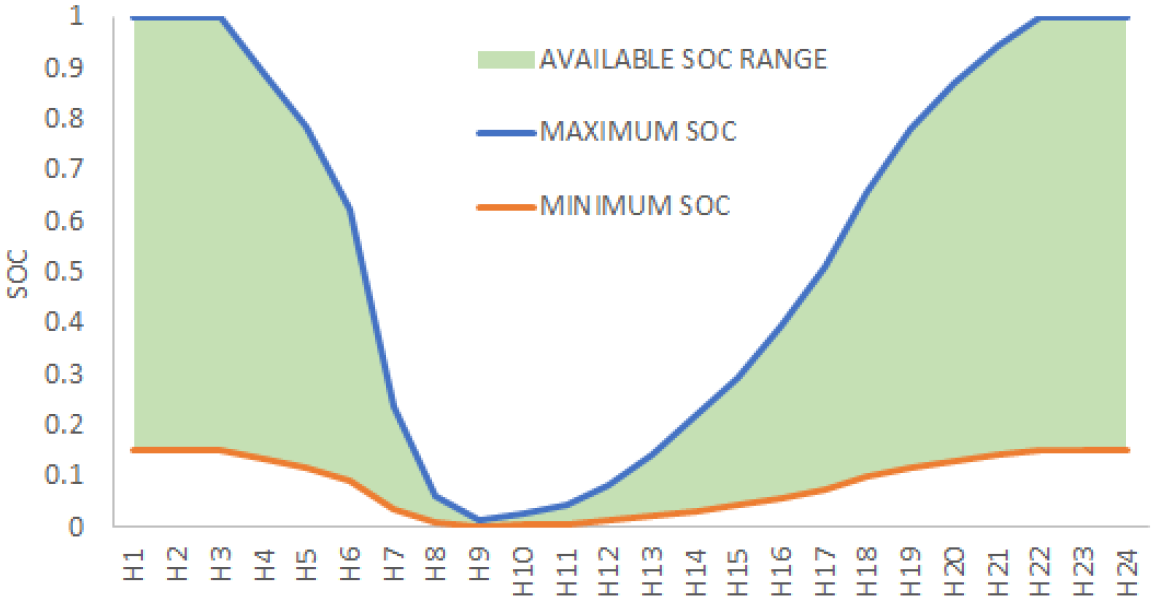
Illustration of the available state of charge (SOC) range during the day of electric vehicles. Figure obtained from Gea-Bermúdez et al. (2022).

The annual synthetic fuel demand required to decarbonise the shipping and aviation transport sectors of the studied countries is included in the scenarios and is based on Transport and Environment (2018). Such demand is modelled as an increasing annual H₂ demand towards 2050 that needs to be satisfied in each onshore region along the year. H₂ can be generated anywhere, but it needs to be sent ultimately to the onshore regions to be consumed. The hourly distribution of this H₂ demand is optimized, although the peak-to-average ratio of such distribution is limited with an upper bound of 1.5 in each region to consider limited flexibility of the technologies that consume such H₂. More information regarding the modelling of this H₂ demand can be found in Gea-Bermúdez et al. (2022).

Investments in biomass units are not allowed in the optimisations, since the generation of synthetic fuels for the transport sector is likely to use a large share of the available biomass resources (Sims et al., 2010). The costs and challenges related to the transport of the biomass resources are not included.

Energy efficiency: The energy efficiency target of 32.5% reduction of final energy consumption by 2030 that the European Commission has established (The European Commission, 2020a) is considered in the model. The exogenous electricity demand assumptions (excluding the transport sector which already includes efficiency measures) and heat demand development towards 2050 consider that such efficiency target takes place. While the European Commission uses the year 2007 as a reference for this target, in this paper the year 2016 is used to make this calculation because of limitations on the availability of data.

Fuel price and CO₂ tax: Fuel prices and CO₂ tax development data towards 2050 is taken from Nordic Energy Research and International Energy Agency (2016). The CO₂ tax helps reducing emissions towards 2050. The CO₂ tax is assumed to be 29.8, 90.4, 120.6€₂₀₁₆/ton in 2025, 2035, and 2045, respectively. No other tax is included. Biofuel data is assumed to be carbon neutral and it is based on Flex4RES project (2019).

Wind and solar modelling: The modelling of wind and solar PV generation technologies is based on Gea-Bermúdez et al. (2020). The solar and wind resources are not uniform inside each of the studied regions. The different resource grades in each of the regions have different investable potential, costs, and time series. Radially-connected offshore wind power plants (OWPP) are divided into three resource grades: near shore and far offshore connected with AC, and far offshore connected with DC. Hub-connected OWPP are explained in detail later. OWPP costs consider the influence of water depth on foundation costs of offshore wind turbines using data from EDMOnet-Bathymetry (2021) and EA Energy Analysis (2020). The CorRES model is used to simulate wind and solar PV time series (Nuño et al., 2018; Koivisto et al., 2019).

The national onshore wind potential for the scenarios (419 GW in total for the investigated countries) is taken from Nordic Energy Research and International Energy Agency (2016). This limit is relatively low, and tries to model low onshore wind social acceptance. Potentials for radially-connected OWPP are based on Koivisto et al. (2019) and Nordic Energy Research and International Energy Agency (2016), whereas large-scale solar PV national potentials are taken from Ruiz et al. (2019). More information regarding the VRE modelling can be found in Gea-Bermúdez et al. (2021).

Offshore grid modelling: The modelling and data of offshore power grids used in the paper combines the work of Gea-Bermúdez et al. (2023) and Gea-Bermúdez et al. (2022).

Introducing the possibility to build an offshore grid allows for multiple configurations of offshore infrastructure. The offshore grid technologies considered for investments in this paper are hub-to-hub and hub-to-shore electricity/H₂ transmission lines/pipes, hub platforms, and hub-connected offshore wind farms, electrolysers, fuel cells, and steel tank H₂ storage. A total of 16 locations in the North Sea to deploy offshore grid technologies are included in the model.

Offshore regions, which are modelled by default as individual regions (bidding zones), can then be used to generate and transport electricity and/or H₂. Along this paper, offshore regions are also interchangeably called hubs. Modelling offshore grids as individual bidding zones allows to capture possible congestion issues of the pipes and electrical interconnectors connected to the hubs. In some of the runs made in this paper, the market configuration of offshore grids is modified (see Section 2.2).

The size of the offshore hub platform located in a particular offshore region is defined with its nameplate electrical capacity $(c a p a c i t y_{y, r}^{p l a t f o r m})$ using Equation 2. The equation makes sure that, for each year (y), hour (h), and region (r), the total capacity of the hub platform in an offshore region is equal to or larger than the sum of the electricity flows $(f l o w_{y, h, r, r^{'}})$ from the offshore region r to other regions (r′) and the demand of electricity of the different electrolysers $(d e m a n d_{y, h, r}^{e l e c t r o l y s e r s})$ located in the offshore region. More details about the modelling of the hubs can be found in Gea-Bermúdez et al. (2022).

c a p a c i t y_{y, r}^{p l a t f o r m} \geq d e m a n d_{y, h, r}^{e l e c t r o l y s e r s} + {\sum f l o w}_{y, h, r, r^{'}} \forall y, \forall h, \forall r

(2)

Wake losses and transmission losses are modelled linked to the size of hub-connected wind farms. The larger the installed capacity of hub-connected wind farms are, the larger the resulting wake losses and transmission losses will be. Detailed information about the modelling of these losses can be found in Gea-Bermúdez et al. (2023).

2.2 Scenarios and optimisation approach

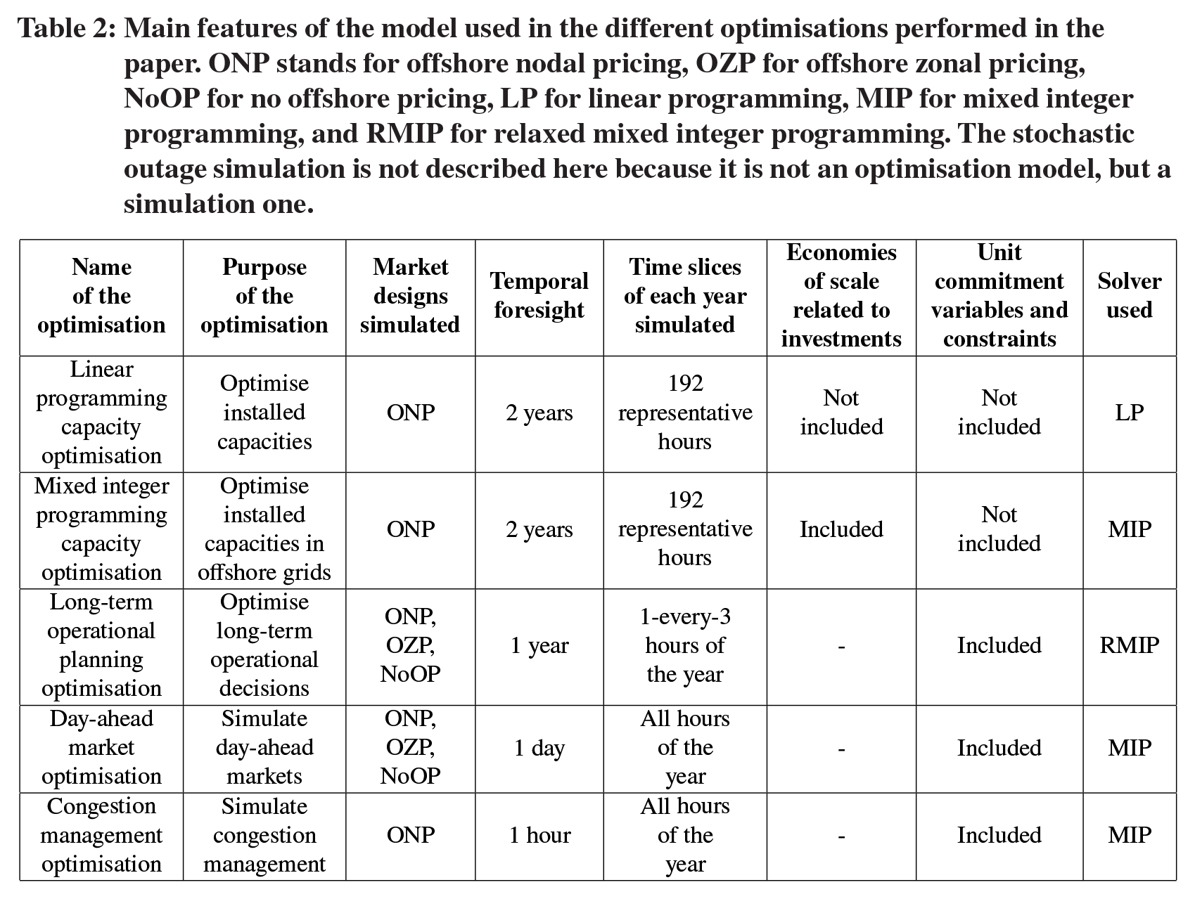
The purpose of this paper is to investigate the impact that different offshore electricity market designs have on integrated energy systems towards 2050, as well as their influence on the required congestion management of the system. To achieve this objective a sequence of optimisations and simulations, illustrated in Figure 4, are performed. Each optimization applies a different configuration of the Balmorel model. The main features of the model used in the different optimisations are presented in Table 2.

Figure 4:

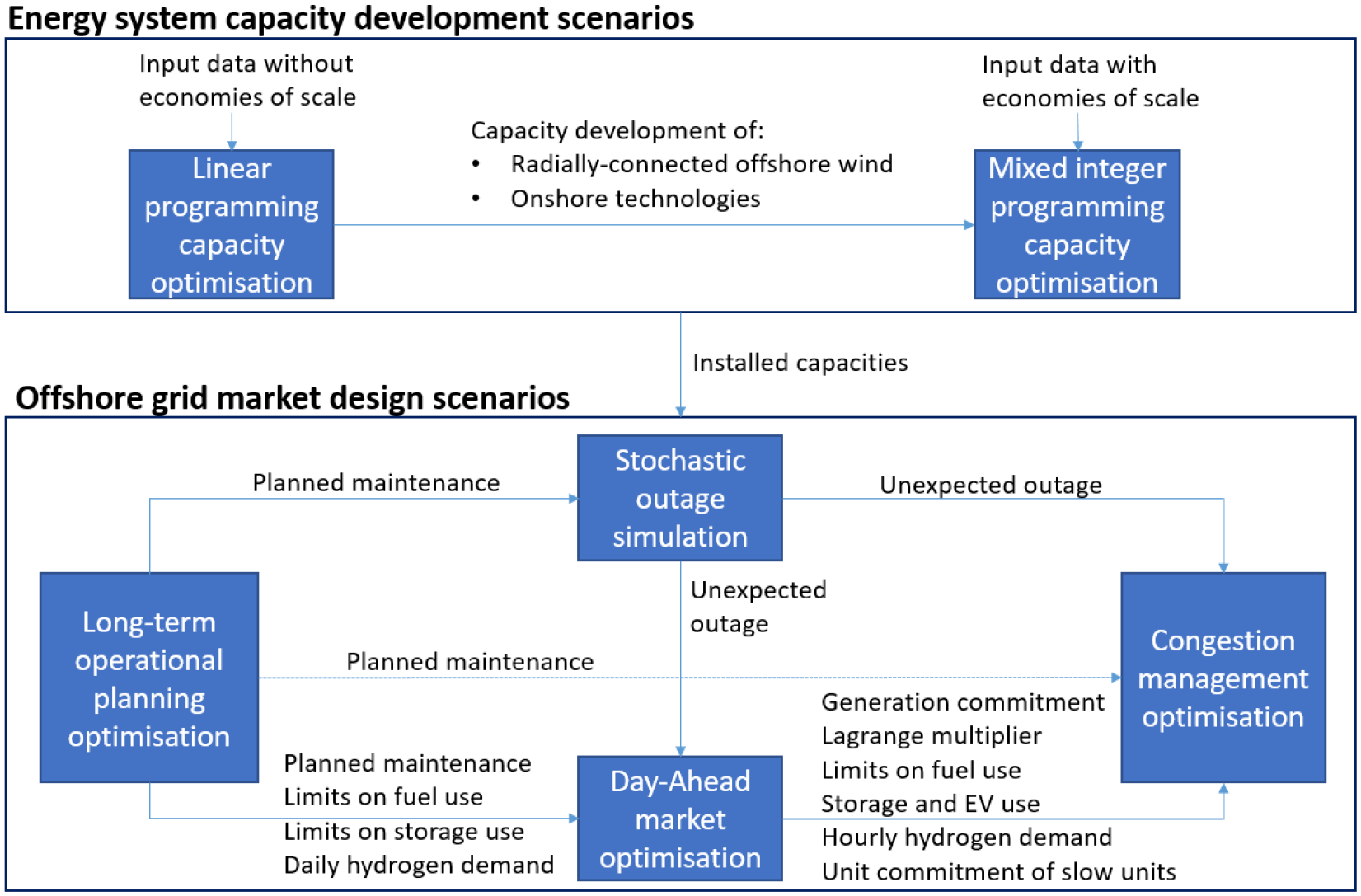
Optimisation sequence and input/output flow applied to derive the scenarios of this paper. The optimisation sequence used for the capacity development scenarios is described in Section 2.2.1, and the one used for the market design scenarios is described in Section 2.2.2. EV stands for electric vehicles.

Table 2:

Main features of the model used in the different optimisations performed in the paper. ONP stands for offshore nodal pricing, OZP for offshore zonal pricing, NoOP for no offshore pricing, LP for linear programming, MIP for mixed integer programming, and RMIP for relaxed mixed integer programming. The stochastic outage simulation is not described here because it is not an optimisation model, but a simulation one.

Name of the optimisation	Purpose of the optimisation	Market designs simulated	Temporal foresight	Time slices of each year simulated	Economies of scale related to investments	Unit commitment variables and constraints	Solver used
Linear programming capacity optimisation	Optimise installed capacities	ONP	2 years	192 representative hours	Not included	Not included	LP
Mixed integer programming capacity optimisation	Optimise installed capacities in offshore grids	ONP	2 years	192 representative hours	Included	Not included	MIP
Long-term operational planning optimisation	Optimise long-term operational decisions	ONP, OZP, NoOP	1 year	1-every-3 hours of the year	-	Included	RMIP
Day-ahead market optimisation	Simulate day-ahead markets	ONP, OZP, NoOP	1 day	All hours of the year	-	Included	MIP
Congestion management optimisation	Simulate congestion management	ONP	1 hour	All hours of the year	-	Included	MIP

First, we derive energy system capacity development scenarios towards 2050, where off-

shore grid development can take place. For this purpose, two main scenarios are created: BASE and OFFH2.

The BASE scenario allows H₂ generation anywhere and lets the model decide on optimal on- and offshore capacities for H₂ generation.

Compared to BASE, the scenario OFFH2 corresponds to a scenario where there is a strong will to incentivise the development of offshore H₂ generation. In terms of modelling, the only difference between the two scenarios is that in the OFFH2 scenario, investments in electrolysers located onshore are not allowed, meaning that all H₂ generation is moved offshore (integrated as part of offshore grids). The motivation for this second scenario relates to the possible future scenario, in which large capacities of electrolysers are beneficial to be deployed offshore as part of the many planned projects for “energy islands” and offshore energy hubs. We study this dedicated offshore hydrogen scenario to investigate the impact of such a configuration of hydrogen generation in the European energy system on the different offshore market design options.

These two scenarios can lead to very different configurations, use and purpose of the offshore grids, and therefore, can influence the impact of different offshore market configurations. Details about how the optimisations for these capacity development scenarios are performed can be found in Section 2.2.1.

After having derived the capacity development scenarios, we simulate the impact of implementing different day-ahead offshore electricity market designs in each of them. Three offshore electricity market design options are modelled (see Figure 5 for an illustration):

Figure 5:

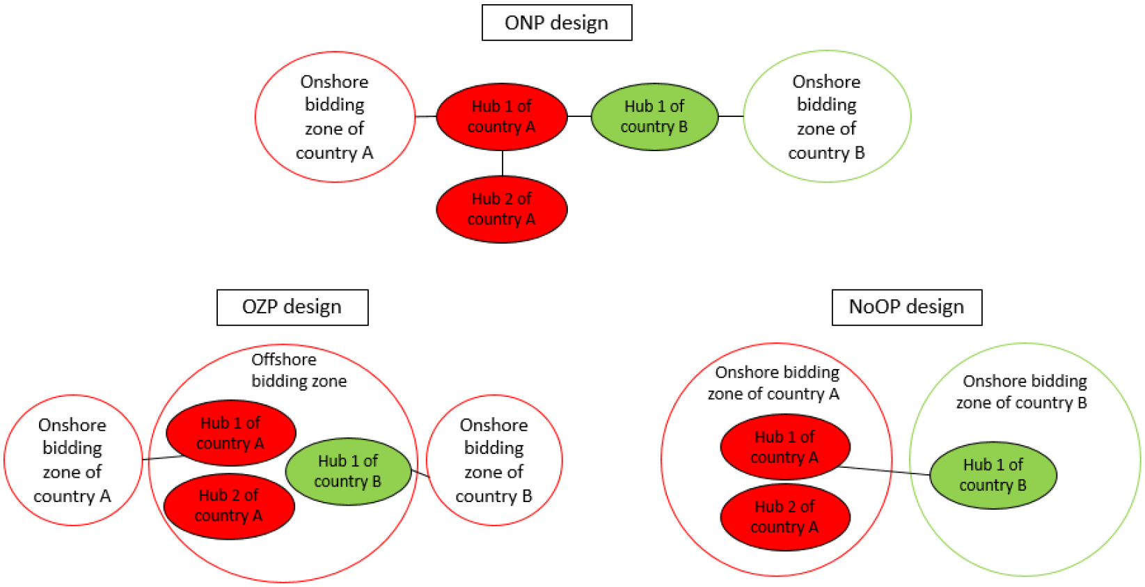
Offshore market designs investigated in the paper. Black lines correspond to the electric interconnectors that are not ignored when using the different market configurations. ONP stands for offshore nodal pricing, OZP for offshore zonal pricing, and NoOP for no offshore pricing.

ONP (offshore nodal pricing): In this market design, one hub represents one node and each hub/node corresponds to a bidding zone.

OZP (offshore zonal pricing): In this market design, all hubs are assumed to form a unique offshore bidding zone. To model this design, we ignore hub-to-hub electricity transmission capacity constraints and losses.

NoOP (no offshore pricing): In this market design, hubs are assumed to be part of one onshore bidding zone of the country they belong to. The corresponding onshore region is the closest one that belongs to the same country, except for Germany, for which the western region (DE-W) is used for simplicity. To model this design, electricity transmission capacity constraints and losses of hub-to-hub electricity interconnectors of hubs that belong to the same corresponding onshore bidding zone, and of hub-to-corresponding onshore bidding zone, are ignored.

Zonal market design is used for onshore regions in all the runs.

After simulating day-ahead markets with different offshore electricity market designs, we then simulate the required congestion management that transmission system operators perform to make sure a feasible dispatch of the units takes place in real time, which is a consequence of having ignored some of the offshore grid electricity transmission lines in the zonal market configurations.

Details about how these market scenarios are created can be found in Section 2.2.2.

2.2.1 Generation capacity development scenarios

Each capacity development scenario is obtained by performing two consecutive optimisations. The first optimisation uses linear programming (LP) and the second optimisation uses mixed integer programming (MIP). The objective of the LP optimisation is to analyse the competition of all the technologies included in the model (including the development of offshore grids), whereas the objective of the MIP optimisation is to model economies of scale of offshore grids to avoid unrealistically small investments in offshore grids. The approach is based on Gea-Bermúdez et al. (2020). In the MIP optimisation, investments, decommissioning, and/or mothballing of almost all technologies are forced from the LP optimisation to reduce calculation time and make the problem solution feasible. The exceptions are: hub-connected units (electrolysers, H₂ storage, OWPP, and fuel cells), hub platforms, and offshore H₂ pipes and offshore transmission lines in the North Sea. Economies of scale are modelled in offshore electricity transmission lines, offshore H₂ pipes and offshore hubs. Because of including all the potential offshore electricity interconnectors in the optimisations, the offshore configuration used in these runs is therefore equivalent to using a ONP market design. This approach aims to find the least-cost offshore grid development for the system, i.e. the one that maximises social welfare, and at the same time, facilitates the comparison of the operation of the system under different offshore electricity market designs, since the same installed capacities are used in the different market design scenarios run. In reality, the actual market design will be the one driving investment decisions too. However, how market configurations impact the offshore capacity development of the system towards 2050 is another research question that is out of the scope of this paper.

Both MIP and LP optimisations are obtained using limited inter-temporal foresight with a two-year rolling horizon approach similar to Gea-Bermúdez et al. (2023). Since in this paper we run the years 2025, 2035, and 2045, the approach considered translates into optimising 2025 with perfect foresight of 2035, save investment decisions of the year 2025, and then optimise 2035 with perfect foresight of 2045. Therefore, each investment runs includes two subruns: 2025–2035, and 2035–2045. In these runs, the meaning of seasons and terms are weeks and hours of the week, respectively.

Due to the complexity of the MIP and LP runs, only a limited amount of time steps are used in these runs. The time steps are selected with the approach described in Gea-Bermúdez et al. (2020). In the LP and MIP runs, we use 8 weeks that are spread over the year, the days of the week Thursday, Friday, Saturday, and 1 every 3 hours of each of those days, resulting in 192 time slices per year. Using the methodology described in Gea-Bermúdez et al. (2020), the time series are scaled using probability integral transformations to maintain the annual statistical properties of the original hourly time series. Weather data from several years (40 years for wind and solar PV) is used in the scaling of the time series to improve VRE representation in the reduced amount of time steps used. EV profiles and seasonal hydro inflow are scaled in a different way though for simplicity due to their modelling being different to the rest of the time series: EV profiles correspond to the average of three-consecutive-hour time steps, and seasonal hydro inflow is linearly scaled with respect to average annual inflow.

Annual average availability of the generation and storage units, as well as all type of energy

transmission in the model (electricity, H₂, and district heating) is assumed for all the time steps used.

Unit commitment constraints, and related variables and costs are not considered in these runs to simplify the problem and make the MIP computational feasible. The impact of this simplification on results should not be high considering the high number of flexibility options that are included in the model (Poncelet et al., 2020).

The key output from this set of optimisations is investments, mothballing, decommissioning, and peak regional H₂ demand to generate synthetic fuels for the transport sector towards 2050.

These results are then used as input in the offshore grid market design scenarios.

2.2.2 Scenarios for offshore grid market design

To derive the impact of having different offshore market designs in each of the energy system capacity development scenarios, we perform the following consecutive optimisations/simulations: long-term operational planning optimisation, stochastic outage simulation, day-ahead market optimisation, and congestion management optimisation. The method is inspired (and expanded) from the one used in the scenarios of Gea-Bermúdez et al. (2021).

A large amount of back-up expensive-to-operate fast units (gas turbines for the electricity sector) are added to the scenarios to avoid unmet load due to lack of generation capacity in the system. The lack of generation capacity can be a consequence of having used a reduced amount of time steps when performing the capacity development optimisations. As shown by Gea-Bermúdez et al. (2023), the importance of this back-up capacity is likely to be very small in terms of total generation, and non-negligible in terms of capacity. The investment costs and fixed costs of these back-up units are not reported in the results of the paper based on the assumption that the optimal installed capacity of these units would not be highly affected by the actual market design, and that would mainly be driven by security of supply standards.

Long-term operational planning optimisation: The first step is to optimise long-term operational decisions that influence the dispatch of the units involved in day-ahead markets by running optimisations with perfect foresight for all the time steps withing a year and for each year in the different capacity development scenarios. Such decisions correspond to the use of storage along the year, the use of fuels with annual limits, the planned maintenance of generation and storage units along the year, and the distribution of H₂ demand to generate synthetic fuels for the transport sector. Planned maintenance is assumed to have to take place during consecutive time steps (more information on the method can be found in Gea-Bermúdez et al., 2021). In this optimisation, seasons represent days, and terms are assumed to be the hours of the day. Due to the complexity of the run, only one of every three hours of each day of the year is used as time step. Time series are not scaled, except for EV profiles, which are the average of three-consecutive-hour time steps.

The objective function of these runs is to minimise the variable operational costs of each analysed year. The years are optimised in parallel to speed up the runs.

Generation units are assumed to have full availability, whereas all type of energy transmission in the model (electricity, H₂, and district heating) are assumed to have annual average availability in each time step. Unit commitment constraints (minimum fuel generation, minimum time on/ off, and ramping limitations), and related variables and costs are considered in this runs. However, to reduce the complexity of the optimisation, the commitments of the units in the different seasons are not linked (i.e. the on/off status of one season disregards what happened in previous seasons). To help computational speed, we relax integer variables. Relaxing the integer variables is likely not to have a significant impact on the key output from these runs (Gea-Bermúdez et al., 2021).

In these runs, offshore grids are modelled using the three different market designs for each capacity development scenario to reflect that optimal long-term operational decisions are likely to be affected by the actual day-ahead offshore electricity market design.

Stochastic outage simulation: The second step is to simulate stochastic outages for each hour of each year of the energy system capacity development scenarios. Part of the unavailability during the year of the units in the system is unexpected and thus uncertain. To capture this in the model, we perform Monte Carlo simulations for each generation and storage unit of the system individually to simulate hourly stochastic outages. This approach is not applied to VRE units, since their time series already account for the stochastic availability. More information on the method can be found in Gea-Bermúdez et al. (2021). The years are simulated in parallel to speed up the runs.

Day-ahead market optimisation: The third step is to simulate the operation of day-ahead markets (market clearing) using total system cost minimisation for each year and each of the energy system capacity development scenarios to derive, among other things, day-ahead prices and energy generation commitment of the units. In this optimisation, seasons mean days, and terms include the 24 hours of the day. To simulate the operations on the day-ahead market, the optimisations are performed with a seasonal rolling horizon approach of one day of foresight, assuming this market takes place 24 hours before delivery.

The objective function of these runs is to minimise the variable operational costs (fuel

costs, CO₂ tax, etc.) of each day, starting with the optimisation of the first day of the year and ending with the last one. The years are optimised in parallel to speed up the runs.

Unit commitment constraints (minimum fuel generation, minimum time on/off, and ramping limitations) and related variables and costs are considered in this run. The commitment of the units in the different seasons are linked, which means that the on/off status in one season is limited by the on/off status in previous seasons.

From the corresponding stochastic outage simulation, this run uses as input the hourly stochastic outages.

Based on the results of the corresponding long-term operational optimisation, the dayahead optimisation run sets limits to the seasonal use of fuels with annual restrictions, forces the energy content of storage units at the beginning of each day and the planned maintenance during the year, and forces the total daily H₂ demand to generate synthetic fuels for the transport sector, although its distribution along the day is optimised.

Congestion management optimisation: The last step is to simulate the required congestion management that transmission system operators do to make sure that a feasible dispatch of the units takes place in real time, which necessitates from having ignored some of the offshore grid electricity transmission line constraints in day-ahead market runs.

In these congestion management runs, we use the ONP market design configuration to make sure the actual transmission lines are considered. In these optimisations, seasons mean hours, and terms include just one hour.

To simulate the behaviour of congestion management markets, the optimisations are performed using a seasonal rolling horizon approach of one hour of foresight, assuming this market takes place one hour before delivery.

A penalty (additional cost) is added to the objective function to reflect the payment that transmission system operators would need to make to the units that have been asked to generate less energy than the commitments made in the day-ahead market, i.e. the constrained off payment. The value of such penalty for each year y, technology t, output commodity (electricity, heat, H₂, or SNG) c, and hour h is the Lagrange multiplier $L_{y, h, t, c}^{D a y A h e a d}$ of the maximum hourly generation equation, i.e. the generation of each technology in each hour must be lower or equal than its available installed capacity in that hour, of the corresponding day-ahead market optimisation. The penalty can be interpreted as the marginal profit of the unit, and hence, is the price required to make the unit indifferent to generate less than committed in day-ahead markets.

The resulting objective function in the model for the congestion management runs is Equation 3, which minimises, in each hour h, the total variable operating and maintenance costs of the system $c_{y, h}^{v o m}$ (fuel costs, CO₂ tax, etc.), and the total penalty $c_{y, h}^{p e n a l t y}$ . The first optimisation performed is the first hour of the year, and the last one the last hour of the year. The years are optimised in parallel to speed up the runs.

\min_{c_{y, h}^{v o m}, c_{y, h}^{p e n a l t y}} c_{y, h}^{v o m} + c_{y, h}^{p e n a l t y}

(3)

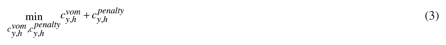
The total penalty is calculated using the non-negative variable $g_{y, h, t, c}^{d o w n}$ , which is modelled using Equations 4 and 5. Such variable only has an impact on costs if the corresponding Lagrange multiplier $L_{y, h, t, c}^{D a y A h e a d}$ is higher than 0 and the unit’s generation after congestion management $g_{y, h, t, c}^{A t e r C o n g M a n a g}$ is lower than its corresponding generation commitment in the day-ahead market $G_{y, h, t, c}^{D a y A h e a d}$ .

c_{y, h}^{p e n a l t y} = \sum_{c, t} (g_{y, h, t, c}^{d o w n} \cdot L_{y, h, t, c}^{D a y A h e a d})

(4)

g_{y, h, t, c}^{A t e r C o n g M a n a g} \geq G_{y, h, t, c}^{D a y A h e a d} - g_{y, h, t, c}^{d o w n} \forall t, \forall c

(5)

Unit commitment constraints (minimum fuel generation, minimum time on/off, and ramping limitations), and related variables and costs are considered in this run. The commitment of the units in the different seasons are linked, which means that the on/off status in one season is limited by the on/off status in previous seasons. The on/off commitment of the units whose technical characteristics are assumed to prevent them from being able to generate from 0 to full capacity in 1 hour is forced to be the same as the one from the corresponding day-ahead market optimisation. The rest of the units are allowed to deviate if found optimal.

The use of all sort of units with storage (including EVs) is forced from the corresponding day-ahead market optimisation. The hourly H₂ demand for synthetic fuel generation for the transport sector is also forced to be the same as the one from the corresponding day-ahead market optimisation. Additionally, the use of fuels with annual restrictions is also limited in each season from the corresponding day-ahead market optimisation.

This run uses as input the stochastic outage from the corresponding stochastic outage simulation, and forces the planned maintenance during the year from the corresponding long-term operational planning optimisation.

In summary, this run represents an energy system where the system operator aims to minimise costs, has one-hour foresight, has control of all the units in the system, and can modify the generation of the units (and the on/off status of relatively fast units) as long as it compensates them so their final profit is not lower than the one expected from the actions on the day-ahead markets.

3. Results

This section summarises and discusses the results obtained from the different optimisations. It focuses first on the two capacity expansion scenarios and continues with the answers to the research question, i.e. the impact of different offshore zonal market configurations on prices and system costs. The section also includes a critical reflection on key modelling assumptions. All monetary values are provided in €2016.

3.1 Energy system capacity development scenarios

The energy system of both scenarios (BASE and OFFH2²) sees a large increase of electricity demand towards 2050 in both scenarios (Table 3), which is linked to strong sector coupling between electricity, heat and transport sectors. Sector coupling increases demand, but also the flexibility in the system. The increase in electricity demand, combined with the CO₂ tax assumptions and the significant cost reduction assumed for wind and solar PV technologies (Table 9) leads to high investments in wind and solar PV technologies, resulting in a large penetration of these technologies in the system (Table 3). In the capacity development runs, the share of wind and solar PV generation within the total electricity demand by 2045 is 83% in scenario BASE and 85% in scenario OFFH2. As a result of the strong VRE penetration, the green house gas (GHG) emissions in the energy sector are considerably reduced: by 2025, 2035, and 2045 GHG emissions represent 41%, 12%, 2% respectively of 1990 levels in both scenarios.³ Strong electricity and H₂ transmission development also takes place in both scenarios to provide flexibility to the system.

Table 3:

Summary of key energy system results per year and scenario.

Scenario	Electricity demand (TWh)			Hub-connected offshore wind generation (TWh)			Share of wind and solar PV generation in total electricity demand			Green house gas emissions in the energy sector relative to 1990 levels
	2025	2035	2045	2025	2035	2045	2025	2035	2045	2025	2035	2045
BASE	2128	2148	5250	-	353	489	43%	75%	83%	41%	12%	2%
OFFH2	2124	3033	5187	-	704	1384	43%	75%	85%	41%	12%	2%

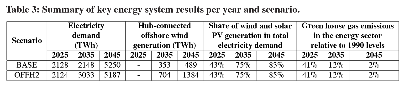
The scenarios are therefore very similar in terms of annual electricity demand, annual emissions, and annual wind plus solar PV generation.

Part of the offshore wind development in the scenarios takes place in offshore grids. However, investments in hub-connected offshore wind only take place from 2035 onwards. This result is likely to be related to offshore wind being more expensive than other competitors like solar PV or onshore wind.

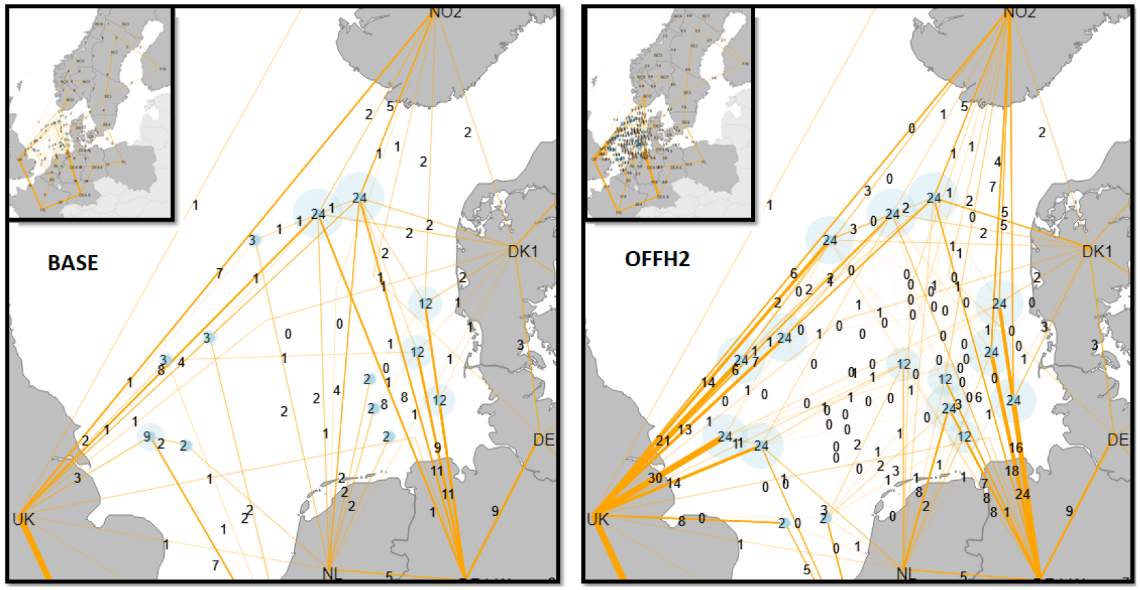
The development of the offshore grid is considerably different in the two studied scenarios (Figure 6 and Figure 7). In the BASE scenario, the installed hub-connected offshore wind capacity is 79.6 GW by 2035 and 109.5 GW by 2045, whereas in the OFFH2 scenario it is 155.6GW by 2035 and 304.4 GW by 2045 (Table 3). The total hub-to-shore connections are roughly 5–10 times the total hub-to-hub capacity in the different scenarios. In the capacity development scenarios, these installed capacities lead to hub-connected wind generation of 353 TWh by 2035 and 489 TWh by 2045 in the BASE scenario, and 704 TWh by 2035 and 1384 TWhW by 2045 in the OFFH2 scenario, i.e. considerably larger generation in scenario OFFH2.

Figure 6:

Transmission map of the studied North Sea region for each scenario in 2045. The space that hub-connected wind farms would require are depicted in the light blue circles, whereas the total hub-connected wind farm capacity is shown as numbers in the middle of such circles, which represents the location of the hub. Transmission lines, (i.e. interconnectors) are depicted in orange. The unit for all the numbers is GW. All numbers have been rounded to the unit. The entire energy system modelled is shown in the upper left corner of each figure.

Figure 7:

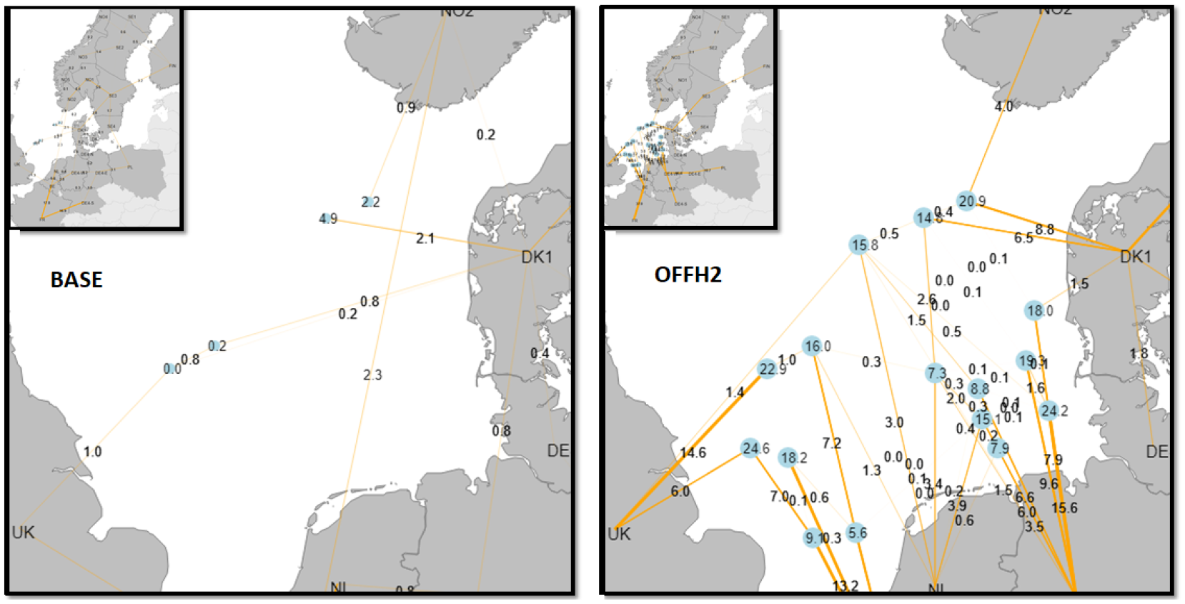
Hydrogen grid by 2045 and scenario. Hubs with electrolyser capacity are depicted as blue dots and hydrogen pipes as yellow lines. The hubs without electrolyser capacity are not shown. The total electrolyser capacity in each hub is the number that is in the middle of the blue dots, whereas the numbers that are on top of the orange lines correspond to the hydrogen pipe capacity. The unit for all the numbers is GW. The numbers have been rounded to the first decimal. The entire energy system modelled is shown in the upper left corner of each figure.

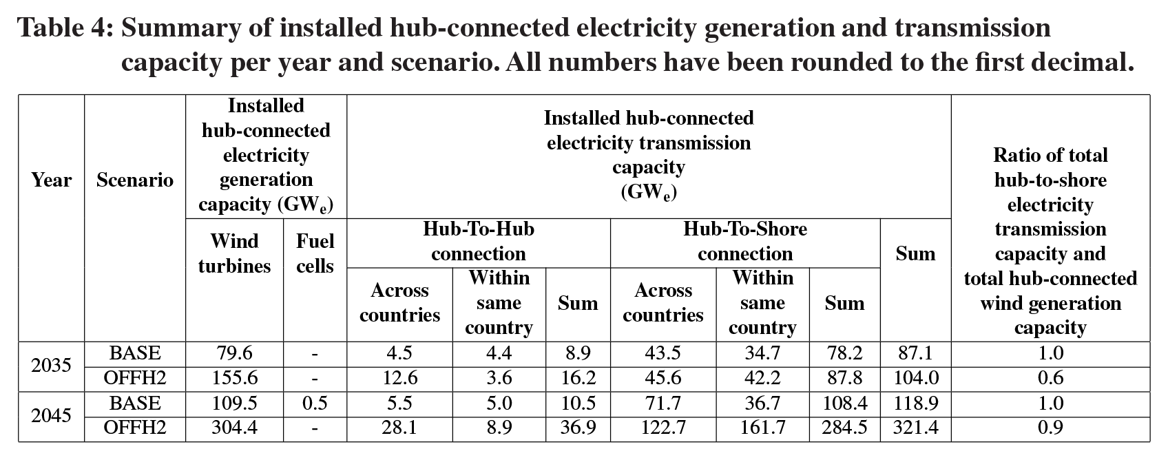
The level of H₂ generation taking place in the hubs is very different between the two scenarios. In the BASE scenario, most of the electrolysers are built onshore, and therefore only a small share of the total H₂ generation from electrolysers takes place offshore (0.1% by 2035, and 1.5% by 2045). In the OFFH2 scenario, the offshore electrolyser deployment (Table 5) is considerably larger due to the assumptions, since all H₂ generation is forced to take place offshore. The reason for offshore H₂ having such a small role in the overall H₂ generation in scenario BASE is because producing H₂ onshore is found more cost-effective than offshore. This result is linked to solar PV generation patterns that lead to low electricity prices in the middle of the day, high electricity transmission expansion, and high use of H₂ storage.

The different role that offshore H₂ generation plays in the scenarios has a strong influence on the design of the electricity infrastructure of offshore grids. For instance, the ratio of hub-connected electricity transmission capacity and hub-connected wind capacity is around 1 in the BASE scenario (Table 4), which means that the offshore grid is likely to be able to transport almost all of the offshore wind generation onshore in every time step. However, in the OFFH2 scenario this ratio is lower than 1 in both years, suggesting that not all hub-connected wind generation can be sent onshore, and therefore, part of the generation needs to be consumed in the electrolysers of the hubs, or curtailed. This is highly linked to having a large amount of electrolysers in the hubs, which leads to finding optimal to design the electrical interconnectors of a hub with lower electrical capacity than the installed hub-connected offshore wind capacity in that hub. This ratio is key when analysing the importance of ignoring hub-to-shore transmission lines when using market design NoOP.

Table 4:

Summary of installed hub-connected electricity generation and transmission capacity per year and scenario. All numbers have been rounded to the first decimal.

Year	Scenario	Installed hub-connected electricity generation capacity (GW_e)		Installed hub-connected electricity transmission capacity (GW_e)							Ratio of total hub-to-shore electricity transmission capacity and total hub-connected wind generation capacity
		Wind turbines	Fuel cells	Hub-To-Hub connection			Hub-To-Shore connection			Sum
		Wind turbines	Fuel cells	Across countries	Within same country	Sum	Across countries	Within same country	Sum	Sum
2035	BASE	79.6	-	4.5	4.4	8.9	43.5	34.7	78.2	87.1	1.0
2035	OFFH2	155.6	-	12.6	3.6	16.2	45.6	42.2	87.8	104.0	0.6
2045	BASE	109.5	0.5	5.5	5.0	10.5	71.7	36.7	108.4	118.9	1.0
2045	OFFH2	304.4	-	28.1	8.9	36.9	122.7	161.7	284.5	321.4	0.9

Table 5:

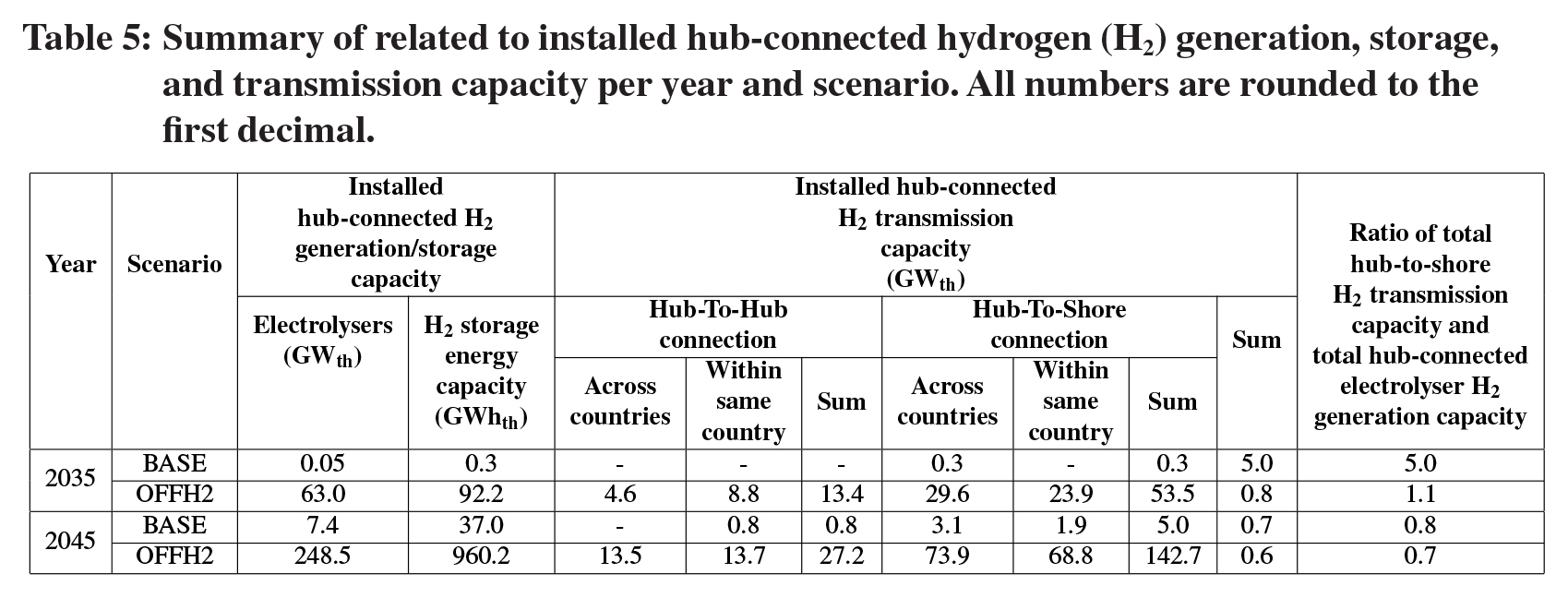
Summary of related to installed hub-connected hydrogen (H₂) generation, storage, and transmission capacity per year and scenario. All numbers are rounded to the first decimal.

Year	Scenario	Installed hub-connected H₂ generation/storage capacity		Installed hub-connected H₂ transmission capacity (GW_th)							Ratio of total hub-to-shore H₂ transmission capacity and total hub-connected electrolyser H₂ generation capacity
		Electrolysers (GW_th)	H₂ storage energy capacity (GWh_th)	Hub-To-Hub connection			Hub-To-Shore connection			Sum
		Electrolysers (GW_th)	H₂ storage energy capacity (GWh_th)	Across countries	Within same country	Sum	Across countries	Within same country	Sum	Sum
2035	BASE	0.05	0.3	-	-	-	0.3	-	0.3	5.0	5.0
2035	OFFH2	63.0	92.2	4.6	8.8	13.4	29.6	23.9	53.5	0.8	1.1
2045	BASE	7.4	37.0	-	0.8	0.8	3.1	1.9	5.0	0.7	0.8
2045	OFFH2	248.5	960.2	13.5	13.7	27.2	73.9	68.8	142.7	0.6	0.7

In scenario BASE, the installed electricity interconnection capacity of each hub both in 2035 and 2045 tends to be at least of the size of the installed wind capacity in the hub (Figure 8). In scenario OFFH2, by 2035 the ratio of installed electricity intercconection and wind capacity in the hubs tends to be lower than 1, and around 1 by 2045. This is a consequence of the high installed electrolyser capacity in the hubs in scenario OFFH2. In scenario OFFH2 by 2035, the installed electrolyser capacity in each hub is higher than the installed wind capacity in it (electrolyser to wind capacity ratio higher than 1), which suggests that H₂ generation in the hubs is likely to be highly dependent on electricity coming from other regions (onshore or offshore) in this year. By 2045 in scenario OFFH2 and compared to 2035, the electrolyser to wind capacity ratio decreases whereas the interconnector to wind capacity in the hubs increases. This suggests that hubs are more interconnected, but at the same time, more capable of satisfying their H₂ demand. Overall, the results suggest that in both scenarios hub-connected transmission is not only used to dispatch hub-connected offshore wind generation, but also acts as interconnectors between regions.

Figure 8:

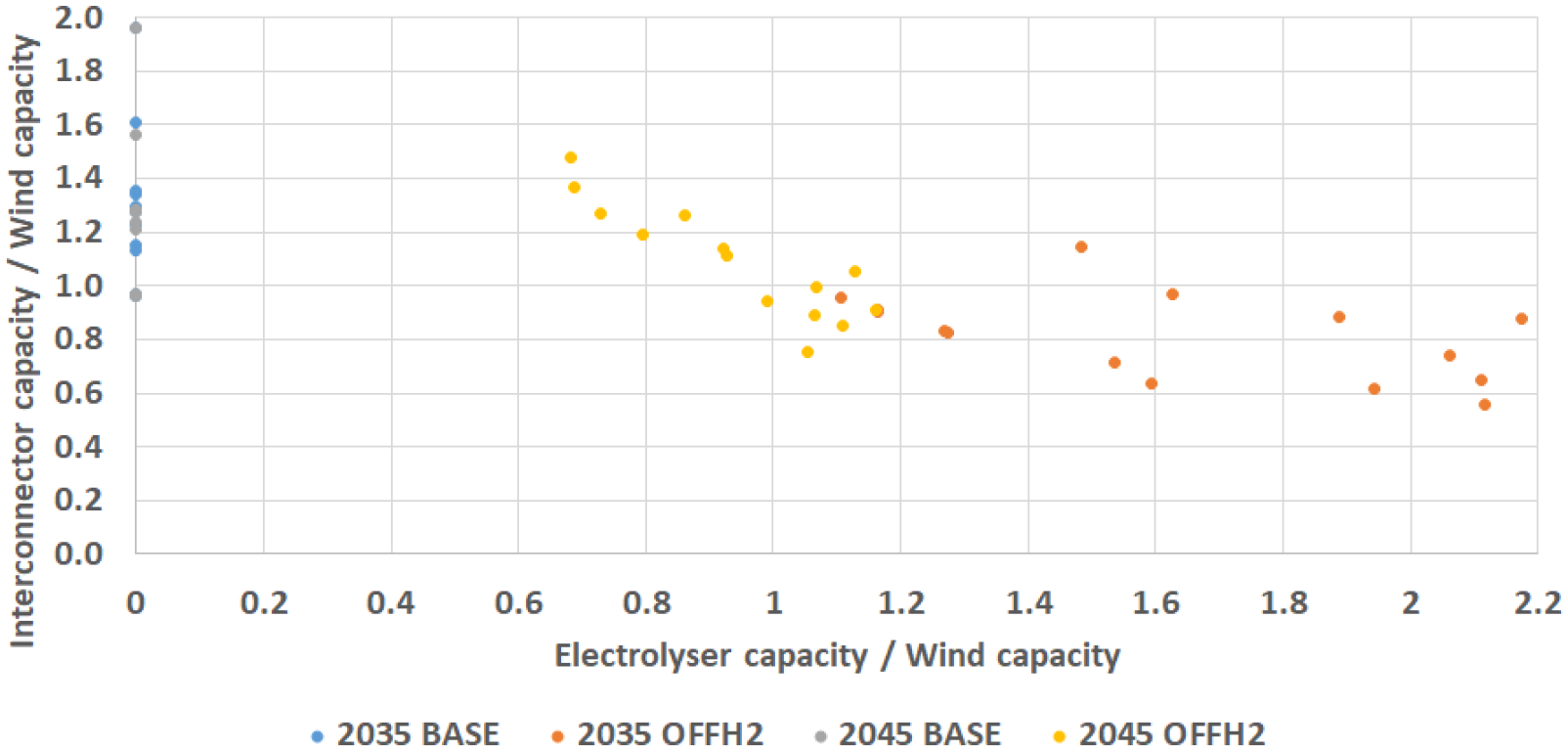
Ratio of aggregated electricity interconnector capacity and installed wind capacity in each hub versus ratio of installed electrolyser electricity input capacity and wind capacity in each hub per scenario and year. Each dot corresponds to an offshore hub. The aggregated electricity interconnector capacity of each hub is calculated by adding all the electricity interconnectors connected to that hub. The y axis has been limited to 2, and the x axis to 2.2 to show the most representative values.

The two scenarios, therefore, show different offshore grid configurations that are likely to be relevant when investigating the impact of the electricity offshore market design towards 2050.

3.2 Impact of offshore grid electricity market design

The results show that different offshore market designs have a significant influence on the energy system towards 2050.⁴ The impact on day-ahead markets, and on congestion management is presented below. For the sake of space limitations, we focus the analysis on the electricity side.

3.2.1 Impact on day-ahead markets

The impact of the offshore grid electricity market design on the average day-ahead electricity prices and on the average day-ahead H₂ prices (Table 6) is highly dependent on the year, region and capacity development scenario. In the studied years of the BASE scenario, in the hubs the difference between average prices of alternative market configurations and the ONP market design ranges between −1.0 and 2.7 €/MWh for electricity, and –1.6 and 0.9 €/MWh for H₂. In the OFFH2 scenario, in the hubs the difference between average prices of alternative market configurations and the ONP market design ranges between –1.4 and 2.7 €/MWh for electricity, and –1.3 and 8.6 €/ MWh for H₂.

Table 6:

Time-weighted average electricity and hydrogen prices in the offshore hubs of each country per year, scenario, and offshore market design. Values for electricity are only shown if there is electricity generation capacity or electricity interconnectors in the hubs, whereas values for hydrogen are only shown if there is hydrogen generation capacity or hydrogen interconnectors in the offshore hubs. ONP stands for offshore nodal pricing, OZP for offshore zonal pricing, and NoOP for no offshore pricing. All numbers are rounded to the first decimal.

Year	Scenario	Country where the offshore hubs are located	Average electricity price (in brackets difference with respect to corresponding onshore region) (=C/MWh)			Average hydrogen price (in brackets difference with respect to corresponding onshore region) (=C/MWh)
Year	Scenario	Country where the offshore hubs are located	ONP	OZP	NoOP	ONP	OZP	NoOP
2035	BASE	Norway	35.2 ( -0.7 )	37.9 ( 0.5 )	36.5 ( 0.0 )	52.9 ( -0.1 )	53.7 ( -0.1 )	53.9 ( -0.1 )
		Denmark	38.0 ( -0.4 )	37.9 ( -0.3 )	38.6 ( 0.0 )	-	-	-
		Germany	39.2 ( -1.1 )	37.9 ( -1.8 )	40.0 ( 0.0 )	-	-	-
		Netherlands	-	-	-	-	-	-
		United Kingdom	35.9 ( -2.7 )	37.9 ( -1.5 )	38.4 ( 0.0 )	52.9 ( -3.7 )	53.6 ( -5.2 )	53.9 ( -2.8 )
	OFFH2	Norway	36.7 ( -0.5 )	38.7 ( 1.2 )	38.5 ( 0.0 )	63.6 ( -2.3 )	66.2 ( -3.5 )	64.3 ( -2.7 )
		Denmark	38.3 ( -0.2 )	38.7 ( 0.3 )	39.5 ( 0.0 )	64.0 ( -2.9 )	66.2 ( -3.5 )	65.8 ( -1.3 )
		Germany	39.0 ( -2.4 )	38.7 ( -2.0 )	40.4 ( 0.0 )	63.9 ( -5.1 )	66.3 ( -3.7 )	66.9 ( -4.3 )
		Netherlands	39.7 ( -2.3 )	38.7 ( -2.3 )	41.0 ( 0.0 )	66.3 ( -11.9 )	66.6 ( -7.6 )	67.7 ( -6.5 )
		United Kingdom	36.9 ( -2.7 )	38.7 ( -0.7 )	39.3 ( 0.0 )	66.3 ( -15.1 )	67.3 ( -6.6 )	67.9 ( -7.0 )
2045	BASE	Norway	28.9 ( -1.3 )	31.8 ( 0.7 )	30.6 ( 0.0 )	38.3 ( -0.6 )	38.6 ( -0.5 )	38.6 ( -0.3 )
		Denmark	32.1 ( -1.1 )	31.8 ( -1.1 )	32.9 ( 0.0 )	-	-	-
		Germany	33.4 ( -0.8 )	31.8 ( -1.8 )	33.9 ( 0.0 )	-	-	-
		Netherlands	-	-	-	-	-	-
		United Kingdom	29.2 ( -1.8 )	31.8 ( 0.2 )	31.3 ( 0.0 )	37.7 ( 1.9 )	38.5 ( 2.0 )	38.0 ( 2.3 )
	OFFH2	Norway	30.4 ( 1.4 )	30.6 ( 1.7 )	29.2 ( 0.0 )	45.1 ( -2.6 )	46.2 ( -1.4 )	45.4 ( -1.4 )
		Denmark	31.1 ( 0.3 )	30.6 ( 0.4 )	30.1 ( 0.0 )	45.8 ( -0.8 )	46.1 ( -1.7 )	45.6 ( -2.1 )
		Germany	31.5 ( -0.5 )	30.6 ( -0.5 )	30.6 ( 0.0 )	46.4 ( -1.6 )	46.2 ( -1.6 )	46.9 ( -1.2 )
		Netherlands	32.2 ( 0.1 )	30.6 ( -0.5 )	30.8 ( 0.0 )	47.3 ( -3.5 )	46.4 ( -0.9 )	47.5 ( -1.1 )
		United Kingdom	31.1 ( 0.8 )	30.6 ( 0.8 )	29.7 ( 0.0 )	46.3 ( -1.3 )	46.1 ( -1.6 )	46.9 ( -1.6 )

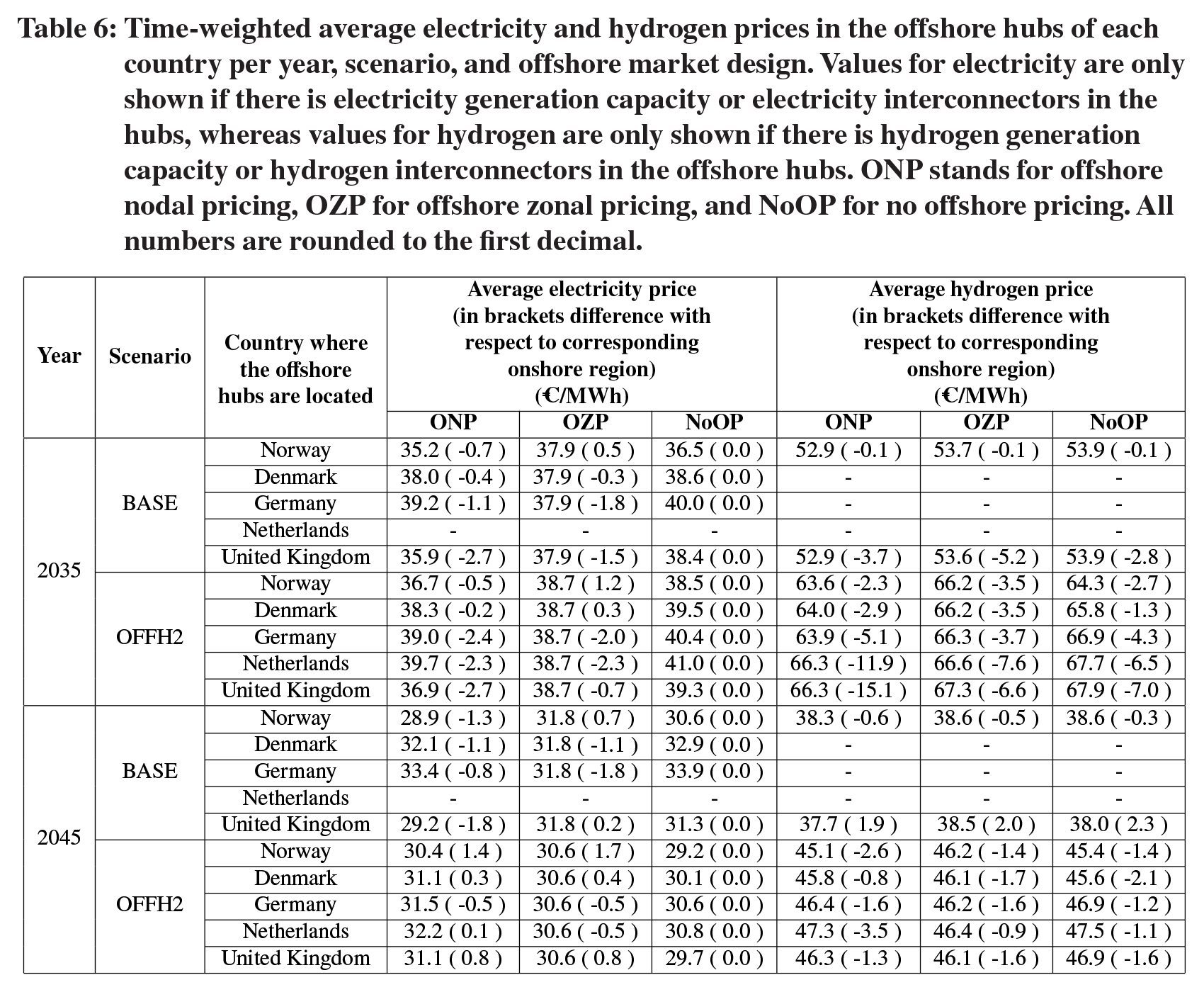
The average price difference of offshore hubs with their corresponding onshore region (Table 6) is highly dependent on the scenario and market design. Overall, average prices in the offshore hubs are lower than in their corresponding onshore regions, which is an expected result considering the higher likelihood of curtailment in the offshore hubs due to electricity line congestion. However, in a few cases the average prices in the offshore regions are higher than in their corresponding onshore region. The difference in electricity prices is overall limited, ranging from –2.7 to 1.7 €/MWh in the different scenarios and years, and considerably higher for H₂ prices, ranging from −15.1 to 2.3 €/MWh.

H₂ prices are likely to be highly linked to electricity prices, but may have been affected by H₂ pipeline congestion and H₂ storage. At the same time, electricity prices in the hubs may have been affected by H₂-related technologies, specially in scenario OFFH2, since all electrolysers are placed in the offshore hubs in this scenario. The magnitude of the impact is likely to be highly dependent on the installed generation, storage, and transmission capacities in each hub.

The analysis of the hourly distribution of the difference in electricity price of the offshore hubs with their corresponding onshore region shows that in most of the hours the difference is very small, which explains the limited average difference. This suggests that offshore prices are set by onshore prices in most of the hours (Figure 9). The analysis also shows that there is a higher number of hours with lower electricity price in the hubs than in their corresponding onshore region, which explains that the difference in average prices is generally negative. This result is most likely linked to curtailment taking place in the hubs due to electricity line congestion. 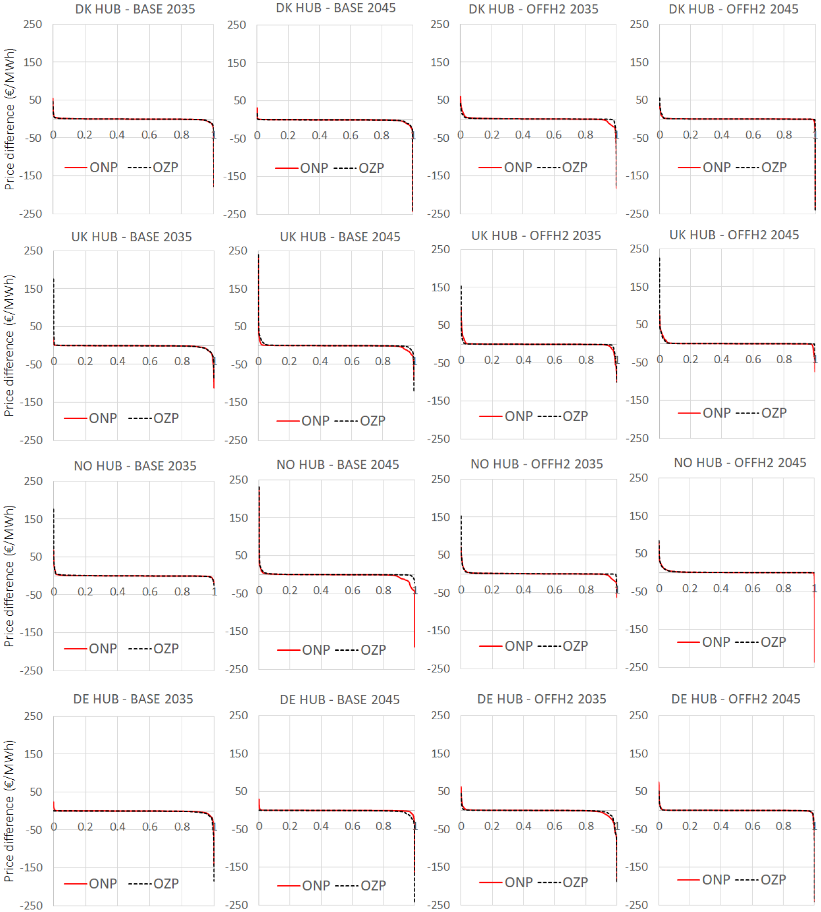Figure 9 also shows that, overall, when using market design ONP the number of hours with negative difference is higher than when using OZP market design, although this is not always the case. When using market design NoOP the difference in electricity price of the offshore hubs with their corresponding onshore region is zero because of having ignored all the relevant electricity transmission constraints.

Figure 9:

Ranked difference between electricity price in selected offshore hubs and the price in their corresponding onshore region per scenario, market design, and year. The difference when using market design NoOP (no offshore pricing) is 0, and hence, not shown. Only 4 out of 16 hubs are shown for illustrative purposes. ONP stands for offshore nodal pricing, OZP for offshore zonal pricing, DK for “Denmark, “UK” for the United Kingdom, NO for Norway, and “DE” for Germany.

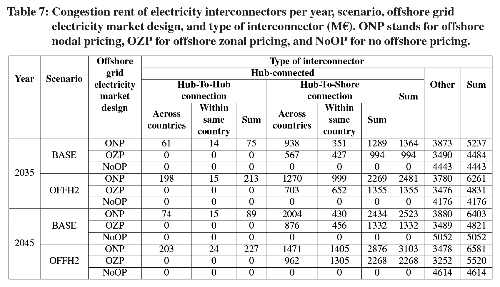
The offshore grid electricity market design has a significant impact on the congestion rent of electricity interconnectors (Table 7). In all the scenarios, the market design ONP is the one that leads to the highest total congestion rent. This is an expected result since this scenario can capture all line congestions. In hub-connected interconnectors, most of the congestion takes place in hubto-shore connections, which is linked to this group being the one with the highest share of installed hub-connected transmission capacity in the scenarios (Table 4). In scenario NoOP, the hubs are assumed to be part of the onshore bidding zone, and hence, hub-connected congestion rent is 0. The reduction in total congestion rent when using alternative market designs compared to ONP ranges from 752–2085 M€/year (14%–33%). In scenario BASE, both OZP and NoOP lead to similar congestion rent reduction, whereas for scenario OFFH2, the NoOP design leads to the highest reduction in 2035 and 2045. This suggests that hub-to-shore interconnectors are likely to be more binding in scenario OFFH2 than in scenario BASE. The congestion rent increases in both scenarios towards 2050, which is linked to higher transmission volumes. Towards 2050 the difference in congestion rent of alternative market designs with respect to market design ONP increases in the BASE scenario, and decreases in scenario OFFH2. Overall, these results are likely to be affected by the congestion of each interconnector when using the ONP market design. The magnitude of the congestion rent reduction when using alternative market designs is linked to the importance of the non-captured congestion of the interconnectors that have been ignored.

Table 7:

Congestion rent of electricity interconnectors per year, scenario, offshore grid electricity market design, and type of interconnector (M€). ONP stands for offshore nodal pricing, OZP for offshore zonal pricing, and NoOP for no offshore pricing.

Year	Scenario	Offshore grid electricity market design	Type of interconnector
			Hub-connected							Other	Sum
			Hub-To-Hub connection			Hub-To-Shore connection			Sum
			Across countries	Within same country	Sum	Across countries	Within same country	Sum	Sum
2035	BASE	ONP	61	14	75	938	351	1289	1364	3873	5237
		OZP	0	0	0	567	427	994	994	3490	4484
		NoOP	0	0	0	0	0	0	0	4443	4443
	OFFH2	ONP	198	15	213	1270	999	2269	2481	3780	6261
		OZP	0	0	0	703	652	1355	1355	3476	4831
		NoOP	0	0	0	0	0	0	0	4176	4176
2045	BASE	ONP	74	15	89	2004	430	2434	2523	3880	6403
		OZP	0	0	0	876	456	1332	1332	3489	4821
		NoOP	0	0	0	0	0	0	0	5052	5052
	OFFH2	ONP	203	24	227	1471	1405	2876	3103	3478	6581
		OZP	0	0	0	962	1305	2268	2268	3252	5520
		NoOP	0	0	0	0	0	0	0	4614	4614

In day-ahead markets alternative market designs to ONP lead to lower total curtailment (Table 10) from VRE technologies. Because of having ignored part of the transmission constraints when using alternative market designs to ONP, it is now possible to make use of cheaper energy coming from other VRE sources that, otherwise, would have probably been curtailed due to line congestion. By 2045 in scenario OFFH2, despite total curtailment being lower, when using NoOP market design the curtailment in the hubs is actually higher than when using the ONP market design. This can be explained by the large capacity of electricity interconnectors ignored (8.9+161.7 = 170.6 GW), which reduces congestion significantly, and the higher operational costs assumed for hub-connected offshore wind farms compared to other VRE technologies. When minimising costs, hub-connected offshore wind generation is likely to be curtailed before solar PV generation, for instance. These results highlight the importance of considering the synergies of highly-interconnected integrated energy systems.

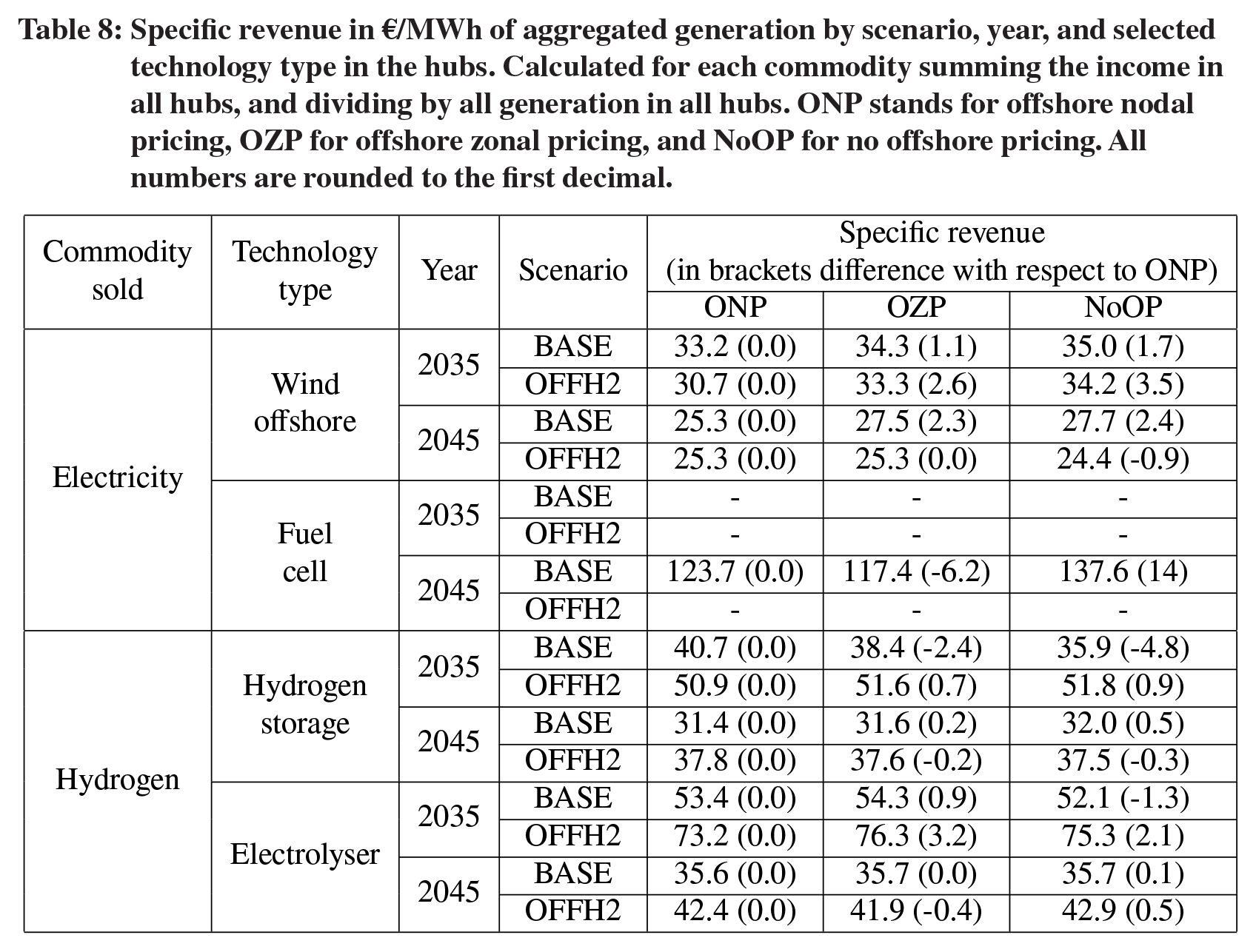
Specific revenues (also known as capture prices) of hub-connected technologies in dayahead markets are highly dependent on the technology studied, the capacity development scenario, the year, and the offshore market zone configuration (Table 8). The results for the different technologies are likely to be affected by the already discussed factors that influence average prices. Particularly, the difference in specific revenue of hub-connected offshore wind farms using alternative market design to ONP configuration is generally positive, suggesting that these units are likely to benefit if alternative market designs to ONP are implemented. Hub-connected wind farms only get lower specific revenue compared to ONP design when using NoOP in scenario OFFH2 by 2045, which is a result likely to be linked to the increase in hub-connected offshore wind curtailment experienced in this scenario (Table 10).

Table 8:

Specific revenue in €/MWh of aggregated generation by scenario, year, and selected technology type in the hubs. Calculated for each commodity summing the income in all hubs, and dividing by all generation in all hubs. ONP stands for offshore nodal pricing, OZP for offshore zonal pricing, and NoOP for no offshore pricing. All numbers are rounded to the first decimal.

Commodity sold	Technology type	Year	Scenario	Specific revenue (in brackets difference with respect to ONP)
Commodity sold	Technology type	Year	Scenario	ONP	OZP	NoOP
Electricity	Wind offshore	2035	BASE	33.2 (0.0)	34.3 (1.1)	35.0 (1.7)
		2035	OFFH2	30.7 (0.0)	33.3 (2.6)	34.2 (3.5)
		2045	BASE	25.3 (0.0)	27.5 (2.3)	27.7 (2.4)
		2045	OFFH2	25.3 (0.0)	25.3 (0.0)	24.4 (-0.9)
	Fuel cell	2035	BASE	-	-	-
		2035	OFFH2	-	-	-
		2045	BASE	123.7 (0.0)	117.4 (-6.2)	137.6 (14)
		2045	OFFH2	-	-	-
Hydrogen	Hydrogen storage	2035	BASE	40.7 (0.0)	38.4 (-2.4)	35.9 (-4.8)
		2035	OFFH2	50.9 (0.0)	51.6 (0.7)	51.8 (0.9)
		2045	BASE	31.4 (0.0)	31.6 (0.2)	32.0 (0.5)
		2045	OFFH2	37.8 (0.0)	37.6 (-0.2)	37.5 (-0.3)
	Electrolyser	2035	BASE	53.4 (0.0)	54.3 (0.9)	52.1 (-1.3)
		2035	OFFH2	73.2 (0.0)	76.3 (3.2)	75.3 (2.1)
		2045	BASE	35.6 (0.0)	35.7 (0.0)	35.7 (0.1)
		2045	OFFH2	42.4 (0.0)	41.9 (-0.4)	42.9 (0.5)

The total electricity demand in day-ahead markets is also affected by the market configura-

tion. The price-responsive electricity demand, part of it linked to sector coupling (EVs’ net charging, power to electricity, power to hydrogen, and power to synthetic natural gas) is highest when not using ONP configuration. This is an expected result linked to cheaper electricity generation system costs that are a result of having ignored part of the electricity grid and corresponding losses when not using ONP configuration. In the studied years, the price-responsive electricity demand difference of alternative market configurations with respect to ONP range from 0.2–2.6 TWh in scenario BASE, and from 2.8–8.4 TWh in scenario OFFH2.

These results suggest that the overall energy system development and the flexibility in it can have a large impact on the influence that offshore electricity market design has on congestion rents, the specific revenue of the hub-connected units as well as on the prices.

3.2.2 Impact on congestion management

In terms of variable operational system costs (Table 9) the results show that the offshore electricity market design that leads to the lowest final energy system costs is the ONP configuration in all the years and in both capacity development scenarios.

Table 9:

Operational system costs per year and scenario. Investment costs and fixed operational costs are not shown. ONP stands for offshore nodal pricing, OZP for offshore zonal pricing, NoOP for no offshore pricing, Constr. Off payment stands for constrained-off payments, and O&M costs for operation and maintenance. O&M costs includes in this table all variable costs (fuel cost, start-up cost, etc.), except the cost of the CO₂ tax. Operational costs from day-ahead markets should be interpreted as the cost the system would face if the operation of the units in real time was the same as the one committed in day-ahead markets. All numbers are rounded to the first decimal except constrained off payments, which have been rounded to the second decimal due to their order of magnitude being relatively low compared to the other values.

Year	Scenario	Offshore grid electricity market design in Day-ahead market	Day-Ahead variable operational cost (b=C)			Additional cost incurred in the energy system related to congestion management (b=C)				Final variable operational cost (b=C)
Year	Scenario	Offshore grid electricity market design in Day-ahead market	O&M cost	CO2 tax	Sum	O&M cost	CO2 tax	Constr. off payment	Sum	O&M cost	CO2 tax	Constr. off payment	Sum
2035	BASE	ONP	27.3	4.5	31.8	0.0	0.3	0.02	0.3	27.4	4.8	0.02	32.2
		OZP	27.1	4.4	31.6	0.4	0.5	0.04	0.9	27.5	4.9	0.04	32.4
		NoOP	27.2	4.5	31.7	0.2	0.4	0.02	0.6	27.5	4.8	0.02	32.3
	OFFH2	ONP	27.7	4.9	32.6	0.1	0.2	0.01	0.3	27.8	5.1	0.01	32.9
		OZP	27.5	4.7	32.3	0.6	0.6	0.06	1.3	28.2	5.3	0.06	33.6
		NoOP	27.5	4.5	32.0	1.0	0.8	0.33	2.1	28.5	5.3	0.33	34.2
2045	BASE	ONP	25.8	2.1	27.9	0.2	0.0	0.01	0.2	26.0	2.2	0.01	28.1
		OZP	25.6	2.1	27.7	0.7	0.3	0.02	1.0	26.3	2.4	0.02	28.7
		NoOP	25.6	2.1	27.7	0.6	0.2	0.02	0.8	26.2	2.3	0.02	28.6
	OFFH2	ONP	27.4	3.3	30.7	0.2	0.0	0.01	0.2	27.6	3.4	0.01	31.0
		OZP	26.9	3.0	30.0	1.5	1.0	0.04	2.6	28.5	4.0	0.04	32.5
		NoOP	26.8	2.9	29.7	1.3	0.8	0.04	2.2	28.1	3.8	0.04	31.9

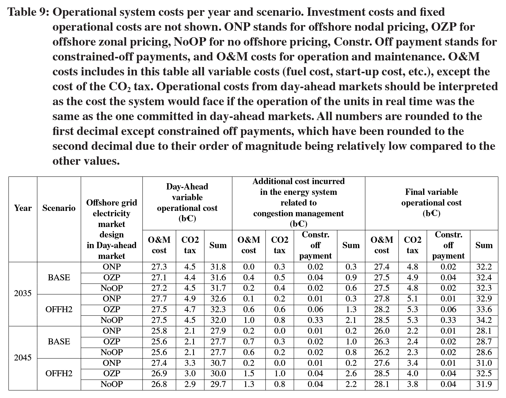
In day-ahead markets, the ONP market design configuration is always the most expensive one though, which is an expected result since it is the most constrained scenario.⁵ In scenario BASE, both OZP and NoOP market designs lead to similar day-ahead operational costs (slightly cheaper for OZP) in 2035 and 2045. In scenario OFFH2, the cheapest offshore market design in day-ahead markets is NoOP for 2035 and 2045. These results suggest that hub-to-shore interconnectors might have higher relative importance than hub-to-hub interconnectors in scenario OFFH2, and similar relative importance in scenario BASE.

The lower costs in day-ahead markets for OZP and NoOP with respect to ONP market design are a result of having ignored part of the transmission constraints. However, after performing the required congestion management both OZP and NoOP configurations end up resulting in a higher final variable energy system cost for both scenarios compared to the ONP configuration (Table 9). These higher final variable energy system costs when using OZP and NoOP configurations compared to the ONP one are linked to higher final operational cost and CO₂ tax (and hence, emissions), which are linked to higher final thermal unit generation, specially from natural gas. The difference in final CO₂ emissions in the studied energy sector varies between 0.6–5.6 Mton/ year depending on the scenario compared to ONP market design. These results highlight that the ONP market design is likely to be the best market configuration in order to fulfill the climate goals. Constrained-off payments tend to play a minor role in final variable system costs. However, this is not the case when using NoOP design in scenario OFFH2 in the year 2035, where these payments correspond to 16% of the cost linked to congestion management. In this scenario 82% of the payments are used to compensate hub-connected wind turbines, which is in line with the high increase of hub-connected offshore wind curtailment after congestion management with respect to day-ahead markets (Table 10). These results suggest that in this case domestic hub-connected lines are highly binding, i.e. they are highly congested in many hours of the year.

Table 10:

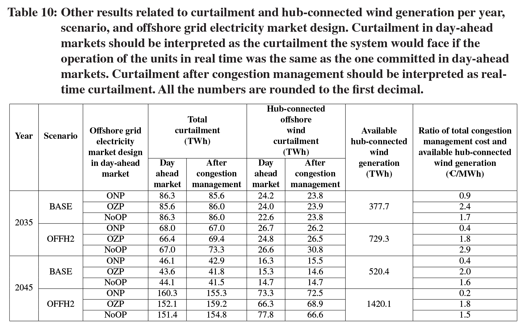
Other results related to curtailment and hub-connected wind generation per year, scenario, and offshore grid electricity market design. Curtailment in day-ahead markets should be interpreted as the curtailment the system would face if the operation of the units in real time was the same as the one committed in day-ahead markets. Curtailment after congestion management should be interpreted as realtime curtailment. All the numbers are rounded to the first decimal.

Year	Scenario	Offshore grid electricity market design in day-ahead market	Total curtailment (TWh)		Hub-connected offshore wind curtailment (TWh)		Available hub-connected wind generation (TWh)	Ratio of total congestion management cost and available hub-connected wind generation (=C/MWh)
Year	Scenario	Offshore grid electricity market design in day-ahead market	Day ahead market	After congestion management	Day ahead market	After congestion management	Available hub-connected wind generation (TWh)
2035	BASE	ONP	86.3	85.6	24.2	23.8	377.7	0.9
		OZP	85.6	86.0	24.0	23.9		2.4
		NoOP	86.3	86.0	22.6	23.8		1.7
	OFFH2	ONP	68.0	67.0	26.7	26.2	729.3	0.4
		OZP	66.4	69.4	24.8	26.5		1.8
		NoOP	67.0	73.3	26.6	30.8		2.9
2045	BASE	ONP	46.1	42.9	16.3	15.5	520.4	0.4
		OZP	43.6	41.8	15.3	14.6		2.0
		NoOP	44.1	41.5	14.7	14.7		1.6
	OFFH2	ONP	160.3	155.3	73.3	72.5	1420.1	0.2
		OZP	152.1	159.2	66.3	68.9		1.8
		NoOP	151.4	154.8	77.8	66.6		1.5

In terms of final variable operational costs, the worst market design for the BASE scenario is OZP for all studied years, although for the scenario OFFH2, the worst one is NoOP in 2035, and OZP in 2045 (Table 9). The ratio of total hub-to-shore electricity transmission capacity and total hub-connected wind generation (Table 4) could be behind the shift in worst market design in scenario OFFH2. In this scenario, this ratio is 0.6 by 2035 and 0.9 by 2045. The lower the number, the higher the importance of the non-captured congestion between the offshore grid and the onshore system when using market design NoOP. The difference in final variable operational costs of alternative market designs and the ONP design ranges from 0.2–1.6 b€/year in the investigated scenarios and years. The difference between market design OZP and ONP increases towards 2050 in both capacity development scenarios, whereas the difference between market design NoOP and ONP increases towards 2050 in scenario BASE, and decreases in scenario OFFH2. These results suggest that the energy system development, and the flexibility in it (partly linked to sector coupling), is likely to influence considerably the impact of the market design on the system operational costs.

The congestion management costs are in absolute numbers higher in the scenario OFFH2 than in the BASE scenario for both OZP and ONP configuration because the offshore grid and wind power development taking place in the OFFH2 scenario are larger (Table 4). The congestion management costs vary between 0.6–1.0 b€/year when not using a ONP market design in the BASE scenario, and between 1.3–2.6 b€/year in the OFFH2 scenario. In terms of share of final variable operational costs, when not using a ONP market design the congestion management costs varies between 2–4% in scenario BASE, and 4–8% in scenario OFFH2. In scenario BASE, congestion management costs are highest when using the OZP configuration in 2035 and 2045, whereas in scenario OFFH2, these costs are highest when using the NoOP configuration in 2035, and the OZP configuration in 2045. For both scenarios, the absolute difference in congestion management cost between the OZP and NoOP market designs decreases towards 2050. This absolute difference reduction towards 2050 could be linked to the system being more flexible by 2045 than by 2035. Congestion management costs are highly influenced by how congested the ignored transmission lines are in real time and the cost of the units used to balance the system. These costs are also related to the loss of congestion rent in day-ahead markets when using alternative market design to ONP (Table 7): high loss of congestion rent generally leads to high congestion management costs.

When calculating the ratio between congestion management cost and the total available hub-connected wind generation (Table 10), the results show relatively similar order of magnitude for both scenarios when not using ONP configuration: 1.6–2.4 €/MWh in the BASE scenario, and 1.5–2.9 €/MWh in the OFFH2 scenario if a ONP market design is not used. This means that the offshore wind generation volumes do not have a significant influence on the congestion management cost per MWh of hub-connected offshore wind available in the studied scenarios. This result could be linked to the approach used to optimise investments in transmission lines, which leads to relatively optimistic and adequate transmission deployment in the system.

The curtailment after congestion management has taken place (Table 10), i.e. curtailment in real time, is also highly dependent on the scenario, market design, and year. These results are highly influenced by the constrained-off payment of the different VRE technologies when using different market designs (which is linked to day-ahead prices), and the congestion of the lines after congestion management is applied. For instance, if in a particular hour day-ahead prices seen in the hubs are high, the penalty for constraining-off the generation of hub-connected wind generators will also be high, and therefore, from a cost-minimisation perspective, curtailment after congestion management is likely to take place only if there is line congestion. It is particularly interesting the case of scenario OFFH2 in year 2045 when using NoOP configuration, which led in day-ahead markets to higher hub-connected offshore wind curtailment compared to ONP configuration, but to a considerable reduction in curtailment after congestion management. These results suggest that the ignored transmission lines in day-ahead markets were highly binding in this case.

Overall, the results obtained are likely to be linked to the magnitude and overall use of the ignored hub-to-hub and hub-to-shore electricity transmission lines in the day-ahead market in the different scenarios, as well as the overall composition of the energy system and the flexibility in it (partly linked to sector coupling). However, it is not straight forward to derive which factor is the main responsible for the results obtained due to the high complexity of the overall studied energy system.

For example, by 2045 in the BASE scenario, when using the OZP configuration for dayahead markets, 10.5 GW (10% of the total hub-connected electricity transmission) are not considered in the day-ahead optimisations to limit transmission flows and lead to a congestion management cost of 1.0 b€, whereas when using the NoOP configuration 5+36.7=41.7 GW (35% of the total hub-connected electricity transmission) are not considered in the day-ahead optimisations to limit transmission flows and lead to an additional cost of 0.8 b€. Therefore, in scenario BASE despite ignoring a larger share of the hub-connected installed capacity when using the NoOP market design in day-ahead markets, the congestion management cost is lower than when using a OZP configuration.

The same analysis done by 2045 for the OFFH2 scenario leads to, when using OZP configuration, ignoring 36.9 GW in day-ahead markets (13% of the total hub-connected electricity transmission capacity) and an additional cost of 2.6 b€, and when using NoOP configuration, to ignoring in day-ahead markets 8.9+161.7=170.6 GW (53% of the total hub-connected electricity capacity) and to a congestion management cost of 2.2 b€. Again, despite ignoring in day-ahead markets a larger share of the hub-connected installed capacity when using the NoOP market design in day-ahead markets, the congestion management cost is lower than when using a OZP configuration.

These results suggest that total ignored offshore transmission line capacity is not the only factor affecting congestion management costs, and therefore, when designing offshore markets, it is likely to be key to identify critical offshore hub-connected transmission lines, i.e. lines that due to the configuration of the integrated energy system are likely to experience high congestion, so they are accounted for in day-ahead markets.

Overall, these results highlight that the impact of the offshore grid market design is highly influenced by the overall configuration of the offshore grid, as well as the rest of the energy system.

3.2.3 Critical reflection

The assumptions of economic rationality and perfect markets are some of the main limitations of the model. Considering that in reality heat markets, electricity markets, and gas market take place with different time schedules during the day could have affected the results of this paper.

In this paper, we have focused on the impact of market design on the operation of the energy system. The modelling of investments has assumed offshore nodal pricing (ONP) for the sake of comparability between scenarios. In reality, a number of factors will determine investment decisions in transmission lines, including the specific market design. Using different energy systems for each offshore electricity market design would have rendered the comparability of scenarios impossible and could hence not be implemented in this paper with the chosen subject of investigation. It is generally expected that, realistically, transmission grids are expanded less than what is deemed optimal in energy system model results. In effect, we may experience very different actual transmission grid expansion, than depicted here. This is something worth investigating in future research.

This paper has used a single weather year in the scenarios. Considering the uncertainties related to the variation of wind generation along the years could have influenced the design of offshore grids, and hence, the impact of the results of this paper. Future research should take this into account.

The uncertainties related to VRE generation in day-ahead markets have not been considered in this paper. Not considering potential forecast errors could have underestimated the impact of the offshore grid electricity market design. This could be of special important when VRE technologies provide most of the electricity of the system. This aspect should also be considered in future research.

The use of the different storage technologies included in the model for congestion management purposes has not been considered in this paper. Strategic bidding in different markets could potentially reduce congestion management costs, at the expense of increasing costs in day-ahead markets. This could be analysed in future research.

The role that sector coupling has played in providing flexibility to reduce congestion management costs has not been analysed in the paper due to space limitations. Most likely, without flexible electricity load, the congestion management costs of the system would have been higher. This is a topic worth investigating in future research.

The reinforcement of distribution grids has not been considered in this study. Considering the large increase of electricity demand towards 2050 that is part of the scenarios of this paper, it is likely that there will be need for such reinforcement. Without reinforcing distribution grids, it is likely that there will be more wind curtailment, as suggested by Tosatto et al. (2021).

The simplified approach to model energy flows used in the paper, which is based on linear flows using net transfer capacity, is done for the sake of computational complexity. It could have led to too optimistic trading volumes, and hence, underestimated the costs of the energy system. More advanced modelling of electricity, H₂, and/or heat flows could further improve the results of the model.

Due to modelling limitations the congestion management cost is not 0 in the ONP configuration even though the energy system considered is exactly the same (Table 9). This limitation is related to using a limited foresight of one hour in the congestion management optimisations and allowing to start up and shut down fast units. The weight of start-up/shut-down/online costs in the objective function with respect to other operational costs is different in day-ahead optimisations (where the foresight is 24 hours) to congestion management optimisations (where the foresight is 1 hour). Nevertheless, this difference is relatively small in all scenarios (less than 0.3 b€/year (Table 9)), and therefore, we believe the conclusions from this paper are robust.

Finally, in this study we assume perfect competition for all market design runs and ignore possible market power execution (discussed in Section 1.1) and strategic bidding of generators that can lead to additional costs for the energy system. And these costs at the end can also vary between different zonal configurations and market designs. However, as the scope of this paper is to derive findings related to a well-regulated market and optimal design, we neglect market power issues and can still hold our main conclusions related to a theoretically and practically optimal market configuration for offshore energy hubs.

4. Conclusions

This paper has investigated the impact of different electricity market offshore designs on the operation of day-ahead markets, as well as the impact on the required congestion management on integrated energy systems towards 2050. We have done this through an advanced optimisation process using the open-source energy system model Balmorel.

Our analysis confirms the well-known concept of nodal pricing as cost-effective market configuration. We show for an advanced and integrated offshore electricity market that offshore nodal pricing (ONP), where each offshore hub represents its own bidding zone, minimises costs (0.2–1.6 b€/year lower) and CO₂ emissions (0.6–5.6 Mton/year lower) compared to the two alternatives, i.e. where all hubs form a unique offshore bidding zone (OZP) or no offshore bidding zone is introduced at all (NoOP). Specifically, alternative designs to offshore nodal pricing lead to 0.5–2% higher final variable operational costs in a scenario with limited offshore H₂ generation (BASE) and 2.1–5% higher cost in a scenario with substantial offshore H₂ generation (OFFH2).

Price results and congestion rents are highly dependent on the offshore grid and market configuration, and differ between the investigated years. The impact is not uniform across countries. Offshore wind generation volumes are not found to have a significant influence on the congestion management cost per MWh of hub-connected offshore wind.

The impact of different market designs is highly dependent on the overall configuration of the offshore grid, as well as the availability of H₂ generation. Higher flexibility in offshore grids and in the rest of the system might reduce the spread between the designs and thus help mitigate implications of suboptimisation.

Our results confirm that nodal pricing in offshore grids is preferable over price zones or no offshore pricing at all. Choosing this market configuration can thus contribute to pave the way for a cost-effective energy transition to carbon neutrality in Europe in 2050.

Supplemental Material

sj-pdf-1-enj-10.5547_01956574.45.4.jgea – Supplemental material for Offshore Market Design in Integrated Energy systems: A Case Study on the North Sea Region towards 2050

Supplemental material, sj-pdf-1-enj-10.5547_01956574.45.4.jgea for Offshore Market Design in Integrated Energy systems: A Case Study on the North Sea Region towards 2050 by Juan Gea-Bermúdez, Lena Kitzing and Dogan Keles in The Energy Journal

Footnotes

Acknowledgements

The authors would like to acknowledge Maksym Pavlyuk’s data support for this paper.

1.

The branch used for the data and code used in this paper is called “H2_Transport_update_2021_JGB” (last access 1st September 2021)

2.

The energy system capacity development scenario for the OFFH2 scenario presented corresponds to the LP run. This is because the MIP run optimisation did not manage to converge in less than two weeks due to its high complexity. The influence of not using the MIP run on the overall results is likely to be very small. In the BASE scenario, the system cost difference between the MIP and LP run is lower than 0.091% in each of the studied years.

3.

The CO₂ emissions corresponding to the transport sector that is not part of the model, i.e. the use of traditional fossil fuels for transport, are derived based on [European Environment Agency, 2020]. Additional GHG emissions that are part of the energy sectors covered by the model are estimated assuming that the CO₂ emissions are 96.85% of the total GHG emissions of the studied system using data from [European Environment Agency, 2020]

4.

Since there is no offshore grid development in 2025 in the scenarios, the impact of the market design has been run only for the years 2035 and 2045.

5.

Results from day-ahead markets should be interpreted as the costs, generation, curtailment, etc., the system would face if the operation of the units in real time was the same as the one committed in day-ahead markets

References

Balmorel community (2021a). Balmorel code. https://github.com/balmorelcommunity/Balmorel.

Balmorel community (2021b). Balmorel data. https://github.com/balmorelcommunity/Balmorel_data.

Bertsch

Brown

Hagspiel

Just

(2017). “The relevance of grid expansion under zonal markets.” The Energy Journal 38(5). https://doi.org/10.5547/01956574.38.5.jber.

Bramstoft

Alonso

Jensen

Ravn

Munster

(2020). “Modelling of Renewable Gas And Fuels In Future Integrated Energy Systems.” Applied Energy 268. https://doi.org/10.1016/j.apenergy.2020.114869.

Bundesnetzagentur (2021). Bericht netzengpassmanagement-gesamtes jahr 2021. https://www.bundesnetzagentur.de/SharedDocs/Downloads/DE/Sachgebiete/Energie.

Commission

Centre

J.R.

Antonopoulos

Vitiello

Fulli

Masera

(2020). Nodal pricing in the European internal electricity market. Publications Office.

Danish Energy Agency (2021). Technology Catalogues.

DW (2021). Denmark to construct artificial island as a wind energy hub.

EA Energy Analysis (2020). Offshore wind and infrastructure.

10.

EDMOnet-Bathymetry (2021). EMODnet DTM.

11.

European Commission (2018). A Clean Planet for all A European long-term strategic vision for a prosperous, modern, competitive and climate neutral economy.

12.

European Environmental Agency (2020). EEA greenhouse gas-data viewer.

13.

Flex4RES project (2019). Flexible Nordic Energy Systems summary report.

14.

Frank

A. Wolak

(1999). Report of Redesign of California Real-Time Energy and Ancillary Services Markets.

15.

Gea-Bermúdez

(2021). “Optimizing the future North Sea integrated energy system.” PhD thesis.

16.

Gea-Bermúdez

Bramstoft

Koivisto

Kitzing

Ramos

(2023). “Going offshore or not: Where to generate hydrogen in future integrated energy systems?” Energy Policy 174: 113382. https://doi.org/10.1016/j.enpol.2022.113382.

17.

Gea-Bermúdez

Das

Koivisto

M.J.

koduvere

(2021). “Day-ahead Market Modelling of Large- scale Highly-renewable Multi-energy Systems: Analysis of the North Sea Region Towards 2050.” Energies 14. https://doi.org/10.3390/en14010088.

18.

Gea-Bermúdez

Jensen

I.G.

Münster

Koivisto

Kirkerud

J. G.

kuang Chen

Ravn

(2021). “The role of sector coupling in the green transition: A least-cost energy system development in northern-central Europe towards 2050.” Applied Energy 289, 116685. https://doi.org/10.1016/j.apenergy.2021.116685.

19.

Gea-Bermúdez

Kitzing

Koivisto

Das

Murcia

J.P.

León Sørensen

(2022). “The value of sector coupling for the development of offshore power grids.” Energies 15(3). https://doi.org/10.3390/en15030747.

20.

Gea-Bermúdez

Pade

L.L.

Koivisto

M.J.

Ravn

(2020). “Optimal generation and transmission de- velopment of the north sea region: Impact of grid architecture and planning horizon.” Energy 191: 116512. https://doi.org/10.1016/j.energy.2019.116512.

21.

Gunkel

P.A.

Bergaentzlé

Græsted Jensen

Scheller

(2020). “From passive to active: Flexibility from electric vehicles in the context of transmission system development.” Applied Energy 277: 115526. https://doi.org/10.1016/j.apenergy.2020.115526.

22.

Gunkel

P.A.

Koduvere

Kirkerud

J.G.

Fausto

F.J.

Ravn

(2020). “Modelling transmission systems in energy system analysis: A comparative study.” Journal of Environmental Management 262: 110289. https://doi.org/10.1016/j.jenvman.2020.110289.

23.

Harvey

S.M.

Hogan

W.W.

(2000). “Nodal and zonal congestion management and the exercise of market power. Henney, A. (1998). Contrasts in restructuring wholesale electric markets: England/Wales, California, and the pjm. The Electricity Journal 11(7): 24–42. https://doi.org/10.1016/S1040-6190(98)00074-8.

24.

Henning

H.-M.

Palzer

(2014). “A comprehensive model for the german electricity and heat sector in a future energy system with a dominant contribution from renewable energy technologies—part i: Methodology.” Renewable and Sustainable Energy Reviews 30: 1003–1018. https://doi.org/10.1016/j.rser.2013.09.012.

25.

Holmberg

Lazarczyk

(2015). “Comparison of congestion management techniques: Nodal, zonal and discriminatory pricing.” The Energy Journal 36(2). https://doi.org/10.5547/01956574.36.2.7.

26.

IPCC (2022). Contribution of Working Group II to the Sixth Assessment Report of the Intergovernmental Panel on Climate Change [ Pörtner

H.-O.

Roberts

D.C.

Tignor

Poloczanska

E.S.

Mintenbeck

Alegría

Craig

Langsdorf

Löschke

Möller

Okem

Rama

(eds.)]. Cambridge University Press. In Press. Intergovernmental panel on climate change. https://www.ipcc.ch/report/ar6/wg2/downloads/report.

27.

IRENA (2019). Renewable Power Generation Costs in 2018.

28.

Jansen

Duffy

Green

T.C.

Staffell

(2022). “Island in the sea: The prospects and impacts of an offshore wind power hub in the north sea.” Advances in Applied Energy 6: 100090. https://doi.org/10.1016/j.adapen.2022.100090.

29.

Jensen

I.G.

Wiese

Bramstoft

Münster

(2020). “Potential role of renewable gas in the transition of electricity and district heating systems.” Energy Strategy Reviews 27(November 2019): 100446. https://doi.org/10.1016/j.esr.2019.100446.

30.

Koivisto

Das

Guo

Sørensen

Nuño

Cutululis

Maule

(2019). “Using time series simulation tools for assessing the effects of variable renewable energy generation on power and energy systems.” Wiley Interdisciplinary Reviews: Energy and Environment 8(3): e329. https://doi.org/10.1002/wene.329.

31.

Koivisto

Gea-Bermúdez

Sørensen

. (2019, November). “North sea offshore grid development: Combined optimization of grid and generation investments towards 2050.” IET Renewable Power Generation. https://doi.org/10.1049/iet-rpg.2019.0693.

32.

Konstantelos

Pudjianto

Strbac

De Decker

Joseph

Flament

Kreutzkamp

Genoese

Rehfeldt

Wallasch

A.-K.

Gerdes

Jafar

Yang

Tidemand

Jansen

Nieuwenhout

van der Welle

Veum

(2017). “Integrated north sea grids: The costs, the benefits and their distribution between countries.” Energy Policy 101: 28–41. https://doi.org/10.1016/j.enpol.2016.11.024.

33.

Kunz

. (2013, October). “Improving congestion management: How to facilitate the integration of renewable generation in Germany.” The Energy Journal 34(4). https://doi.org/10.5547/01956574.34.4.4.

34.

Lester

M.S.

Bramstoft

Münster

(2020). “Analysis on Electrofuels in Future Energy Systems: A 2050 Case Study.” Energy 199: 117408. https://doi.org/10.1016/j.energy.2020.117408.

35.

Münster

Morthorst

P.E.

Larsen

H.V.

Bregnbæk

Werling

Lindboe

H.H.

Ravn

. (2012). “The role of district heating in the future Danish energy system.” Energy 48(1): 47–55. 6th Dubrovnik Conference on Sustainable Development of Energy Water and Environmental Systems, SDEWES 2011. https://doi.org/10.1016/j.energy.2012.06.011.

36.

Newbery

D.M.

(2018). “What future(s) for liberalized electricity markets: efficient, equitable or innovative?” The Energy Journal 39(1). https://doi.org/10.5547/01956574.39.1.dnew.

37.

Nordic Energy Research and International Energy Agency (2016). Nordic Energy Technology Perspectives 2016 report.

38.

North Sea Power Hub (2020). North Sea wind power hub programme.

39.

Nuño

Maule

Hahmann

Cutululis

Sørensen

Karagali

(2018). “Simulation of transcontinental wind and solar PV generation time series.” Renewable Energy 118: 425–436. https://doi.org/10.1016/j.renene.2017.11.039.

40.

Philip Swisher (2020). “Modelling of Political and Technological Innovation on Northern Europe’s Energy System Towards 2050.”

41.

Poncelet

Delarue

D’haeseleer

(2020). “Unit commitment constraints in long-term planning models: Relevance, pitfalls and the role of assumptions on flexibility.” Applied Energy 258: 113843. https://doi.org/10.1016/j.apenergy.2019.113843.

42.

Rehfeldt

Fleiter

Toro

(2018). “A bottom-up estimation of the heating and cooling demand in European industry.” Energy Efficiency 11: 1057–1082. https://doi.org/10.1007/s12053-017-9571-y.

43.

Ruiz

Nijs

Tarvydas

Sgobbi

Zucker

Pilli

Jonsson

Camia

Thiel

Hoyer-Klick

Longa

F. D.

Kober

Badger

Volker

Elbersen

Brosowski

Thrän

(2019). “Enspreso - an open, EU-28 wide, transparent and coherent database of wind, solar and biomass energy potentials.” Energy Strategy Reviews 26: 100379. https://doi.org/10.1016/j.esr.2019.100379.

44.

Sims

R.E.

Mabee

Saddler

J.N.

Taylor

(2010). “An overview of second generation biofuel technologies.” Bioresource Technology 101(6): 1570–1580. https://doi.org/10.1016/j.biortech.2009.11.046.

45.

The European Commission (2020a). Climate strategies and targets.

46.

The European Commission (2020b). EU strategy on offshore renewable energy.

47.

Tosatto

Beseler

Østergaard

Pinson

Chatzivasileiadis

(2021). “North Sea energy islands: Impact on national markets and grids.” Energy Policy 167: 112907. https://doi.org/10.1016/j.enpol.2022.112907.

48.

Transport and Environment (2018). How to decarbonize the transport sector by 2050.

49.

Wiese

Baldini

(2018). “Conceptual model of the industry sector in an energy system model: A case study for Denmark.” Journal of Cleaner Production 203: 427–443. https://doi.org/10.1016/j.jclepro.2018.08.229.

50.

Wiese

Bramstoft

Koduvere

Alonso

A.P.

Balyk

Kirkerud

J.G.

Åsa Grytli Tveten Bolkesjø

T.F.

Münster

Ravn

(2018). “Balmorel open source energy system model.” Energy Strategy Reviews 20: 26–34. https://doi.org/10.1016/j.esr.2018.01.003.

Supplementary Material

Please find the following supplemental material available below.

For Open Access articles published under a Creative Commons License, all supplemental material carries the same license as the article it is associated with.

For non-Open Access articles published, all supplemental material carries a non-exclusive license, and permission requests for re-use of supplemental material or any part of supplemental material shall be sent directly to the copyright owner as specified in the copyright notice associated with the article.

0.00 MB

1.18 MB