Export Diversification and Energy Consumption Efficiency in the Light of Non-linear Evidence

Abstract

We estimate the effects of export dynamics on energy consumption using a balanced panel of 95 economies and three subsamples, i.e., low- and lower-middle-income (LMEs), upper-middle-income (UMEs), and high-income (HIEs) from 1997 to 2013. We show the non-linear linkages between export diversification (ED) and energy use. More specifically, we show the inverted-U shape ED effects on energy use per output unit. This result implies the increases in energy inefficiency in the progress of diversification improvement in exports until a threshold level from which ED would help to enhance energy efficiency. Our analysis of the three subsamples shows consistent findings regarding the effects of ED across income levels. The inverted-U shape effects of ED are consistent in LMEs and UMEs, while it is ambiguous in HIEs. The results suggest that low and middle economies should diversify exports as much as possible to pass the threshold, where diversification can improve energy efficiency.

Keywords

Exports Diversification Energy consumption Energy efficiency Panel data

1. Introduction

Against the backdrop of climate change and global warming, reducing energy consumption is one of the most urgent policy actions (UN, 2020). One feasible option to support this process is to improve energy efficiency, which enhances energy security and economic growth (Le & Nguyen, 2019). Several studies (Nguyen et al., 2018; Phuc Nguyen et al., 2019; Tiba & Frikha, 2018) examine the impacts of economic integration, i.e. trade openness, on CO2 emissions or energy consumption. More recently, Bashir et al. (2020) examined the impacts of export product diversification on energy intensity in a sample of 29 OECD countries from 1990—2015. They find that export diversification (ED) can contribute to decreasing energy and carbon intensity. However, there is no current study on the impacts of ED¹ on the efficiency of energy consumption globally. We use energy efficiency instead of intensity in our analysis to better understand the relationship, as efficiency can affect energy intensity, and efficiency improvements in processes and other factors can contribute to changes in energy intensity.² Since most OECD countries are advanced economies with high development status, they are in the stage of high technological development and energy consumption efficiency. In contrast, developing countries may not be in good condition of technologies or economic development (Canh, Schinckus, et al., 2019; Phuc Nguyen et al., 2019) and thus the effect of ED on energy intensity may not be as found in advanced countries. Moreover, recent studies, e.g., Le et al. (2020) and Canh and Dinh Thanh (2020), emphasize that the export diversification process brings both pros and cons with benefits and costs. Therefore, the ED appears to have non-linear effects on economic factors such as income inequality (Le et al., 2020) and shadow economy (Canh & Dinh Thanh, 2020).

1.
The Export Diversification measures the export product diversification (see https://www.imf.org/external/np/res/dfidimfydiversification.htm)

Energy intensity measures the quantity of energy required per unit of output or activity. In contrast, energy efficiency represents the changes in the amounts of energy inputs or services for a given amount of energy input.

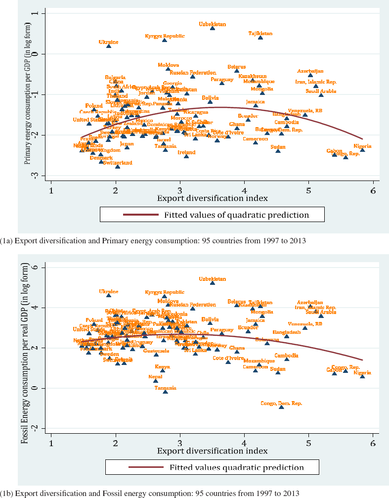
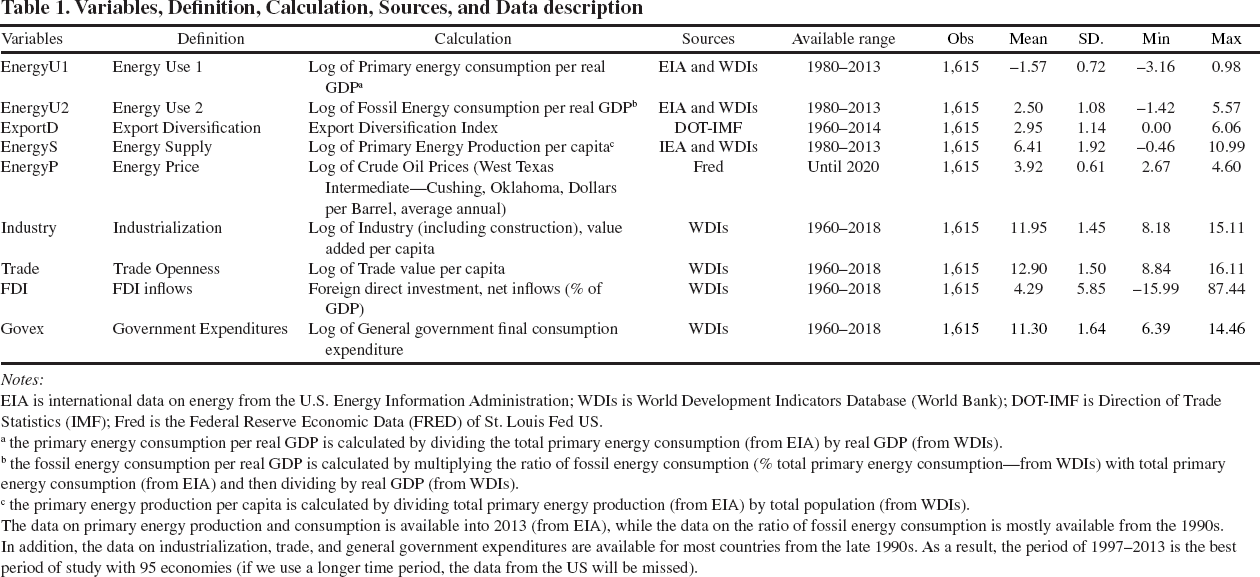
To shed further light on the relationship between export diversification and energy consumption, this paper estimates the effects of export dynamics on energy consumption using a balanced panel of 95 economies and three subsamples, i.e., low- and lower-middle-income (LMEs), upper-middle-income (UMEs), and high income (HIEs) from 1997 to 2013. To motivate our paper, we first present Figure 1, which shows the non-linear (inverted-U shaped) relationships between the export diversification index from IMF and the primary energy consumption per real GDP (Figure la) and fossil energy consumption per real GDP (Figure lb). As defined by the IMF, higher values for the ED index indicate lower diversification.

There are numerous economic reasons that could lead to a non-linear relationship between ED and energy use. For example, although Shahbaz et al. (2019) show that ED increases energy demand in the long run for the US, Le and Nguyen (2019) show that ED might be both beneficial and costly for domestic economic activities. For example, ED might benefit employment (Egger & Etzel, 2012), productivity (Njikam, 2017), poverty reduction (Le et al., 2020), and economic reform (Schrank, 2005). Thus, increases in ED may result in line with investment in technological advancement (Xuefeng & Yaşar, 2016), which enhances energy efficiency as the structural changes in production technology. However, ED is also linked with high initial costs for new production or new market entry (Aw & Lee, 2017; Hoffman et al., 2016), resulting in low technology investment for cost savings. This high cost of the diversification process may lead to the wisdom of "growth first, clean later," as proposed in the Environmental Kuznets Curve hypothesis (EKC). As a result, ED could lead to higher energy inefficiency and, hence, lower energy demand. Consequently, the (non)-linear empirical effects of ED (as measured by the ED index) on energy efficiency depend on various factors one utilizes to analyse the research objectives.

This study differs from previous studies (e.g. Shahbaz et al. (2019) while contributing to the current study on the impacts of ED on energy intensity (see Bashir et al. (2020) by extending the impacts of ED on the efficiency of energy consumption in a global sample. Moreover, we use a global sample and three subsamples, including low- and lower-middle-income (LMEs), upper-middle-income (UMEs), and high-income (HIEs), which broadens the literature on global evidence. The paper adapts a recent study by Canh et al. (2020) in calculating two proxies of energy efficiency, i.e., the efficiency of energy use in production and energy efficiency use in consumption, separately. Notably, we base our empirical approach on a new line of literature on the impacts of ED on economic factors (e.g., Le et al. (2020) and Canh and Dinh Thanh (2020)) to investigate the non-linear impacts of ED on the efficiency of energy use. Empirically, we estimate ED's effects on primary energy use per output unit and fossil energy use per output unit. We control for the effects of energy supply, energy prices, and other factors such as industrialization, FDI inflows, government expenditures, and trade openness. We use 97 countries from 1997 to 2013 as an empirical sample. Due to the availability of energy consumption data, our sample ended in 2013³. The panel-corrected standard errors (PCSE) model is applied as the primary estimator to deal with cross-sectional dependence. Moreover, we use the feasible general least squares (FGLS) and two-step GMM models as robustness checks to address heteroscedasticity and endogeneity issues.

This is best period of data from the World Development Indicators database of World Bank (version 2020).

Figure 1

Export Diversification and Energy use: 95 countries from 1997 to 2013

Our main empirical results are as follows. We first document that there are mutual causalities between ED and both variables of energy use. Second, our panel estimation shows the in-verted-U shape effects of ED on energy use per output unit and fossil energy use per output unit, respectively. Consequently, our results indicate that the increases in export diversification may lead to higher energy use (or lower energy efficiency) until a threshold level, from which the increases in export features would enhance the energy efficiency. Third, the estimations for three subsam-ples show consistent inverted-U shape impacts of ED on energy use in LMEs and UMEs, which is unclear in HIEs. The results have two important implications. Firstly, the export diversification strategy should be supported by governments, especially in LMEs and UMEs, as much as possible to overcome the threshold to improve energy efficiency. Secondly, the diversification of exports at the initial stage is one of the causes of environmental degradation due to higher energy consumption: It must be backed by suitable policies for firms to transform their production technology as soon as possible.

The paper is structured as follows. The next section is the literature review. In Section 3, we discussed methodology and data. Results are presented and discussed in Section 4. The final section 5 comes with the conclusion.

2. Literature Review

The urgency in reducing energy intensity (Sadorsky, 2013) and raising energy consumption efficiency (Bye et al., 2018) are paid more attention to in the literature on energy—and environmental economics than in sustainable development. That is, the understanding of energy use's drivers is paid more attention to energy and environmental economics (Adom & Adams, 2018; Bye et al., 2018; Chen & Lei, 2018). The IPAT model (the Influence, Population, Affluence, and Technology) is first proposed by Ehrlich and Holdren (1971), and then the STIRPAT model (the Stochastic Impacts by Regression on Population, Affluence, and Technology) by Dietz and Rosa (1997), as an extension of IPAT, who have linked the human activities, especially economic activities to environmental degradation. In this line of literature, the impacts of economic activities on energy consumption, which cause CO2 emissions and then global warming and climate change, are paid huge interest, but the conclusions are still mixed (Chen, 2018; Hanif, 2018; Saidi et al., 2017). On the other hand, the Environmental Kuznets Curve hypothesis (EKC) indicates that the relationship between economic development and environmental quality is an inverted-U shape (Rashid Gill et al., 2018; Sun, 1999). The EKC theory explains that energy consumption, such as coal, fuel, and gas, is increased much more in the economic development process of poor economies by the wisdom of "grow first, clean up later" (Rock & Angel, 2007). Environment quality is paid more attention in high-income economies when the country attains a certain threshold of economic development, from which the citizens demand regulatory institutions and actions to protect the environment (Azadi et al., 2011). In addition to the STIRPAT model or EKC hypothesis, other factors, i.e., urbanization (Kasman & Duman, 2015; Zang et al., 2017), industrialization (Jiang & Lin, 2012), economic integration (Phuc Nguyen et al., 2019), shadow economy (Canh, Thanh, et al., 2019) are suggested as drivers of CO2 emissions or energy consumption in general. Recently, Shahbaz et al. (2019) showed that export diversification is linked with higher energy demand in the long run in the case of the US over the period 1975-2016. The features of export activities, i.e., export diversification and export quality, have been an interesting topic in recent years from both international organizations such as the IMF and research attention (Osakwe et al., 2018).

On the one hand, ED positively affects domestic economic diversification (Albassam, 2015), which is linked with new economic activities through entrepreneurship (Schrank, 2005). Contractor and Kundu (2004) indicate that export-led strategies are better at stimulating economic growth than inward-looking ones. ED is also argued as a positive factor in employment (Egger & Etzel, 2012), domestic firm productivity (Njikam, 2017), and economic reform (Schrank, 2005). A higher ED may lead to more economic activities, which might be invested in technological advancement (Xuefeng & Yaşar, 2016). As a result, ED may lead to higher energy efficiency due to structural changes in production. However, ED also has its cons. The literature shows that diversification to a new market or new products is faced with high initial entry costs (Aw & Lee, 2017; Hoffman et al., 2016).

For instance, Fillat et al. (2015) notice that multinational activities come with diversification benefits and fixed—and sunk costs of entry into new markets or products. These costs are primarily exogenous and vary across markets and products; thus, the export-diversification strategy may face more vulnerability. In this vein, Vannoorenberghe et al. (2016) document higher volatility faced by small Chinese firms in expanding the scope of their export partners. Xuefeng and Yaşar (2016) show that a higher cost in the initial stage of export diversification is due to firms' lack of knowledge and experience. Furthermore, ED is also linked with higher international competition from international producers and systematic international risk (Jones et al., 2011). Jones et al. (2011) argue that higher export diversification would imply more significant exposures toward systematic international risks, which could pose local economic agencies in a more challenging and riskier ecosystem by investing in economic activities in low technology to save costs. In the constraints of initial costs and international risk exposures, the new economic activities or the economic transformation of domestic firms may follow the wisdom of "growth first, clean later" as proposed in the Environmental Kuznets Curve hypothesis (EKC).

In contrast, economic activities are executed in high energy inefficiency following export diversification, especially in the initial process. In summary, ED can be hypothesized to cause higher energy use until a threshold, which helps reduce energy use as the higher benefits of ED through the scale of economics. There may be an inverted-U shape relationship between ED and energy use. Therefore, we hypothesize that ED has a non-linear impact on energy use. Furthermore, the increases in ED at the initial stage are linked with high initial costs of entry and competition, while economic agents may follow the EKC hypothesis; thus, they would expand economic activities into high energy-intensive sectors. Therefore, an additional hypothesis can be formed as ED has inverted-U impacts on energy use.

There are already some studies on the non-linear relationship between ED and economic factors, i.e., firm productivity (Xuefeng & Yaşar, 2016) and income inequality (Le & Nguyen, 2019). Nevertheless, there is no study on the non-linear impacts of ED on energy use. The following section presents the methodology and data to investigate the impacts of ED on energy use.

3. Methodology and Data

In this study, we investigate the non-linear impacts of ED (ExportD) on energy use (Energy U) on energy use with a focus on energy efficiency in producing an output unit by building the function of energy use as follows. First, the energy consumption function has two main control variables: energy supply (EnergyS) (Azam et al., 2015) and energy price (EnergyP) (Omri & Nguyen, 2014). In fact, supply and price are two common drivers of any consumption function of any product.

Our explanatory variables differ from the Stochastic Impacts by Regression on Population, Affluence, and Technology (STIRPAT) model that has been often used in the environmental economics literature. Since our analysis focuses on the energy efficiency in production (energy use per output unit), unlike the STIRPAT, we find that industrialization would be more critical (Lin & Zhu, 2017) than urbanization. Moreover, we normalize our variables per capita, and hence, we also do not include the total population as one of our variables. However, we include Trade openness (Trade), FDI inflows (FDI), and government expenditures (Govex) as control variables for sensitivity check the proxies of economic integration and government role (Phuc Nguyen et al., 2019). More importantly, we include ED and the squared term of ED to examine the non-linear impacts of ED on energy use. The empirical investigation of energy intensity is formed by panel estimation of country level:

\begin{matrix} E n e r g y U_{i t} = & α_{0} + α_{1} E x p o r t D_{i t} + α_{2} E x p o r t D_{i t}^{2} + β_{1} E n e r g y_{i t} + β_{2} E n e r g y_{i t} + β_{3} I n d u s t r y_{i t} \\ + β_{4} T r a d e_{i t} + β_{5} F D I_{i t} + β_{6} G o v e x_{i t} + γ_{i} + \partial_{t} + ε_{i t} \end{matrix}

in which: i, t denote for country i at year t. α and β are estimated coefficients. γ_i and ∂ are country and year effects, respectively; ∊_it is residual terms.

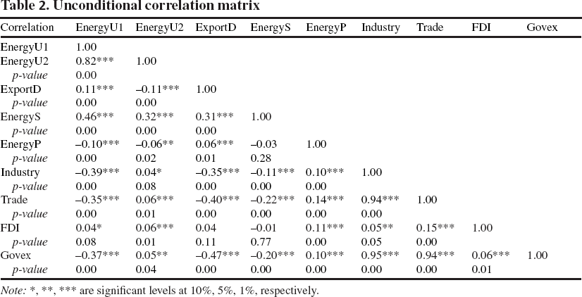
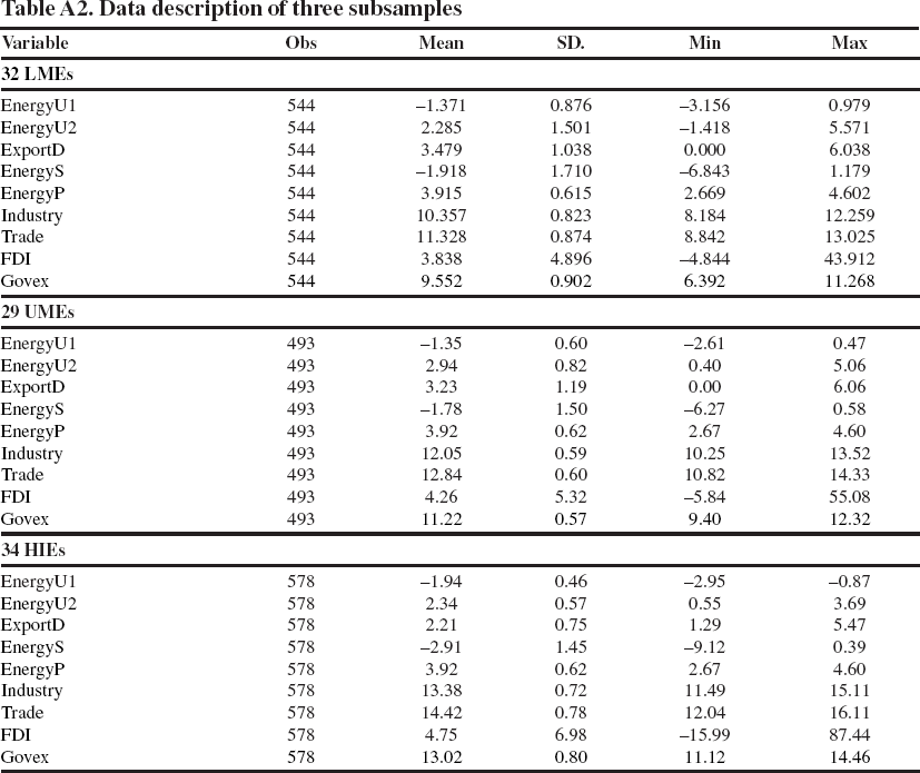
In terms of data, the primary energy consumption and production are collected from the U.S. Energy Information Administration (EIA), which has data until 2013, and most countries have data from the late 1997s. We also collect the fossil energy consumption ratio from World Development Indicators (World Bank) to use as an alternative proxy of energy use besides the primary energy consumption from EIA. The export diversification index is collected from the Direction of Trade Statistics (IMF), which has data until 2014. All remained variables are collected from World Development Indicators (World Bank). The energy use (total primary and fossil energy consumption) is calculated per real GDP. The export diversification is the index from IMF, which is kept as original. The energy supply (primary energy production) is calculated per capita. The industrial value, trade value, and government expenditures are calculated per capita. All variables, excluding the case of export diversification and FDI inflows, are taking in logarithms forms as a standard procedure to normalize data. Due to the availability of data and time constraints of data, the final sample includes 95 countries (see Table Al, Appendix, for list of countries) over the period 1997-2013 (see column 5 in Table 1 for the available time range of each variable). Variables, definitions, detailed calculations, sources, available time range, and data description are presented in Table 1. Moreover, the full sample is divided into three subsamples, including 32 low- and Lower-middle-income economies (LMEs), 24 upper-middle-income economies (UMEs), and 34 high-income economies (HIEs) (see Table A2, Appendix, for the data description of three subsamples). Table 2 reports the unconditional correlation matrix among variables.

Econometrical speaking, our sample has many countries (N=95) but a relatively short time period (1997-2013, i.e. T=17 years). The Pesaran's CD test by Pesaran (2004) is recruited to examine the existence of cross-sectional dependence. The Pesaran (2007)'s CIPS (Z(t-bar)) unit root test and Levin-Lin-Chu unit-root test (Levin et al., 2002) are employed to check the stationarity of variables. Table 3 shows that all variables have cross-sectional dependence, while most are stationary at levels. In this case, the panel-corrected standard errors model (PCSE) estimation is suggested as a suitable estimator for small panel data with short T and large N in the existence of cross-sectional dependence (Bailey & Katz, 2011; Jönsson, 2005; Marques & Fuinhas, 2012), which is recruited as a primary technique in this study.

Table 1
Variables, Definition, Calculation, Sources, and Data description

Variables Definition Calculation Sources Available range Obs Mean SD. Min Max

Energy U1 Energy Use 1 Log of Primary energy consumption per real GDP^a EIAandWDIs 1980-2013 1,615 -1.57 0.72 -3.16 0.98

EnergyU2 Energy Use 2 Log of Fossil Energy consumption per real GDP^b EIA and WDIs 1980-2013 1,615 2.50 1.08 -1.42 5.57

ExportD Export Diversification Export Diversification Index DOT-IMF 1960-2014 1,615 2.95 1.14 0.00 6.06

EnergyS Energy Supply Log of Primary Energy Production per capita^c IEA and WDIs 1980-2013 1,615 6.41 1.92 -0.46 10.99

EnergyP Energy Price Log of Crude Oil Prices (West Texas Intermediate—Cushing, Oklahoma, Dollars per Barrel, average annual) Fred Until 2020 1,615 3.92 0.61 2.67 4.60

Industry Industrialization Log of Industry (including construction), value added per capita WDIs 1960-2018 1,615 11.95 1.45 8.18 15.11

Trade Trade Openness Log of Trade value per capita WDIs 1960-2018 1,615 12.90 1.50 8.84 16.11

FDI FDI inflows Foreign direct investment, net inflows (% of GDP) WDIs 1960-2018 1,615 4.29 5.85 -15.99 87.44

Govex Government Expenditures Log of General government final consumption expenditure WDIs 1960-2018 1,615 11.30 1.64 6.39 14.46

Variables	Definition	Calculation	Sources	Available range	Obs	Mean	SD.	Min	Max
Energy U1	Energy Use 1	Log of Primary energy consumption per real GDP^a	EIAandWDIs	1980-2013	1,615	-1.57	0.72	-3.16	0.98
EnergyU2	Energy Use 2	Log of Fossil Energy consumption per real GDP^b	EIA and WDIs	1980-2013	1,615	2.50	1.08	-1.42	5.57
ExportD	Export Diversification	Export Diversification Index	DOT-IMF	1960-2014	1,615	2.95	1.14	0.00	6.06
EnergyS	Energy Supply	Log of Primary Energy Production per capita^c	IEA and WDIs	1980-2013	1,615	6.41	1.92	-0.46	10.99
EnergyP	Energy Price	Log of Crude Oil Prices (West Texas Intermediate—Cushing, Oklahoma, Dollars per Barrel, average annual)	Fred	Until 2020	1,615	3.92	0.61	2.67	4.60
Industry	Industrialization	Log of Industry (including construction), value added per capita	WDIs	1960-2018	1,615	11.95	1.45	8.18	15.11
Trade	Trade Openness	Log of Trade value per capita	WDIs	1960-2018	1,615	12.90	1.50	8.84	16.11
FDI	FDI inflows	Foreign direct investment, net inflows (% of GDP)	WDIs	1960-2018	1,615	4.29	5.85	-15.99	87.44
Govex	Government Expenditures	Log of General government final consumption expenditure	WDIs	1960-2018	1,615	11.30	1.64	6.39	14.46

Notes:

EIA is international data on energy from the U.S. Energy Information Administration; WDIs is World Development Indicators Database (World Bank); DOT-IMF is Direction of Trade Statistics (IMF); Fred is the Federal Reserve Economic Data (FRED) of St. Louis Fed US.

the primary energy consumption per real GDP is calculated by dividing the total primary energy consumption (from EIA) by real GDP (from WDIs).

the fossil energy consumption per real GDP is calculated by multiplying the ratio of fossil energy consumption (% total primary energy consumption—from WDIs) with total primary energy consumption (from EIA) and then dividing by real GDP (from WDIs).

the primary energy production per capita is calculated by dividing total primary energy production (from EIA) by total population (from WDIs).

The data on primary energy production and consumption is available into 2013 (from EIA), while the data on the ratio of fossil energy consumption is mostly available from the 1990s.

In addition, the data on industrialization, trade, and general government expenditures are available for most countries from the late 1990s. As a result, the period of 1997-2013 is the best period of study with 95 economies (if we use a longer time period, the data from the US will be missed).

Table 2

Unconditional correlation matrix

Correlation	Energy U1	EnergyU2	ExportD	EnergyS	EnergyP	Industry	Trade	FDI	Govex
Energy U1	1.00
EnergyU2	0.82***	1.00
p-value	0.00
ExportD	0. 11***	—0 11***	1.00
p-value	0.00	0.00
EnergyS	0.46***	0. 32***	0.31***	1.00
p-value	0.00	0.00	0.00
EnergyP	-0.10***	-0.06**	0.06***	-0.03	1.00
p-value	0.00	0.02	0.01	0.28
Industry	—0 39***	0.04*	-0.35***	-0.11***	0.10***	1.00
p-value	0.00	0.08	0.00	0.00	0.00
Trade	-0.35***	0.06***	-0.40***	-0.22***	0.14***	0.94***	1.00
p-value	0.00	0.01	0.00	0.00	0.00	0.00
FDI	0.04*	0.06***	0.04	-0.01	0.11***	0.05**	0.15***	1.00
p-value	0.08	0.01	0.11	0.77	0.00	0.05	0.00
Govex	—0 37***	0.05**	-0.47***	-0.20***	0.10***	0.95***	0.94***	0.06***	1.00
p-value	0.00	0.04	0.00	0.00	0.00	0.00	0.00	0.01

Note:

*, **, ***

are significant levels at 10%, 5%, 1%, respectively.

Table 3

Cross-sectional dependence test, Unit root tests, Granger causality tests

Part A: Cross-sectional dependence test and Unit root tests
Variable	CD test	CIPS test (Pesaran Panel Unit Root Test)	LLC test (Levin-Lin-Chu unit-root test)
Statistic		CIPS *	Adjusted t *
Energy U1	78.86***	-2.444**	-3.828***
EnergyU2	46.47***	-2.187**	-3.989***
ExportD	20.51***	-1.700	—5 791***
EnergyS	52.84***	-1.698	-1.370*
EnergyP	275.5***	2.610	-14.00***
Industry	134.1***	-2.090**	-7.489***
Trade	188.2***	-2.028*	-9.062***
FDI	27.01***	-3.082***	-9.142***
Govex	172 1***	-1.829	-6.140***
Part B: Granger causality test
ED does not Granger-cause EnergyUl		EnergyUl does not Granger-cause ED
Z-bar	p-value	Z-bar	p-value
8.604***	0.000	12.86***	0.000
ED does not Granger-cause EnergyU2		EnergyU2 does not Granger-cause ED
Z-bar	p-value	Z-bar	p-value
10.55***	0.000	17 54***	0.000

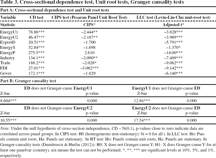
Note: Under the null hypothesis of cross-section independence, CD ∼ N(0,1), p-values close to zero indicate data are correlated across panel groups. In CIPS test: HO (homogeneous non-stationary): bi = 0 for all i. In LLC test: Ho: Panels contain unit roots, Ha: Panels are stationary. In HT test: Ho: Panels contain unit roots, Ha: Panels are stationary. In Granger-causality tests (Dumitrescu & Hurlin (2012)): HO: X does not Granger-cause Y; H1: X does Granger-cause Y for at least one panelvar (country). n/a means the test can not be performed.

*, **, ***

are significant levels at 10%, 5%, and 1%, respectively.

We apply the PCSE model for Eq. [1] with one adjustment to deal with the endogene-ity issue. All independent variables in Eq. [1] are regressed using one-year lags. However, using the PCSE model and one-year lags of independent variables may only partially solve endogeneity. Therefore, we apply the two-step system GMM estimator as a robustness check. The GMM estimator is proposed by Arellano and Bond (1991) and then developed to become system GMM in Arellano and Bover (1995) and two-step system GMM in Blundell and Bond (1998). Two-step system GMM estimator is argued to reduce the bias associated with the fixed effects in short panels (Roodman, 2009). The Feasible Generalized Least Squares (FGLS) (Liao & Cao, 2013; Reed & Ye, 2011; Zhang & Nian, 2013) is also recruited as a robustness estimator to deal with heteroscedasticity in panel data. The study adds control variables one by one to check for the sensitivity of the results. At last, the predictive margins analysis is done for the squared term of ED to illustrate the non-linear impacts of ED on energy use.

4. Results and Discussion

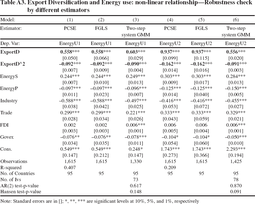
Tables 4 and 5 present the study's main results, while Table A3 in the Appendix reports the robustness check. All results are consistent and robust when each control variable is added to the estimation or by different estimators.

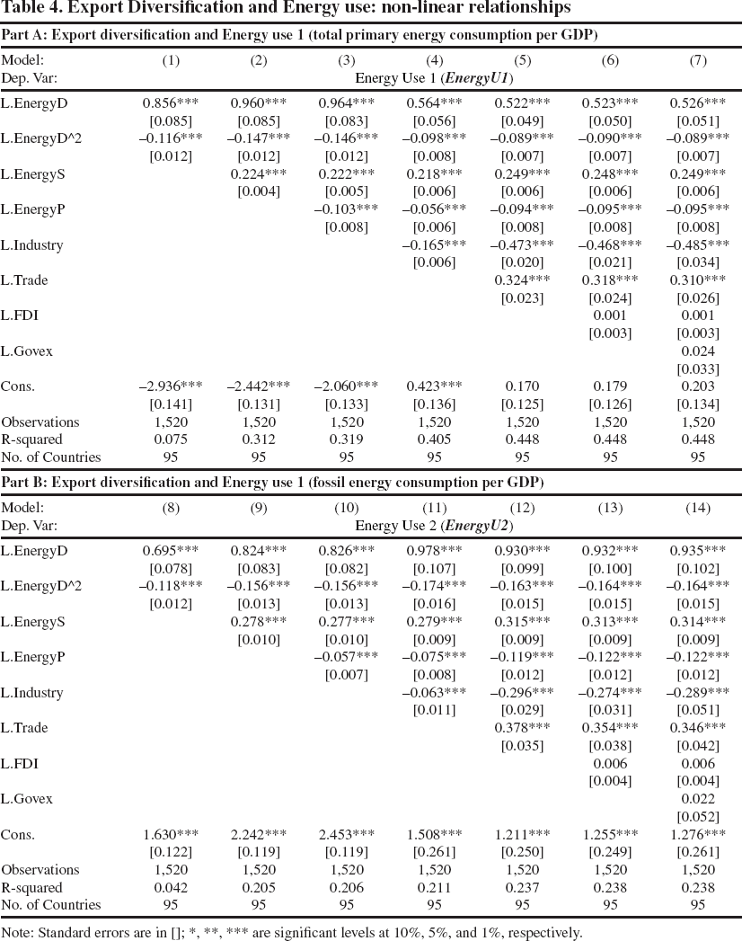
Table 4 reports the impacts of ED on two kinds of energy use, i.e., primary energy consumption per GDP (EnergyUl) in Part A and fossil energy consumption per GDP (EnergyUl) in Part B, in the global sample. In terms of control variables, the energy supply (EnergyS) has significant positive impacts, which implies the increasing effects of a higher energy supply on energy use. The energy price (EnergyP) has a significant negative impact, which means the higher energy price would reduce energy use. These effects are in common wisdom that a higher supply or low price would stimulate the consumption of a product, which is energy. The industry value (Industry) also has a significant negative impact, which suggests that industrialization would reduce energy use per output unit. That is, the increases in industrial sectors would be a more energy efficient one. Trade openness (Trade) and FDI inflows (FDI) have positive impacts but only statistical significance in the case of trade openness. This result implies that higher trade openness may cause higher energy use, while the impacts of FDI are unclear. At last, the government expenditures have positive but also statistically insignificant.

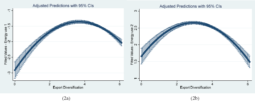
In terms of the main variable, ED has a significant positive impact, while its squared term has significant negative impacts. The results are consistent and robust when each control variable is added. The results are also consistent with different estimations, i.e., PCSE estimator with all independent variables in the current year, FGLS, and two-step system GMM (see Table A3, Appendix, for these results. The results confirm that ED has non-linear impacts on energy use following invert-ed-U shapes. The increases in ED at the initial level would cause higher energy use (or higher energy inefficiency) until a certain level. After that threshold, the increases in ED would help to reduce energy use (or increase energy efficiency). The finding confirms our hypothesis that ED has non-linear influences on energy use following an inverted-U shape. The results are the same for both kinds of energy use (EnergyUl—primary energy consumption per GDP and EnergyU2—fossil energy consumption per GDP). Figure 2, the predictive margins analysis for the impacts of ED on energy use, illustrates these non-linear impacts clearer. Figure 2a illustrates the inverted-U shape impacts of ED on primary energy consumption, and Figure 2b is the case of fossil energy consumption.

The results highlight that the diversification of exports benefits the domestic economy and costs the environment in the initial stage. This finding adds new evidence to the current literature on the non-linear relationship between ED with economic factors such as productivity or income inequality (e.g., see Xuefeng and Yaşar (2016), Le and Nguyen (2019)). The results, on the other hand, highlight an important policy implication. That is, the country with the export-led development strategy in line with export diversification should focus on regulations and supports, especially policies to reduce using fossil energy, for domestic firms in entering new markets or new products, which help reduce initial costs of entry and exposures to global risk. As a result, domestic firms' transformation would lead to low energy-intensive sectors or high technology production. This result will lead to low energy use and environmental protection. Above that, low energy use would improve energy security and stimulate economic growth in the long run (Le & Nguyen, 2019).

Table 4
Export Diversification and Energy use: non-linear relationships

Part A: Export diversification and Energy use 1 (total primary energy consumption per GDP)

Model: (1) (2) (3) (4) (5) (6) (7)

Dep. Var: Energy Use 1 (EnergyUl)

L.EnergyD 0.856* 0.960* 0.964* 0.564* 0.522* 0.523* 0.526*

[0.085] [0.085] [0.083] [0.056] [0.049] [0.050] [0.051]

L.EnergyD^2 -0.116* -0.147* -0.146* -0.098* -0.089* -0.090* -0.089*

[0.012] [0.012] [0.012] [0.008] [0.007] [0.007] [0.007]

L.EnergyS 0.224* 0.222* 0.218* 0.249* 0.248* 0.249*

[0.004] [0.005] [0.006] [0.006] [0.006] [0.006]

L.EnergyP -0.103* -0.056* -0.094* -0.095* -0.095*

[0.008] [0.006] [0.008] [0.008] [0.008]

L. Industry -0.165* -0.473* -0.468* -0.485*

[0.006] [0.020] [0.021] [0.034]

L. Trade 0.324* 0.318* 0.310*

[0.023] [0.024] [0.026]

L.FDI 0.001 0.001

[0.003] [0.003]

L.Govex 0.024

[0.033]

Cons. -2.936* -2.442* -2.060* 0.423* 0.170 0.179 0.203

[0.141] [0.131] [0.133] [0.136] [0.125] [0.126] [0.134]

Observations 1,520 1,520 1,520 1,520 1,520 1,520 1,520

R-squared 0.075 0.312 0.319 0.405 0.448 0.448 0.448

No. of Countries 95 95 95 95 95 95 95

Part B: Export diversification and Energy use 1 (fossil energy consumption per GDP)

Model: (8) (9) (10) (11) (12) (13) (14)

Dep. Var: Energy Use 2 (EnergyUl)

L.EnergyD 0.695* 0.824* 0.826* 0.978* 0.930* 0.932* 0.935*

[0.078] [0.083] [0.082] [0.107] [0.099] [0.100] [0.102]

L.EnergyD^2 -0.118* -0.156* -0.156* -0.174* -0.163* -0.164* -0.164*

[0.012] [0.013] [0.013] [0.016] [0.015] [0.015] [0.015]

L.EnergyS 0.278* 0.277* 0.279* 0.315* 0.313* 0.314*

[0.010] [0.010] [0.009] [0.009] [0.009] [0.009]

L.EnergyP -0.057* -0.075* -0.119* -0.122* -0.122*

[0.007] [0.008] [0.012] [0.012] [0.012]

L. Industry -0.063* -0.296* -0.274* -0.289*

[0.011] [0.029] [0.031] [0.051]

L. Trade 0.378* 0.354* 0.346*

[0.035] [0.038] [0.042]

L.FDI 0.006 0.006

[0.004] [0.004]

L.Govex 0.022

[0.052]

Cons. 1.630* 2.242* 2.453* 1.508* 1.211* 1.255* 1.276***

[0.122] [0.119] [0.119] [0.261] [0.250] [0.249] [0.261]

Observations 1,520 1,520 1,520 1,520 1,520 1,520 1,520

R-squared 0.042 0.205 0.206 0.211 0.237 0.238 0.238

No. of Countries 95 95 95 95 95 95 95

Part A: Export diversification and Energy use 1 (total primary energy consumption per GDP)
L.EnergyD	0.856***	0.960***	0.964***	0.564***	0.522***	0.523***	0.526***
	[0.085]	[0.085]	[0.083]	[0.056]	[0.049]	[0.050]	[0.051]
L.EnergyD^2	-0.116***	-0.147***	-0.146***	-0.098***	-0.089***	-0.090***	-0.089***
	[0.012]	[0.012]	[0.012]	[0.008]	[0.007]	[0.007]	[0.007]
L.EnergyS		0.224***	0.222***	0.218***	0.249***	0.248***	0.249***
		[0.004]	[0.005]	[0.006]	[0.006]	[0.006]	[0.006]
L.EnergyP			-0.103***	-0.056***	-0.094***	-0.095***	-0.095***
			[0.008]	[0.006]	[0.008]	[0.008]	[0.008]
L. Industry				-0.165***	-0.473***	-0.468***	-0.485***
				[0.006]	[0.020]	[0.021]	[0.034]
L. Trade					0.324***	0.318***	0.310***
					[0.023]	[0.024]	[0.026]
L.FDI						0.001	0.001
						[0.003]	[0.003]
L.Govex							0.024
							[0.033]
Cons.	-2.936***	-2.442***	-2.060***	0.423***	0.170	0.179	0.203
	[0.141]	[0.131]	[0.133]	[0.136]	[0.125]	[0.126]	[0.134]
Observations	1,520	1,520	1,520	1,520	1,520	1,520	1,520
R-squared	0.075	0.312	0.319	0.405	0.448	0.448	0.448
No. of Countries	95	95	95	95	95	95	95
Part B: Export diversification and Energy use 1 (fossil energy consumption per GDP)
Model:	(8)	(9)	(10)	(11)	(12)	(13)	(14)
Dep. Var:			Energy Use 2 (EnergyUl)
L.EnergyD	0.695***	0.824***	0.826***	0.978***	0.930***	0.932***	0.935***
	[0.078]	[0.083]	[0.082]	[0.107]	[0.099]	[0.100]	[0.102]
L.EnergyD^2	-0.118***	-0.156***	-0.156***	-0.174***	-0.163***	-0.164***	-0.164***
	[0.012]	[0.013]	[0.013]	[0.016]	[0.015]	[0.015]	[0.015]
L.EnergyS		0.278***	0.277***	0.279***	0.315***	0.313***	0.314***
		[0.010]	[0.010]	[0.009]	[0.009]	[0.009]	[0.009]
L.EnergyP			-0.057***	-0.075***	-0.119***	-0.122***	-0.122***
			[0.007]	[0.008]	[0.012]	[0.012]	[0.012]
L. Industry				-0.063***	-0.296***	-0.274***	-0.289***
				[0.011]	[0.029]	[0.031]	[0.051]
L. Trade					0.378***	0.354***	0.346***
					[0.035]	[0.038]	[0.042]
L.FDI						0.006	0.006
						[0.004]	[0.004]
L.Govex							0.022
							[0.052]
Cons.	1.630***	2.242***	2.453***	1.508***	1.211***	1.255***	1.276***
	[0.122]	[0.119]	[0.119]	[0.261]	[0.250]	[0.249]	[0.261]
Observations	1,520	1,520	1,520	1,520	1,520	1,520	1,520
R-squared	0.042	0.205	0.206	0.211	0.237	0.238	0.238
No. of Countries	95	95	95	95	95	95	95

Note: Standard errors are in []; *, **, *** are significant levels at 10%, 5%, and 1%, respectively.

Next, the estimations for three subsamples are presented in Table 5. In the case of LMEs and UMEs, ED has significant positive impacts, while its squared term has significant negative impacts. This result re-affirms the inverted-U shape impacts of ED on energy use in both LMEs and UMEs. This result makes sense in the case of LMEs and UMEs since they mostly have a low level of technological production and are in the process of industrialization. Export diversification would transform their economic sectors from agricultural to industrial ones.

Table 5

Export Diversification and Energy use: Non-linear relationships in three subsamples

Model:	(1)	(2)	(3)	(4)	(5)	(6)
Groups:	LMEs		UMEs		HIEs
Dep. Var:	EnergyUl	EnergyU2	EnergyUl	EnergyU2	EnergyUl	EnergyU2
ExportD	0.275*	0.698***	0.113	0.237**	-0.218***	-0.450***
	[0.141]	[0.161]	[0.070]	[0.109]	[0.044]	[0.064]
ExportD^2	-0.080***	-0.170***	-0.017*	-0.041***	0.063***	0.105***
	[0.019]	[0.023]	[0.009]	[0.015]	[0.007]	[0.009]
EnergyS	0.336***	0.416***	0.210***	0.187***	0.095***	0.114***
	[0.008]	[0.012]	[0.005]	[0.007]	[0.007]	[0.012]
EnergyP	-0.072***	-0.152***	-0.056***	-0.103***	-0.086***	-0.086***
	[0.022]	[0.032]	[0.009]	[0.016]	[0.009]	[0.009]
Industry	-1.071***	-0.892***	-0.711***	-0.628***	-0.271***	-0.178***
	[0.074]	[0.085]	[0.039]	[0.056]	[0.026]	[0.038]
Trade	0.722***	1.110***	0.349***	0.319***	0.002	-0.154***
	[0.052]	[0.083]	[0.030]	[0.053]	[0.018]	[0.020]
FDI	-0.000	-0.010	0.015***	0.029***	-0.005***	-0.002
	[0.005]	[0.007]	[0.004]	[0.007]	[0.002]	[0.002]
Govex	-0.078**	-0.042	-0.102***	-0.021	-0.237***	-0.232***
	[0.036]	[0.051]	[0.033]	[0.046]	[0.024]	[0.037]
Cons.	0.920**	-2.362***	2.419***	5.362***	4.543***	9.891***
	[0.461]	[0.546]	[0.219]	[0.384]	[0.125]	[0.148]
Observations	512	512	464	464	544	544
R-squared	0.574	0.507	0.329	0.193	0.655	0.571
No. of Countries	32	32	29	29	34	34

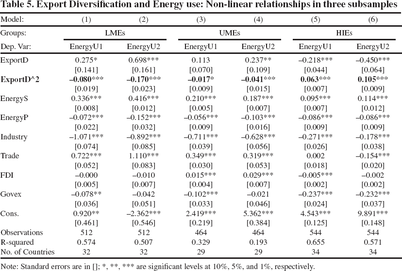
Note: Standard errors are in []; *, **, *** are significant levels at 10%, 5%, and 1%, respectively.

Figure 2

Export Diversification, Export Quality and Energy use: Non-linear evidence

Meanwhile, they are constrained by financial issues by investing vast amounts of money in high-technology production. As a result, they would invest and expand economic activities to high-energy-intensive sectors. This process may be happening until a certain level of ED, where the economics of scale and the relative advancement in their production would turn the impacts of ED on energy use from positive to negative. The results imply that governments in LMEs and UMEs should support ED as much as possible to overcome the threshold, whereas the higher ED would help reduce energy use. Meanwhile, governments in LMEs and UMEs should also provide support to reduce the positive impacts of ED on energy use in the initial phase.

Figure 3

Export Diversification and Energy use in three subsamples: non-linear evidence

In the case of HIEs, there are opposite impacts. ED has a significant negative impact, while its squared term has a significant positive impact. That means ED has a U-shaped impact on energy use in HIEs. This result is very interesting to notice the difference in HIEs and may be explained by the fact that the production of HIEs has already been in high technological advancement. The increases in ED, especially in new markets, would push their firms to international competition.

Meanwhile, the producers in LMEs and UMEs are advanced by low costs of labour, which put back challenges for producers in HIEs in cost savings. In return, they may choose products or sectors with high energy-intensive use to compete since they need help to cut labour wages. As a result, the technological advancement in HIEs can only bring benefits to the environment through decreased energy use when they expand the exports to new products or markets. After a threshold, producers may follow the wisdom of the EKC by focusing on high energy-intensive sectors. As a result, ED would then induce higher energy use in HIEs.

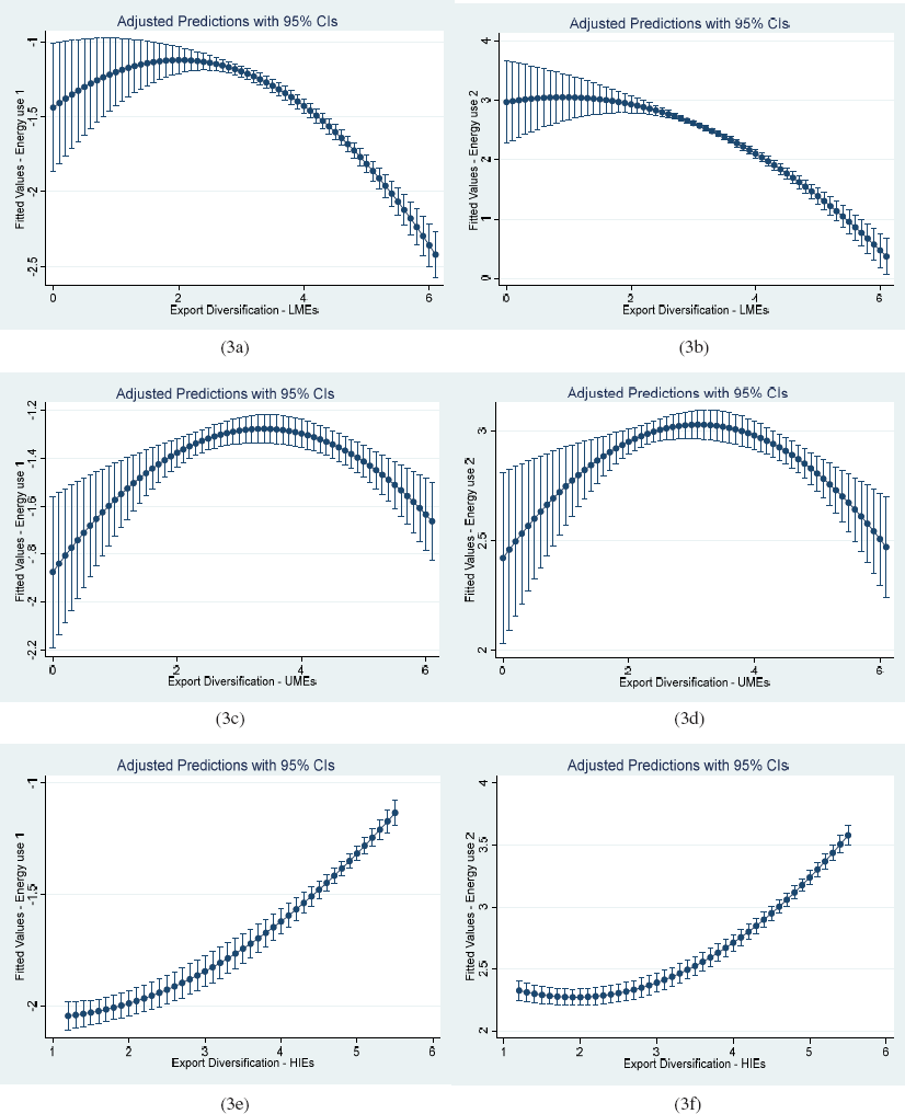
Figure 3 illustrates the predictive margins analysis for the impacts of ED on energy use in three subsamples (Figures 3a and 3b for the LMEs, Figures 3c and 3d for UMEs, and Figures 3e and 3f for HIEs). This result shows a clear inverted-U shape impact of ED on both kinds of energy use in LMEs and UMEs, while it is likely a U-shaped impact of ED on energy use in HIEs. However, the U-shaped impacts in HIEs are not strong ones. That confirms that ED can only bring some short-term benefits in reducing energy use in HIEs.

5. Conclusion

Expanding exports to new markets or products in the process of export diversification brings benefits and costs. On the one hand, ED helps to improve productivity and employment while it creates new economic activities and economic development. On the other hand, ED exposes domestic firms to international risk and high entry costs. That is, ED is likely a process with pros and cons, and it has a non-linear impact on domestic economic activities. In this context, the subject study adds to the existing evidence on the nexus between ED and energy consumption and in so doing, draws on global evidence while accounting for the non-linear impacts of ED on energy use. In light of a comprehensive empirical exercise and results, we conclude on the presence of non-linear linkages between export diversification (ED) and energy consumption. More specifically, we conclude that there is an inverted-U shape ED effect on energy use per output unit. This implies the increases in energy inefficiency in the progress of diversification improvement in exports until a threshold level from which ED would help to enhance energy efficiency. Our analysis of the three subsamples shows consistent findings regarding the effects of ED across income levels. The inverted-U shape effects of ED are consistent in LMEs and UMEs, while it is ambiguous in HIEs. It leads to the further conclusion that low and middle economies should diversify exports as much as possible to pass the threshold, where diversification can improve energy efficiency.

This paper contributes to the existing evidence on export diversification and energy consumption in two main aspects. First, the non-linear impacts of ED on energy consumption are examined and the case for the underlying nexus is established in the light of robust empirical evidence. Second, this relationship is investigated from a very broad global perspective and three subsamples (i.e., LMEs, UMEs, and HIEs) that provide deeper insight while accounting for the heterogeneities in the level of development across countries. The empirical results and the conclusion we have drawn are also robust from the PCSE model and various robustness estimators (i.e., FGLS, two-step system GMM) and estimation strategies (using one-year lags of independent variables and adding each control variable to check for sensitivity). We also conclude on significant Granger causality between ED and both kinds of energy use, including primary energy consumption and fossil energy use. Notably, the inverted-U shape impacts of ED on energy use are documented in global and two subsamples, including LMEs and UMEs. Meanwhile, a U-shape relationship is found in HIEs. Our findings have propounding implications for trade policy and energy policymakers.

Footnotes

Appendix

Table A1.

List of countries

32 Low- and Lower-Middle Income Economies (LMEs)
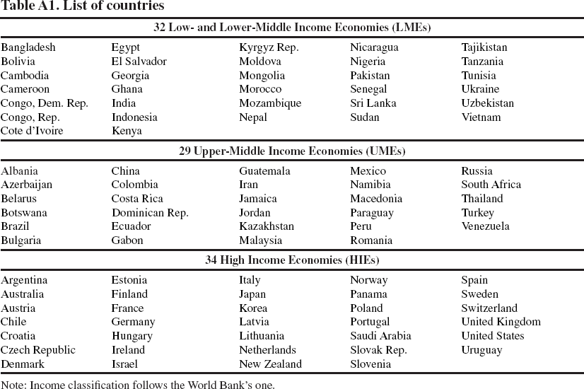
Bangladesh	Egypt	Kyrgyz Rep.	Nicaragua	Tajikistan
Bolivia	El Salvador	Moldova	Nigeria	Tanzania
Cambodia	Georgia	Mongolia	Pakistan	Tunisia
Cameroon	Ghana	Morocco	Senegal	Ukraine
Congo, Dem. Rep.	India	Mozambique	Sri Lanka	Uzbekistan
Congo, Rep.	Indonesia	Nepal	Sudan	Vietnam
Cote d, Ivoire	Kenya
29 Upper-Middle Income Economies (UMEs)
Albania	China	Guatemala	Mexico	Russia
Azerbaijan	Colombia	Iran	Namibia	South Africa
Belarus	Costa Rica	Jamaica	Macedonia	Thailand
Botswana	Dominican Rep.	Jordan	Paraguay	Turkey
Brazil	Ecuador	Kazakhstan	Peru	Venezuela
Bulgaria	Gabon	Malaysia	Romania
34 High Income Economies (HIEs)
Argentina	Estonia	Italy	Norway	Spain
Australia	Finland	Japan	Panama	Sweden
Austria	France	Korea	Poland	Switzerland
Chile	Germany	Latvia	Portugal	United Kingdom
Croatia	Hungary	Lithuania	Saudi Arabia	United States
Czech Republic	Ireland	Netherlands	Slovak Rep.	Uruguay
Denmark	Israel	New Zealand	Slovenia

Note: Income classification follows the World Bank's one.

Table A2.

Data description of three subsamples

Variable	Obs	Mean	SD.	Min	Max
32 LMEs
Energy U1	544	-1.371	0.876	-3.156	0.979
EnergyU2	544	2.285	1.501	-1.418	5.571
ExportD	544	3.479	1.038	0.000	6.038
EnergyS	544	-1.918	1.710	-6.843	1.179
EnergyP	544	3.915	0.615	2.669	4.602
Industry	544	10.357	0.823	8.184	12.259
Trade	544	11.328	0.874	8.842	13.025
FDI	544	3.838	4.896	-4.844	43.912
Govex	544	9.552	0.902	6.392	11.268
29 UMEs
Energy U1	493	-1.35	0.60	-2.61	0.47
EnergyU2	493	2.94	0.82	0.40	5.06
ExportD	493	3.23	1.19	0.00	6.06
EnergyS	493	-1.78	1.50	-6.27	0.58
EnergyP	493	3.92	0.62	2.67	4.60
Industry	493	12.05	0.59	10.25	13.52
Trade	493	12.84	0.60	10.82	14.33
FDI	493	4.26	5.32	-5.84	55.08
Govex	493	11.22	0.57	9.40	12.32
34 HIEs
Energy U1	578	-1.94	0.46	-2.95	-0.87
EnergyU2	578	2.34	0.57	0.55	3.69
ExportD	578	2.21	0.75	1.29	5.47
EnergyS	578	-2.91	1.45	-9.12	0.39
EnergyP	578	3.92	0.62	2.67	4.60
Industry	578	13.38	0.72	11.49	15.11
Trade	578	14.42	0.78	12.04	16.11
FDI	578	4.75	6.98	-15.99	87.44
Govex	578	13.02	0.80	11.12	14.46

Table A3.

Export Diversification and Energy use: non-linear relationship—Robustness check by different estimators

Model:	(1)	(2)	(3)	(4)	(5)	(6)
Estimator:	PCSE	FGLS	Two-step system GMM	PCSE	FGLS	Two-step system GMM
Dep. Var:	Energy U1	Energy U1	Energy U1	EnergyU2	EnergyU2	EnergyU2
ExportD	0.558***	0.558***	0.603***	0.937***	0.937***	0.556***
	[0.050]	[0.066]	[0.029]	[0.099]	[0.115]	[0.020]
ExportD^2	-0.092***	-0.092***	-0.090***	-0.162***	-0.162***	-0.091***
	[0.007]	[0.009]	[0.004]	[0.014]	[0.016]	[0.003]
EnergyS	0.244***	0.244***	0.249***	0.303***	0.303***	0.284***
	[0.007]	[0.010]	[0.013]	[0.009]	[0.017]	[0.013]
EnergyP	-0.097***	-0.097***	-0.096***	-0.125***	-0.125***	-0.150***
	[0.011]	[0.023]	[0.007]	[0.014]	[0.040]	[0.005]
Industry	-0.588***	-0.588***	-0.497***	-0.416***	-0.416***	-0.455***
	[0.038]	[0.042]	[0.025]	[0.053]	[0.072]	[0.027]
Trade	0.299***	0.299***	0.221***	0.333***	0.333***	0.329***
	[0.028]	[0.034]	[0.026]	[0.043]	[0.059]	[0.021]
FDI	0.002	0.002	0.006***	0.006	0.006	0.006***
	[0.003]	[0.003]	[0.001]	[0.005]	[0.004]	[0.001]
Govex	-0.076**	-0.076**	-0.078***	-0.104*	-0.104*	-0.050***
	[0.034]	[0.035]	[0.011]	[0.054]	[0.060]	[0.010]
Cons.	0.549***	0.549***	0.248*	1.743***	1.743***	2.293***
	[0.147]	[0.212]	[0.147]	[0.273]	[0.366]	[0.194]
Observations	1,615	1,615	1,330	1,615	1,615	1,425
R-squared	0.407			0.209
No. of Countries	95	95	95	95	95	95
No. of Ivs			73			78
AR(2) test-p-value			0.617			0.870
Hansen test-p-value			0.148			0.091

Note: Standard errors are in []; *, **, *** are significant levels at 10%, 5%, and 1%, respectively

References

Adom

P.K.

and Adams

(2018). "Energy savings in Nigeria. Is there a way of escape from energy inefficiency?" Renewable and Sustainable Energy Reviews 81: 2421–2430. https://doi.org/10.1016/j.rser.2017.06.048

Albassam

B.A

. (2015). "Economic diversification in Saudi Arabia: Myth or reality?" Resources Policy 44: 112–117. https://doi.org/10.1016/j.resourpol.2015.02.005

Arellano

and Bond

(1991). "Some tests of specification for panel data: Monte Carlo evidence and an application to employment equations." The review of economic studies 58 (2) 277–297.

Arellano

and Bover

(1995). "Another look at the instrumental variable estimation of error-components models." Journal of Econometrics 68 (1) 29–51. http://dx.doi.org/l0.1016/0304-4076 (94)01642-D

B.Y.

and Lee

(2017). "Demand, costs and product scope in the export market." European Economic Review 100: 28–49. https://doi.org/10.1016/j.euroecorev.2017.07.009

Azadi

Verheijke

, and Witlox

(2011). "Pollute first, clean up later?" Global and Planetary Change 78 (3-4): 77–82.

Azam

Khan

A.Q.

Zaman

, and Ahmad

(2015). "Factors determining energy consumption: Evidence from Indonesia, Malaysia and Thailand." Renewable and Sustainable Energy Reviews 42: 1123–1131. https://doi.org/10.1016/j.rser.2014.10.061

Bailey

and Katz

J.N.

(2011). "Implementing Panel Corrected Standard Errors in R: The pcse Package." Journal of Statistical Software 42(CS1): 1–11.

Bashir

M.A.

Sheng

Doğan

Sarwar

, and Shahzad

(2020). "Export product diversification and energy efficiency: Empirical evidence from OECD countries." Structural Change and Economic Dynamics 55: 232–243. https://doi.org/10.1016/j.strueco.2020.09.002

10.

Blundell

and Bond

(1998). "Initial conditions and moment restrictions in dynamic panel data models." Journal of econometrics 87 (1) 115–143.

11.

Bye

B., T.

Fœhn

, and Rosnes

(2018). "Residential energy efficiency policies: Costs, emissions and rebound effects." Energy 143: 191–201. https://doi.org/10.1016/j.energy.2017.10.103

12.

Canh

N. P

Schinckus

, and Thanh

S.D.

(2019). "Do economic openness and institutional quality influence patents? Evidence from GMM systems estimates." International Economics 157: 134–169.

13.

Canh

N. P

Thanh

S.D.

, and Nasir

M.A.

(2020). "Nexus between financial development & energy intensity: Two sides of a coin?" Journal of Environmental Management 210: 110902. https://doi.org/10.1016/j.jenvman.2020.110902

14.

Canh

N. P

Thanh

S.D.

Schinckus

Bensemann

, and Thanh

L.T.

(2019). "Global Emissions: A New Contribution from the Shadow Economy." International Journal of Energy Economics and Policy 9 (3) 320–337.

15.

Canh

P.N.

and Thanh

S. Dinh

(2020). "Exports and the shadow economy: Non-linear effects." The Journal of International Trade & Economic Development 29 (7) 865–890. https://doi.org/10.1080/09638199.2020.1759676

16.

Chen

and Lei

(2018). "The impacts of renewable energy and technological innovation on environment-energy-growth nexus: New evidence from a panel quantile regression." Renewable Energy 123: 1–14. https://doi.org/10.1016/j.renene.2018.02.026

17.

Chen

(2018). "Factors influencing renewable energy consumption in China: An empirical analysis based on provincial panel data." Journal of Cleaner Production 174: 605–615. https://doi.org/10.1016/j.jclepro.2017.11.011

18.

Contractor

F.J.

and Kundu

(2004). "The role of export-driven entrepreneurship in economic development: A comparison of software exports from India, China, and Taiwan." Technological Forecasting and Social Change 71 (8) 799–822. https://doi.org/10.1016/j.techfore.2004.01.012

19.

Dietz

and Rosa

E.A.

(1997). "Effects of population and affluence on CO2 emissions." Proceedings of the National Academy of Sciences 94 (1) 175–179.

20.

Dumitrescu

E.-I.

and Hurlin

(2012). "Testing for Granger non-causality in heterogeneous panels." Economic Modelling 29 (4) 1450–1460.

21.

Egger

and Etzel

(2012). "The impact of trade on employment, welfare, and income distribution in unionized general oligopolistic equilibrium." European Economic Review 56 (6) 1119–1135. https://doi.org/10.1016/j.euroecorev.2012.03.006

22.

Ehrlich

PR.

and Holdren

J. P

(1971). "Impact of population growth." Science 171 (3977) 1212–1217.

23.

Fillat

J.L.

Garetto

, and Oldenski

(2015). "Diversification, cost structure, and the risk premium of multinational corporations." Journal of International Economics 96 (1) 37–54. https://doi.org/10.1016/j.jinteco.2015.01.004

24.

Hanif

(2018). "Impact of fossil fuels energy consumption, energy policies, and urban sprawl on carbon emissions in East Asia and the Pacific: A panel investigation." Energy Strategy Reviews 21: 16–24. https://doi.org/10.1016/j.esr.2018.04.006

25.

Hoffman

R.C.

Munemo

, and Watson

(2016). "International Franchise Expansion: The Role of Institutions and Transaction Costs." Journal of International Management 22 (2) 101–114. https://doi.org/http://dx.doi.org/10.1016/j.intman.2016.01.003

26.

Jiang

and Lin

(2012). "China's energy demand and its characteristics in the industrialization and urbanization process." Energy policy 49: 608–615.

27.

Jones

M.V.

Coviello

, and Tang

Y.K.

(2011). "International Entrepreneurship research (1989-2009): A domain ontology and thematic analysis." Journal of Business Venturing 26 (6) 632–659. https://doi.org/10.1016/j.jbusvent.2011.04.001

28.

Jönsson

(2005). "Cross-sectional Dependency and Size Distortion in a Small-sample Homogeneous Panel Data Unit Root Test." Oxford Bulletin of Economics and Statistics 67 (3) 369–392.

29.

Kasman

and Duman

Y.S.

(2015). "C02 emissions, economic growth, energy consumption, trade and urbanization in new EU member and candidate countries: a panel data analysis." Economic Modelling 44: 97–103.

30.

T.-H.

and Nguyen

C.P.

(2019). "Is energy security a driver for economic growth? Evidence from a global sample." Energy policy 129: 436–451.

31.

T.-H.

Nguyen

C.P.

TD.

, and Tran-Nam

(2020). "The Kuznets curve for export diversification and income inequality: Evidence from a global sample." Economic Analysis and Policy 65: 21–39. https://doi.org/10.1016/j.eap.2019.11.004

32.

Levin

Lin

C.-F.

, and Chu

C.-S.J.

(2002). "Unit root tests in panel data: asymptotic and finite-sample properties." Journal of econometrics 108 (1) 1–24.

33.

Liao

and Cao

H.-S.

(2013). "How does carbon dioxide emission change with the economic development? Statistical experiences from 132 countries." Global Environmental Change 23 (5) 1073–1082.

34.

Lin

and Zhu

(2017). "Energy and carbon intensity in China during the urbanization and industrialization process: A panel VAR approach." Journal of Cleaner Production 168: 780–790. https://doi.org/10.1016/j.jclepro.2017.09.013

35.

Marques

A.C.

and Fuinhas

J.A.

(2012). "Is renewable energy effective in promoting growth?" Energy Policy 46: 434–442.

36.

Nguyen

C. P

Nguyen

N.A.

Schinckus

, and Su

TD.

(2018). "The Ambivalent Role of Institutions in the CO2 Emissions: The Case of Emerging Countries." International Journal of Energy Economics and Policy 8 (5) 7–17.

37.

Njikam

(2017). "Export market destination and performance: Firm-level evidence from Sub-Saharan Africa." Journal of African Trade 4 (1) 1–19. https://doi.org/10.1016/j.joat.2018.01.001

38.

Omri

and Nguyen

D.K.

(2014). "On the determinants of renewable energy consumption: International evidence." Energy 72: 554–560.

39.

Osakwe

P.N.

Santos-Paulino

A.U.

, and Dogan

(2018). "Trade dependence, liberalization, and exports diversification in developing countries." Journal of African Trade 5 (1) 19–34. https://doi.org/10.1016/j.joat.2018.09.001

40.

Pesaran

M.H

. (2004). General diagnostic tests for cross section dependence in panels.

41.

Pesaran

M.H

. (2007). "A simple panel unit root test in the presence of cross-section dependence." Journal of applied econometrics 22 (2) 265–312.

42.

Phuc

Nguyen C.

Schinckus

, and Dinh

Su T.

(2019). "Economic integration and CO2 emissions: evidence from emerging economies." Climate and Development 1–16.

43.

Rashid Gill

, Viswanathan

K.K.

, and Hassan

(2018). "The Environmental Kuznets Curve (EKC) and the environmental problem of the day." Renewable and Sustainable Energy Reviews 81:1636–1642. https://doi.org/10.1016/j.rser.2017.05.247

44.

Reed

W.R.

and Ye

(2011). "Which panel data estimator should I use?" Applied economics 43 (8) 985–1000.

45.

Rock

M.T.

and Angel

D. P

(2007). "Grow First, Clean up Later? Industrial Transformation in East Asia." Environment: Science and Policy for Sustainable Development 49 (4) 8–19.

46.

Roodman

(2009). "How to do xtabond2: An introduction to difference and system GMM in Stata." The Stata Journal 9 (1) 86–136.

47.

Sadorsky

(2013). "Do urbanization and industrialization affect energy intensity in developing countries?" Energy Economics 37: 52–59.

48.

Saidi

Rahman

M.M.

, and Amamri

(2017). "The causal nexus between economic growth and energy consumption: New evidence from global panel of 53 countries." Sustainable Cities and Society 33: 45–56. https://doi.org/10.1016/j.scs.2017.05.013

49.

Schrank

(2005). "Entrepreneurship, export diversification, and economic reform: The birth of a developmental community in the Dominican Republic." Comparative Politics 43–62.

50.

Shahbaz

Gozgor

, and Hammoudeh

(2019). "Human capital and export diversification as new determinants of energy demand in the United States." Energy Economics 78: 335–349. https://doi.org/10.1016/j.eneco.2018.11.016

51.

Sun

(1999). "The nature of CO2 emission Kuznets curve." Energy policy 27 (12) 691–694.

52.

Tiba

and Frikha

(2018). "Income, trade openness and energy interactions: Evidence from simultaneous equation modeling." Energy 147: 799–811. https://doi.org/10.1016/j.energy.2018.01.013

53.

UN (2020). About the Sustainable Development Goals. United Nations. Retrieved 27Mar from https://www.un.org/sustainabledevelopment/sustainable-development-goals/

54.

Vannoorenberghe

Wang

, and Yu

(2016). "Volatility and diversification of exports: Firm-level theory and evidence." European Economic Review 89: 216–247. https://doi.org/10.1016/j.euroecorev.2016.07.002

55.

Xuefeng

and Yaşar

(2016). "Export Market Diversification and Firm Productivity: Evidence from a Large Developing Country." World Development 82: 28–47. https://doi.org/10.1016/j.worlddev.2016.01.017

56.

Zang

Zhao

Wang

, and Guo

(2017). "The effects of urbanization and household-related factors on residential direct CO2 emissions in Shanxi, China from 1995 to 2014: A decomposition analysis." Atmospheric Pollution Research 8 (2) 297–309.

57.

Zhang

and Nian

(2013). "Panel estimation for transport sector CO2 emissions and its affecting factors: A regional analysis in China." Energy Policy 63: 918–926.

Supplementary Material

Please find the following supplemental material available below.

For Open Access articles published under a Creative Commons License, all supplemental material carries the same license as the article it is associated with.

For non-Open Access articles published, all supplemental material carries a non-exclusive license, and permission requests for re-use of supplemental material or any part of supplemental material shall be sent directly to the copyright owner as specified in the copyright notice associated with the article.

0.00 MB

0.03 MB

Part A: Export diversification and Energy use 1 (total primary energy consumption per GDP)
Model:	(1)	(2)	(3)	(4)	(5)	(6)	(7)
Dep. Var:			Energy Use 1 (EnergyUl)
L.EnergyD	0.856***	0.960***	0.964***	0.564***	0.522***	0.523***	0.526***
	[0.085]	[0.085]	[0.083]	[0.056]	[0.049]	[0.050]	[0.051]
L.EnergyD^2	-0.116***	-0.147***	-0.146***	-0.098***	-0.089***	-0.090***	-0.089***
	[0.012]	[0.012]	[0.012]	[0.008]	[0.007]	[0.007]	[0.007]
L.EnergyS		0.224***	0.222***	0.218***	0.249***	0.248***	0.249***
		[0.004]	[0.005]	[0.006]	[0.006]	[0.006]	[0.006]
L.EnergyP			-0.103***	-0.056***	-0.094***	-0.095***	-0.095***
			[0.008]	[0.006]	[0.008]	[0.008]	[0.008]
L. Industry				-0.165***	-0.473***	-0.468***	-0.485***
				[0.006]	[0.020]	[0.021]	[0.034]
L. Trade					0.324***	0.318***	0.310***
					[0.023]	[0.024]	[0.026]
L.FDI						0.001	0.001
						[0.003]	[0.003]
L.Govex							0.024
							[0.033]
Cons.	-2.936***	-2.442***	-2.060***	0.423***	0.170	0.179	0.203
	[0.141]	[0.131]	[0.133]	[0.136]	[0.125]	[0.126]	[0.134]
Observations	1,520	1,520	1,520	1,520	1,520	1,520	1,520
R-squared	0.075	0.312	0.319	0.405	0.448	0.448	0.448
No. of Countries	95	95	95	95	95	95	95
Part B: Export diversification and Energy use 1 (fossil energy consumption per GDP)
Model:	(8)	(9)	(10)	(11)	(12)	(13)	(14)
Dep. Var:			Energy Use 2 (EnergyUl)
L.EnergyD	0.695***	0.824***	0.826***	0.978***	0.930***	0.932***	0.935***
	[0.078]	[0.083]	[0.082]	[0.107]	[0.099]	[0.100]	[0.102]
L.EnergyD^2	-0.118***	-0.156***	-0.156***	-0.174***	-0.163***	-0.164***	-0.164***
	[0.012]	[0.013]	[0.013]	[0.016]	[0.015]	[0.015]	[0.015]
L.EnergyS		0.278***	0.277***	0.279***	0.315***	0.313***	0.314***
		[0.010]	[0.010]	[0.009]	[0.009]	[0.009]	[0.009]
L.EnergyP			-0.057***	-0.075***	-0.119***	-0.122***	-0.122***
			[0.007]	[0.008]	[0.012]	[0.012]	[0.012]
L. Industry				-0.063***	-0.296***	-0.274***	-0.289***
				[0.011]	[0.029]	[0.031]	[0.051]
L. Trade					0.378***	0.354***	0.346***
					[0.035]	[0.038]	[0.042]
L.FDI						0.006	0.006
						[0.004]	[0.004]
L.Govex							0.022
							[0.052]
Cons.	1.630***	2.242***	2.453***	1.508***	1.211***	1.255***	1.276***
	[0.122]	[0.119]	[0.119]	[0.261]	[0.250]	[0.249]	[0.261]
Observations	1,520	1,520	1,520	1,520	1,520	1,520	1,520
R-squared	0.042	0.205	0.206	0.211	0.237	0.238	0.238
No. of Countries	95	95	95	95	95	95	95

Export Diversification and Energy Consumption Efficiency in the Light of Non-linear Evidence

Abstract

Keywords

1. Introduction

1. The Export Diversification measures the export product diversification (see https://www.imf.org/external/np/res/dfidimfydiversification.htm)

3. Methodology and Data

Footnotes

Appendix

References

Supplementary Material

1.
The Export Diversification measures the export product diversification (see https://www.imf.org/external/np/res/dfidimfydiversification.htm)