CB-SEM Latent Interaction: Unconstrained and Orthogonalized Approaches *

Abstract

Covariance Based – Structural Equation Modelling (CB-SEM) is often used to investigate moderation and latent interaction effects. This study illustrates and compares the application of constrained, unconstrained and orthogonalized CB-SEM approaches to latent variable interaction analysis using AMOS. Although all three techniques provided similar parameter estimates, the orthogonalized approach provided reduced standard errors resulting in identifying a significant latent interaction, suggesting the orthogonalized approach may be better suited for exploratory research.

The illustrated example demonstrates three CB-SEM techniques, and the simplicity of the three approaches to test for interaction effects. The three approaches can be comfortably implemented in available software programs. Guidelines and recommendations for the use of the three approaches are identified with a step-wise process of assessing the latent interaction effect in CB-SEM.

As far as we are aware this is the first investigation comparing and recommending specific CB-SEM latent variable moderation analysis techniques in marketing research.

Keywords

Latent Interaction Effects Structural Equation Modelling Unconstrained Approach Orthogonalized Approach Theory of Planned Behavior

1. Introduction

To estimate complex heterogeneity effects, Covariance Based – Structural Equation Modelling (CB-SEM) is often used to investigate moderation and latent interaction effects (e.g., Nunkoo, Ramkissoon, & Gursoy, 2013). Moderation analysis generally takes the form of multi-group analysis for categorical data, (e.g., gender) or creating and analysing subgroups from continuous moderator variables (e.g., level of knowledge) (Baron & Kenny, 1986; Nuzzo, 2019). When the moderating variable is continuous, the assessment and interpretation of moderation using multi-group analysis may be undermined by problems which researchers may not recognize or understand (Dwyer, Gill, & Seetaram, 2012; Okazaki, Li, & Hirose, 2009). Many researchers using CB-SEM follow a common (yet suboptimal) practice of artificially categorizing continuous moderating variables into subgroups, such as ‘‘high’’ and ‘‘low’’ based on whether the cases fall above or below the median of the moderators (Luo, Song, Marnburg, & Øgaard, 2014; Tang & Jang, 2014). This practice results in a loss of information; compromises the interpretation and reduces the variance of the moderators causing the estimated moderating effects to be downward biased and inevitably results in Type I and Type II errors (Aguinis, Edwards, & Bradley, 2017; Dawson, 2014; MacCallum, Zhang, Preacher, & Rucker, 2002). However, when a categorical variable is used as a moderator, then multi-group analysis would be appropriate.

As an alternative, structural equation modelling (SEM) measures latent constructs at the observation level (measurement model), simultaneously testing hypothesized relationships between constructs within a single framework (structural model) and identifies measurement error when estimating the moderator effect (Dwyer et al., 2012; Hair, Black, Babin, & Andersen, 2010; Hair, Sarstedt, Ringle, & Mena, 2012). This approach multiplies the indicators of the latent variables (independent variables) to create moderator variable indicators which measures the interaction term in the path model (Kenny & Judd, 1984). This provides a strong basis for evaluating the underlying factor structure relating multiple indicators to their factors, controlling measurement error, increasing statistical power, testing the implicit factor structure used to create scale scores, and ultimately providing a more defensible interpretation of the interaction effects (Marsh, Wen, & Hau, 2006).

There are three well-documented approaches to latent interaction modelling in CB-SEM, the constrained approach (Algina & Moulder, 2001; Jöreskog & Yang, 1996), the unconstrained approach (Marsh, Hau, & Wen, 2004; Marsh et al., 2006), and the orthogonalized approach (Little, Bovaird, & Widaman, 2006).

Although other studies compare and discuss advantages and disadvantages of different approaches to latent interactions, the purpose and unique contribution of this paper is: 1) Illustrate and compare the application of the constrained, unconstrained and orthogonalized approaches to CB-SEM moderation analysis techniques in recent marketing literature, 2) demonstrate the step by step process to undertake the different approaches, and 3) provide clear guidelines and recommendations for the use and analysis of latent interaction effects. A marketing study using the Theory Planned Behavior (TPB) is used as an illustrative example comparing the constrained, unconstrained and orthogonalized approaches. The unique contribution of the paper are the recommendations and guidelines for the selection of appropriate estimation methods included in the final section to help researchers identify, based on their research goals, an appropriate CB-SEM latent interaction analysis approach.

2. Background and review of estimation methods for latent variable interaction

2.1. Systematic literature review, sources and search strategy

To examine how SEM methods have been applied to research methodology in marketing a systematic literature review covering the years 2009 to 2019 was conducted using the Web of Science (WoS) data bases.

The Preferred Reporting Items for Systematic Reviews (PRISMA) guidelines were used to identify, select, and critically appraise the relevant research search (see Appendix A) (Moher, Liberati, Tetzlaff, & Altman, 2009). The review was restricted to Business research articles published in English, with non-academic publications (i.e., conference papers, book chapters, and book series) excluded. The search criteria included the terms; factor-based SEM OR factor based SEM OR covariance-based SEM OR covariance based SEM OR SEM OR CB-SEM OR latent interaction approach OR latent interaction OR moderator.

2.2. Systematic literature review results

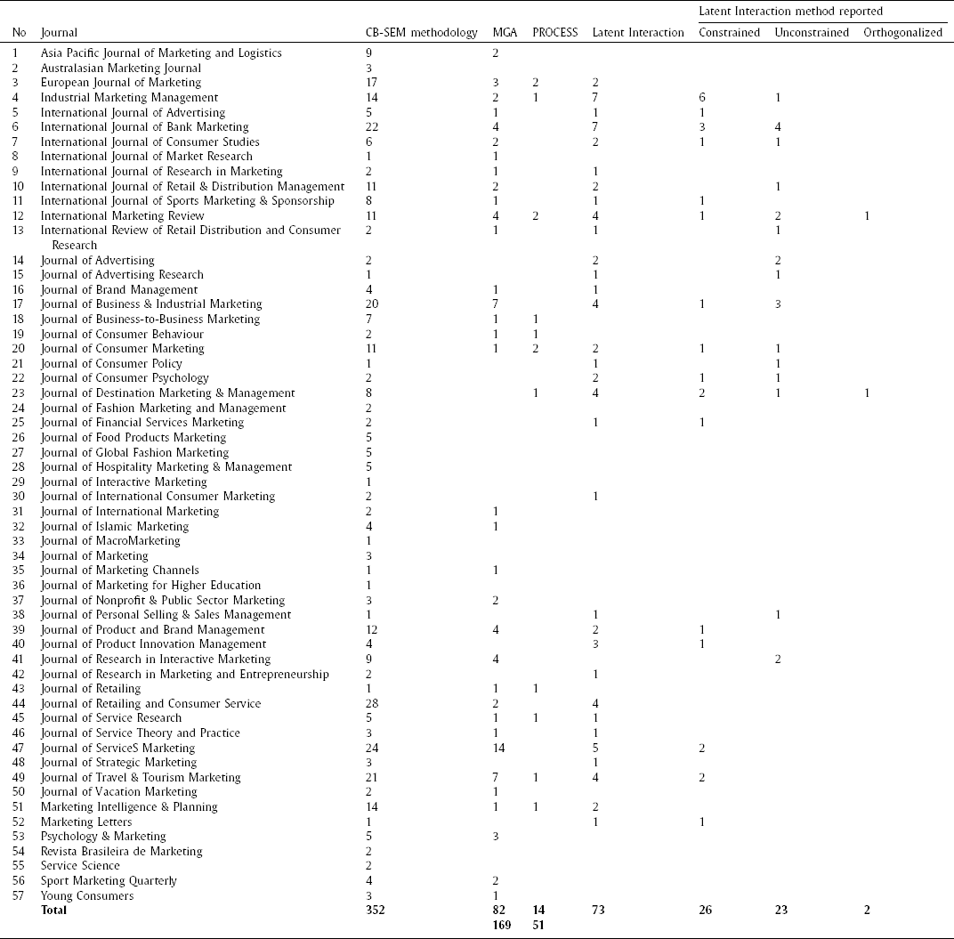
The initial search extracted 2,563 articles from the WoS databases. From this initial extraction 1,817 non-marketing articles were excluded. The remaining 746 articles were examined to ensure they met the criteria (reported using CB-SEM methodology). As a result, 394 articles were excluded for not using CB-SEM, and 352 CB-SEM articles remained for analysis. Of the 352 articles 183 articles were considered tutorial/guideline articles that did not disclose details of moderator assessment and were excluded. The list of journals from which the 169 remaining articles were extracted and used in the analysis are presented in Appendix B.

Despite being an established statistical technique in marketing studies, the execution of latent interaction analysis using CB-SEM is rarely reported by researchers. An analysis of the 169 marketing articles reported using CB-SEM identified 82 articles using multi-group analysis, 14 using CB-SEM and Hayes PROCESS and 73 reporting latent interactions techniques. Twenty-two articles reporting a latent interaction approach were not explained in enough detail to establish the specific analysis technique, implying that a mean-centred computed latent variable score was not considered against an indicator level mean centre approach for the interaction term. Fifty-one articles mentioned the details of the latent interaction approach, the majority reported using the constrained (n = 26) approach, 23 using the unconstrained approach and 2 reported using the orthogonal approach.

2.3. Background and review of latent variable interaction estimation methods

Utilizing the computed latent variable interaction term in CB-SEM may result in factor indeterminacy (Grice, 2001). Factor indeterminacy produces more than one solution that is mathematically sound without providing a means to determine which of the several solutions corresponds to the hypothesis being tested. Therefore, using an interaction term in a computed latent variable score in CB-SEM tends to increase the influence of factor indeterminacy, or random variance, weakening the relationship with the external criterion and explanatory accuracy (Diamantopoulos, Sarstedt, Fuchs, Wilczynski, & Kaiser, 2012). This is not a concern if the mean-centre approach is taken at the indicator level of the interaction term and used in the parameter estimation of the structural relationships.

The SEM approach provides superior results when investigating latent variable interaction with continuous measured moderators, regardless of differences in procedures or techniques (Arminger & Muthén, 1998; Coenders, Lubbers, Scheepers, & Verkuyten, 2008; Klein & Moosbrugger, 2000; Yang-Wallentin & Jöreskog, 2001). Notwithstanding the superiority of the latent interaction approach when using CB-SEM, the number of articles published in marketing journals using this approach suggest that researchers would benefit from a review of the constrained, unconstrained, and orthogonalized approaches.

Although the constrained approach is the most widely used method for latent variable interactions analysis it involves nonlinear constraint requirements used to specify the factor loadings and variances associated with the interaction term (Algina & Moulder, 2001). In particular, some parameters are constrained to have fixed constant values (e.g., 0), whereas others are freely estimated in the SEM analysis. Constraints determine which parameters of the measurement model of the product latent variable (e.g., loadings of the indicators and error (co)variances) are not freely estimated but expressed in terms of the parameters of the measurement models of the first-order effect variables. Importantly, these constraints are typically based on the assumption that latent variables must achieve normal distribution.

Hayduk (1987) implemented Kenny and Judd's (1984) suggested classical constrained technique using LISREL, but the complicated model specification was ambiguous and impractical to use by most researchers. A decade later, Jöreskog and Yang (1996) provided a general model for the specification of constraints, which relied on uncentered indicators – indicators were used in their original format and the mean of the latent interaction were not centred at zero. The inclusion of the constant intercept term in their model considered additional derived nonlinear constraints under the assumption of multivariate normality. Specifically, these constraints are;

1.
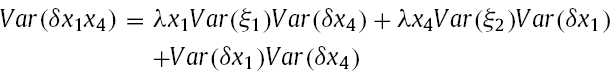
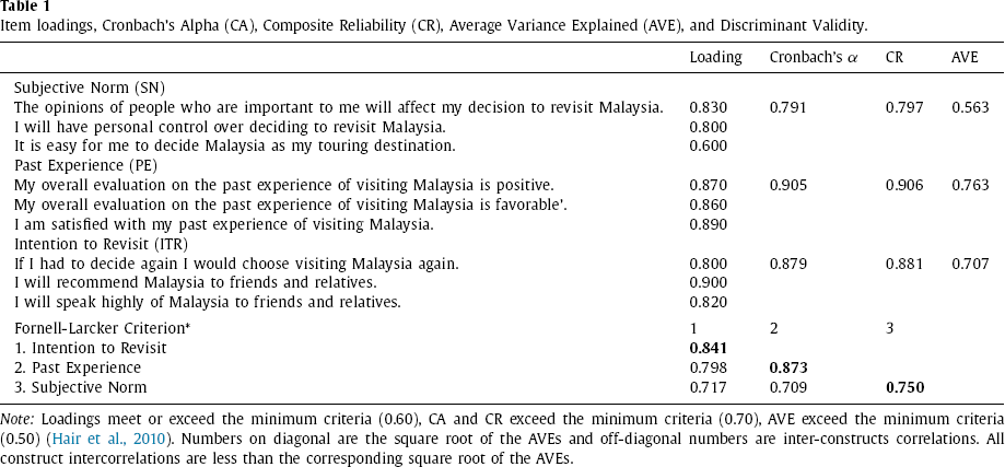
Factor loadings of the product indicators on latent interaction term, for example;

λx1x4 = λx1λx4
2.
Mean of latent interaction term, for example;

E (ξ1ξ2) = Cov (ξ1ξ2)
3.
Variance of latent interaction term, for example;

Var (ξ1ξ2) = Var (ξ1)Var (ξ2) + Cov²(ξ1, ξ2)
4.
Covariance of individual latent factors with latent interaction term, for example;

Cov (ξ1, ξ1ξ2) = Cov (ξ2, ξ1ξ2) = 0
5.
Variance of the unique factors of the product indicators, for example;
$\begin{matrix} V a r (δ x_{1} x_{4}) = λ x_{1} V a r (ξ_{1}) V a r (δ x_{4}) + λ x_{4} (ξ_{2}) V a r (δ x_{1}) \\ + V a r (δ x_{1}) V a r (δ x_{4}) \end{matrix}$

6.
Zero covariances between the unique factors of exogenous indicators and those of product indicators (assuming zero covariances among the unique factors of exogenous indicators)
7.
Covariances between unique factors of product indicators that share the same exogenous indicators (assuming zero covariances among the unique factors of exogenous indicators), for example;
$C o v (δ x_{1} x_{4}, δ x_{1} x_{5}) = λ x_{4} x_{5} V a r (ξ 1) V a r (ξ 2)$

Algina and Moulder (2001) revised and simplified the Jöreskog-Yang model by mean-centring the indicators, which allows the researchers to ignore the intercepts and latent means (at least of the first-order effect variables) to improve the interpretability of the estimates. The coefficient value for a mean-centred predictor would be more practically meaningful than the same coefficient for the same predictor with an arbitrary zero point (i.e., interpreting the relative size of change in Y for a one-unit m change in X at a given level of Z may be easier if the zero point of Z is the average value of Z rather than an arbitrary and non-meaningful scale value). The interpretation may also be improved by plotting the predicted relation between X and Y over a range of plausible z scores (e.g., Aiken & West, 1991; Cohen, Cohen, West, & Aikken, 2003; Mossholder, Kemery, & Bedeian, 1990). In addition, the use of mean-centring eases the ill conditioning of the correlation matrix among the predictors that results from nonessential multicollinearity among the first-order predictors (ξ1 and ξ2) and their latent product variable interaction term (ξ1ξ2) (Marquardt, 1980). Notably, mean-centring helps to avoid the instability of regression path estimates by producing stable and robust standard error (SE) results and overcomes the issue of interpreting non-meaningful zero-points within the range of the variables (Dalal & Zickar, 2012).

The Algina and Moulder (2001) approach yields better convergence rates, less bias, lower Type I error rates, and greater power. Fig. 1 depicts a constrained approach interaction model with two first-order effect variables (ξ1 and ξ2) and a latent product variable (ξ1ξ2). The list of constraints are shown in Fig. 1 so that readers can compare the pioneering studies by Algina and Moulder (2001), Kenny and Judd (1984), and Jöreskog and Yang (1996) against the two straightforward approaches proposed in the current study.

Fig. 1.
Constraints implied by the constrained approach.

The revised Jöreskog and Yang (1996) approach has not captured the attention of researchers, since specifying and implementing these constraints requires multivariate normal distribution, a situation rarely achieved in behavioural studies. Even when the first-order effect variables (ξ1 and ξ2) are normally distributed, the product of two normally distributed variables (ξ1ξ2) produce a leptokurtic distribution (Hayes, 2014; Marsh, Hau, et al., 2004).

Consequently, Marsh, et al., (2004; 2007) proposed an Unconstrained Approach omitting complicated constraints, relying on centred indicator variables and the product of centred indicators to define the latent interaction term indicators.

The latent first-order effect variable means are fixed to zero (e.g., κ1= κ2= 0) and the latent product variable mean is equal to the covariance of the two first-order effect variables (e.g., κ3 = ϕ21), see Fig. 1. This constraint is not be necessary if the double-mean-centring strategy is used in the unconstrained approach (Lin, Wen, Marsh, & Lin, 2010). That is, all the observed indicators are mean-centred before creating the product terms, and the product terms are then mean-centred before fitting the model with the latent interaction factor. The critical advantage of this unconstrained approach compared to the constrained approach is the ease of use for applied researchers, the estimation is slightly less biased, and the solutions are more likely to converge when the indicators are normally distributed and the sample size is small (Marsh et al., 2007). Therefore, the unconstrained approach is fundamentally different and impressively simple to implement compared to the original Kenny and Judd (1984) approach.

Although the unconstrained approach has substantial advantages over the constrained approach, it still requires the analyses to be based on a mean-centred structure, thus making the analyses understandably tedious for applied researchers. This approach contains some degree of correlation between the interaction term and the original first-order variables which can influence the partial path coefficients result. In this case collinearity in the path model may exist, which will inflate the standard errors or bias the path coefficient estimates. This issue prompted Little et al. (2006) to employ the orthogonalized approach (also known as the residual centring approach) to measure the latent interaction effect (Lance, 1988). The orthogonalized approach avoids statistical dependency between first-order effect indicators and the latent product variable by using residuals to form indicators for the product variable. This approach reduces or eliminates correlations among first-order (ξ1 and ξ2) and interaction (product) factors (ξ1ξ2), and associated multicollinearity.

The orthogonalized approach consists of a two-step procedure. In the first step, two respective uncentered indicators of the first-order effect variables (ξ1 and ξ2) are multiplied and the resulting product is then regressed on all first order effect indicators (see Fig. 1), creating product indicators: x1m1, x1m2, x2m1, and x2m2. Next, each product indicator is regressed on all indicators of the exogenous variable and the moderator variable. For the example in Fig. 1, the following four regression models are established and estimated:
x1m1 =b1,11x1+b2,11x2+b3,11m1+b4,11m2+e11

x1m2=b1,12x1+b2,12x2+b3,12m1+b4,12m2+e12

x2m1 =b1,21x1+b2,21x2+b3,21m1+b4,21m2+e13

x2m2 =b1,22x1+b2,22x2+b3,22m1+b4,22m2+e14

In the second step, the residuals of these regression analyses are saved in the data set and used as indicators of the product variable in the latent interaction model. The advantage of this approach is the ease of implementation. The residuals can be computed using simple regression analyses and conventional statistical software packages, such as SPSS or Stata. Importantly, the variance of this orthogonalized interaction term contains unique variance that fully represents the interaction effect, independent of the first-order effect variance (as well as general error) (Little et al., 2006). Thus, the indicators of the interaction term do not share any variance with any of the indicators of the exogenous variable or the moderator variable. The interaction term is orthogonal to the other two constructs (ξ1 and ξ2), precluding any collinearity issues among the constructs. Another consequence of orthogonality is that the path coefficient estimates in the model, without the interaction term, are identical to those with the interaction term. This approach avoids changes in the standardized beta coefficient results when including the interaction variable. Hence, the Little et al. (2006) approach has a correlated error structure that provides unbiased estimates, and indirectly increases and facilitates the interpretability of the moderation analysis.

Both the unconstrained approach and the orthogonalized approach are valuable alternatives to the traditional constrained approaches. Simulation studies have shown that the orthogonalized approach performs well, similar to a mean-centring approach when the unconstrained approach is used, and demonstrates reasonable model fit and standard errors (Little et al., 2006; Steinmetz, Davidov, & Schmidt, 2011). The next section demonstrates and assesses the approaches using data collected from a marketing study.
3. Constrained, unconstrained and orthogonalized comparison case study

The Theory of Planned Behavior (TPB) has been successfully used to explain human motivation, behaviour and intention in various contexts and domains (Ajzen & Fishbein, 1980, 2008; Fishbein & Ajzen, 2010) including predicting dishonest actions (Beck & Ajzen, 1991), intention to adopt permission-based location-aware mobile advertising (Richard & Meuli, 2013), adoption of internet banking (Shih & Fang, 2004), sports involvement (Armitage & Conner, 2001), as well as Internet and online purchasing actions (George, 2004). Three predictors of behavioural intention which form the core of TPB include; attitude towards the behaviour (ATB), subjective norms (SN), and perceived behavioural control (PBC) (Sparks & Pan, 2009). Attitude towards a behaviour is an individual's overall favourable evaluation of a particular behaviour; subjective norm are beliefs accompanying the behaviour based on pressures from society, friends or families, perceived behavioural control is the individual's perception of the ease or difficulty of performing the specific task (Conner, Warren, Close, & Sparks, 1999).

TPB postulates that the stronger the ATB, SN and PBC, the more likely consumers exhibit positive intention (Ajzen, 1991; Jalilvand, Samiei, Dini, & Yaghoubi Manzari, 2012; Lee, 2009). Despite the growing body of research on the positive association of ATB, SN, and PBC on intention, key questions remain as to which specific predictor enhance or diminish behavioural intention when a moderator is included in the behaviour intention model (Kidwell & Jewell, 2007). Oullette and Wood (1998) found that although TPB predicts behavioural intention, when past behaviour is added, variance in behavioural intention increases. According to Armitage and Conner's (2001) meta-analysis, SN is a weak predictor, and produces inconsistent behavioural intentions results. However, when type of measure (e.g., self-report or objective) is included as a moderator, SN demonstrated heterogeneity and inconsistent results explaining intention behaviour, suggesting SN requires further empirical investigation. The current study focuses on moderation effects between SN and behaviour intention.

Tourism marketing studies have consistently found that ATB and PBC are determinants of travelling or re-visit intention (Bigné, Sanz, Ruiz, & Aldás, 2010; Morosan & Jeong, 2006, 2008). However, empirical evidence for the influence of SN is contradictory. Li and Buhalis (2006) found that referents’ opinions (one form of SN) does not have an impact on travellers’ intention to visit, however past experience may act as a moderator (Amaro & Duarte, 2013). Previous experience travelling to a specific place increases one's intention to revisit (Mazursky, 1989; Perdue, 1985). Sönmez and Graefe (1998) found that once an individual visited a destination, they perceived that destination as a safe destination, and were more willing to visit again.

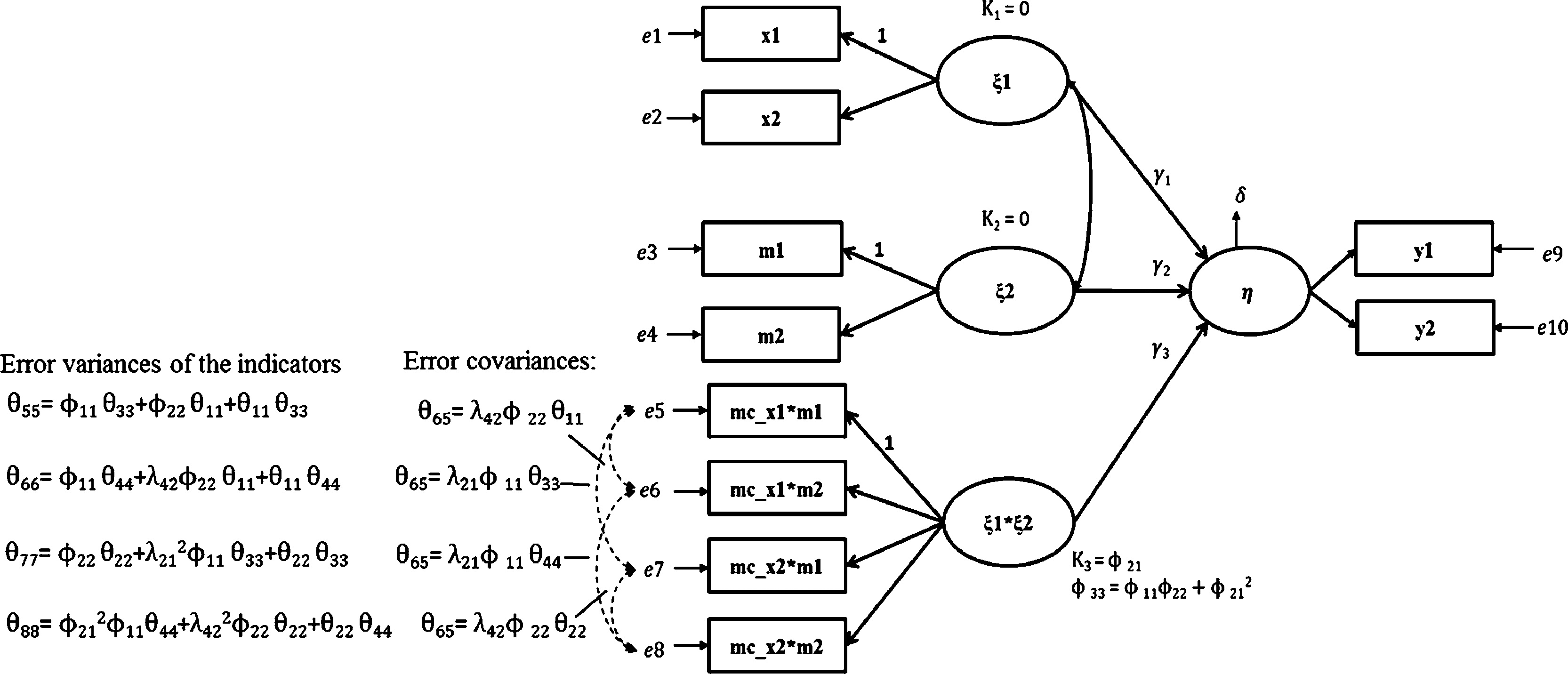
Past experience (PE) reduces risk of an unsatisfactory experience and is a good predictor of travellers’ intention to choose a destination (Gitelson & Crompton, 1984). The inclusion of PE in a model should increase the predictive capability of the original TPB (Kidwell & Jewell, 2007; Lam & Hsu, 2006; Smith et al., 2008). PE will likely influence people's deliberation and heuristic information processing with respect to SN and behavioural intention (Wood, Tam, & Witt, 2005). For instance, travellers with little travel experience may be more motivated to (re)visit a specific destination because they feel safe, want to investigate new aspects of the destination, or enrich the destination experience. In contrast, those with extensive travel experience may be less motivated to (re)visit a destination because based on their past experiences (and heuristics) there is less to uncover or experience at the destination. The inclusion of PE into TPB theory suggests SN will have a strong positive effect on behavioural intention when PE is low. Alternatively, when PE is high, SN may display a strong negative effect on behavioural intention. Therefore, the purpose of study one is to test the predicted moderating effects of PE on SN and Intention to Revisit (ITR). The proposed model and interaction (SN*PE) are displayed in Fig. 2.

Fig. 2.

Research model: Direct and Interaction Effects.

3.1. Sample

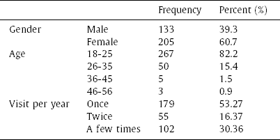
The study collected data through an intercept survey from 350 international tourists who visited Malaysia within the last year. After cleaning the data, the sample final size was 338; comprised of 205 females (60.7%) and 133 males, between 18 and 25 years of age (see Appendix D for additional detail). Twelve observations were discarded due to non-response and straight-lining (e.g., giving identical answers to items in a response scale) (Hair, Hult, Ringle, & Sarstedt, 2017; Kim, Dykema, Stevenson, Black, & Moberg, 2019).

3.2. Measurement

Each SN, PE, and ITR latent variable was measured with three indicators, adapted from previous studies (e.g., Huang & Hsu, 2009; Lam & Hsu, 2006; Mokhtaran, Fakharyan, Jalilvand, & Mohebi, 2015). The relative simplicity of the model adequately illustrates and demonstrate the three latent interaction analysis approaches. Regardless of the number of items used to measure the constructs in a model, the same procedures apply.

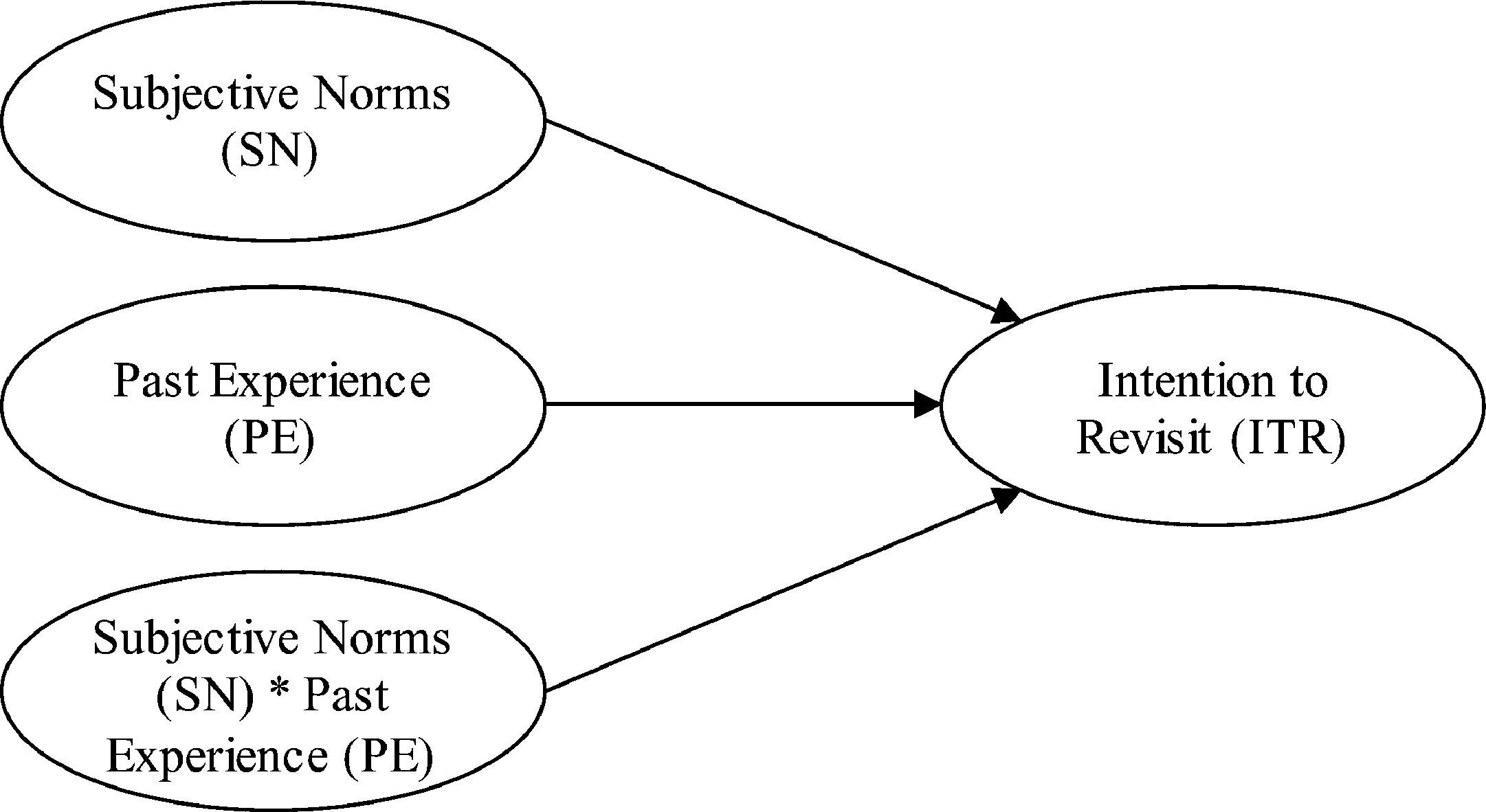
Table 1 reports acceptable result of reliability (both Cronbach's Alpha and Composite Reliability), construct convergent, and discriminant validity (Fornell & Larcker, 1981). In all cases the respondents’ level of agreement or disagreement was measured using 7-point Likert-type scales, anchored with 1 = Strongly Disagree to 7 = Strongly Agree.

Table 1
Item loadings, Cronbach's Alpha (CA), Composite Reliability (CR), Average Variance Explained (AVE), and Discriminant Validity.

Loading Cronbach's α CR AVE

Subjective Norm (SN)

The opinions of people who are important to me will affect my decision to revisit Malaysia. 0.830 0.791 0.797 0.563

I will have personal control over deciding to revisit Malaysia. 0.800

It is easy for me to decide Malaysia as my touring destination. 0.600

Past Experience (PE)

My overall evaluation on the past experience of visiting Malaysia is positive. 0.870 0.905 0.906 0.763

My overall evaluation on the past experience of visiting Malaysia is favorable’. 0.860

I am satisfied with my past experience of visiting Malaysia. 0.890

Intention to Revisit (ITR)

If I had to decide again I would choose visiting Malaysia again. 0.800 0.879 0.881 0.707

I will recommend Malaysia to friends and relatives. 0.900

I will speak highly of Malaysia to friends and relatives. 0.820

Fornell-Larcker Criterion* 1 2 3

1. Intention to Revisit 0.841

2. Past Experience 0.798 0.873

3. Subjective Norm 0.717 0.709 0.750

	Loading	Cronbach's α	CR	AVE
Subjective Norm (SN)
The opinions of people who are important to me will affect my decision to revisit Malaysia.	0.830	0.791	0.797	0.563
I will have personal control over deciding to revisit Malaysia.	0.800
It is easy for me to decide Malaysia as my touring destination.	0.600
Past Experience (PE)
My overall evaluation on the past experience of visiting Malaysia is positive.	0.870	0.905	0.906	0.763
My overall evaluation on the past experience of visiting Malaysia is favorable’.	0.860
I am satisfied with my past experience of visiting Malaysia.	0.890
Intention to Revisit (ITR)
If I had to decide again I would choose visiting Malaysia again.	0.800	0.879	0.881	0.707
I will recommend Malaysia to friends and relatives.	0.900
I will speak highly of Malaysia to friends and relatives.	0.820
Fornell-Larcker Criterion*	1	2	3
1. Intention to Revisit	0.841
2. Past Experience	0.798	0.873
3. Subjective Norm	0.717	0.709	0.750

Note: Loadings meet or exceed the minimum criteria (0.60), CA and CR exceed the minimum criteria (0.70), AVE exceed the minimum criteria (0.50) (Hair et al., 2010). Numbers on diagonal are the square root of the AVEs and off-diagonal numbers are inter-constructs correlations. All construct intercorrelations are less than the corresponding square root of the AVEs.

Subjective Norm (SN): The three item scale was adapted from Lam and Hsu (2006) to measure tourists SN.

Past Experience (PE): PE was measured using three items adapted from Huang and Hsu (2009).

Intention to Revisit (ITR): Mokhtaran et al.'s (2015) three item scale was used to measure tourists’ intention to revisit Malaysia.

3.3. Constrained, unconstrained and orthogonalized approaches

3.3.1. Constrained approach

The constrained approach was conducted based on the Algina and Moulder (2001) reformulation of the Jöreskog and Yang (1996) approach described earlier. Centred items were used to calculate the SN and PE product indicators. Since there were three items for both SN and PE, the latent interaction variable of SN_PE ended up with nine (three times three) product indicators. The item measuring intention was kept in its original scale. The SN and PE latent variables means were fixed to zero, and the mean of the SN_PE latent product term was constrained to be equal to the covariance of the latent variables SN and PE. In addition, the exogenous variables (SN, PE, and SN_PE) were allowed to correlate. The intercepts of the exogenous variable indicators were fixed to zero, but the intercept of the ITR items were estimated. Eighteen error covariances were estimated between product indicators which have a common component:

1.
the error of ‘MC_SN1_PE1’ covaried with the error of ‘MC_SN1_PE2’,
2.
the error of ‘MC_SN1_PE2’ covaried with the error of ‘MC_SN1_PE3’,
3.
the error of ‘MC_SN1_PE1’ covaried with the error of ‘MC_SN1_PE3’,
4.
the error of ‘MC_SN2_PE1’ covaried with the error of ‘MC_SN2_PE2’,
5.
the error of ‘MC_SN2_PE2’ covaried with the error of ‘MC_SN2_PE3’,
6.
the error of ‘MC_SN2_PE1’ covaried with the error of ‘MC_SN2_PE3’,
7.
the error of ‘MC_SN3_PE1’ covaried with the error of ‘MC_SN3_PE2’,
8.
the error of ‘MC_SN3_PE2’ covaried with the error of ‘MC_SN3_PE3’,
9.
the error of ‘MC_SN3_PE1’ covaried with the error of ‘MC_SN3_PE3’,
10.
the error of ‘MC_SN1_PE1’ covaried with the error of ‘MC_SN2_PE1’,
11.
the error of ‘MC_SN2_PE1’ covaried with the error of ‘MC_SN3_PE1’,
12.
the error of ‘MC_SN1_PE1’ covaried with the error of ‘MC_SN3_PE1’,
13.
the error of ‘MC_SN1_PE2’ covaried with the error of ‘MC_SN2_PE2’,
14.
the error of ‘MC_SN2_PE2’ covaried with the error of ‘MC_SN3_PE2’,
15.
the error of ‘MC_SN1_PE2’ covaried with the error of ‘MC_SN3_PE2’
16.
the error of ‘MC_SN1_PE3’ covaried with the error of ‘MC_SN2_PE3’,
17.
the error of ‘MC_SN2_PE3’ covaried with the error of ‘MC_SN3_PE3’,
18.
the error of ‘MC_SN1_PE3’ covaried with the error of ‘MC_SN3_PE3’,

Lastly, the non-covariances between error terms were fixed to zero because these product indicators had no common component (Fig. 3).

Fig. 3.
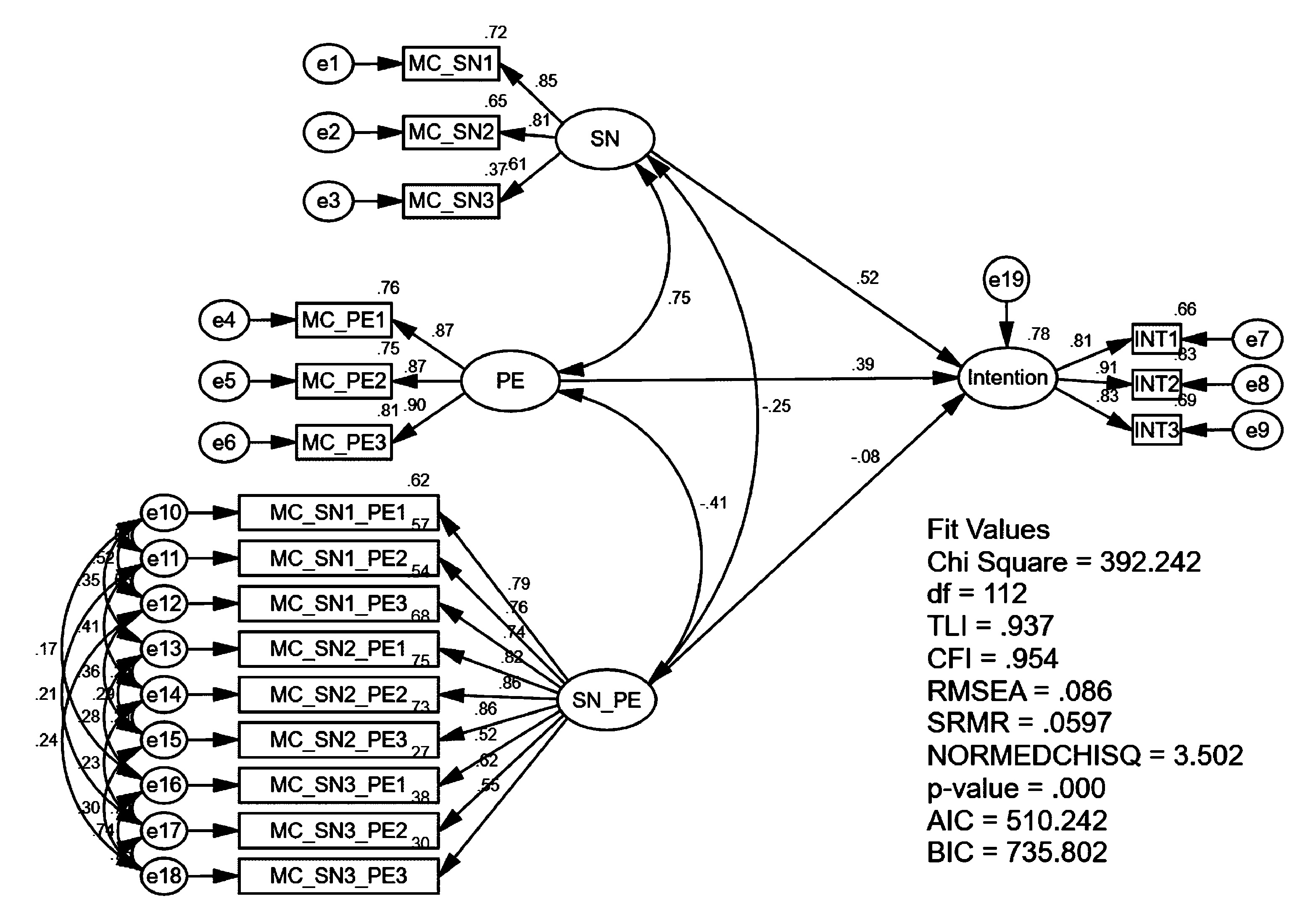
A latent variable interaction using constrained approach.
3.3.2. Unconstrained approach

For the unconstrained approach, the double-mean-centring strategy was used in the unconstrained approach (Lin et al., 2010)(Fig. 4). Since both first-order effects, SN and PE are measured with three indicators each, the latent interaction variable SN_PE consisted of nine (three times three) product indicators. Guided by Lin et al. (2010), the indicators of both SN and PE were first mean-centred before calculating the product indicators. Then, the mean-centred of SN and PE were multiplied together to form the nine product indicators. These nine product indicators of SN_PE were mean-centred again before calculating the latent interaction result. By using the double-mean-centring strategy, the researcher does not need to constrain the mean of the interaction latent factor equal to the covariance between the two main latent factors. Moreover, the items measuring Intention (ITR) were not mean-centred. In addition, the exogenous variables (SN, PE, and SN_PE) were allowed to correlate. Eighteen error covariances were estimated between product indicators which have a common component:

1.
the error of ‘DMC_SN1_PE1’ covaried with the error of ‘DMC_SN1_PE2’,
2.
the error of ‘DMC_SN1_PE2’ covaried with the error of ‘DMC_SN1_PE3’,
3.
the error of ‘DMC_SN1_PE1’ covaried with the error of ‘DMC_SN1_PE3’,
4.
the error of ‘DMC_SN2_PE1’ covaried with the error of ‘DMC_SN2_PE2’,
5.
the error of ‘DMC_SN2_PE2’ covaried with the error of ‘DMC_SN2_PE3’,
6.
the error of ‘DMC_SN2_PE1’ covaried with the error of ‘DMC_SN2_PE3’,
7.
the error of ‘DMC_SN3_PE1’ covaried with the error of ‘DMC_SN3_PE2’,
8.
the error of ‘DMC_SN3_PE2’ covaried with the error of ‘DMC_SN3_PE3’,
9.
the error of ‘DMC_SN3_PE1’ covaried with the error of ‘DMC_SN3_PE3’,
10.
the error of ‘DMC_SN1_PE1’ covaried with the error of ‘DMC_SN2_PE1’,
11.
the error of ‘DMC_SN2_PE1’ covaried with the error of ‘DMC_SN3_PE1’,
12.
the error of ‘DMC_SN1_PE1’ covaried with the error of ‘DMC_SN3_PE1’,
13.
the error of ‘DMC_SN1_PE2’ covaried with the error of ‘DMC_SN2_PE2’,
14.
the error of ‘DMC_SN2_PE2’ covaried with the error of ‘DMC_SN3_PE2’,
15.
the error of ‘DMC_SN1_PE2’ covaried with the error of ‘DMC_SN3_PE2’
16.
the error of ‘DMC_SN1_PE3’ covaried with the error of ‘DMC_SN2_PE3’,
17.
the error of ‘DMC_SN2_PE3’ covaried with the error of ‘DMC_SN3_PE3’,
18.
the error of ‘DMC_SN1_PE3’ covaried with the error of ‘DMC_SN3_PE3’,

Fig. 4.
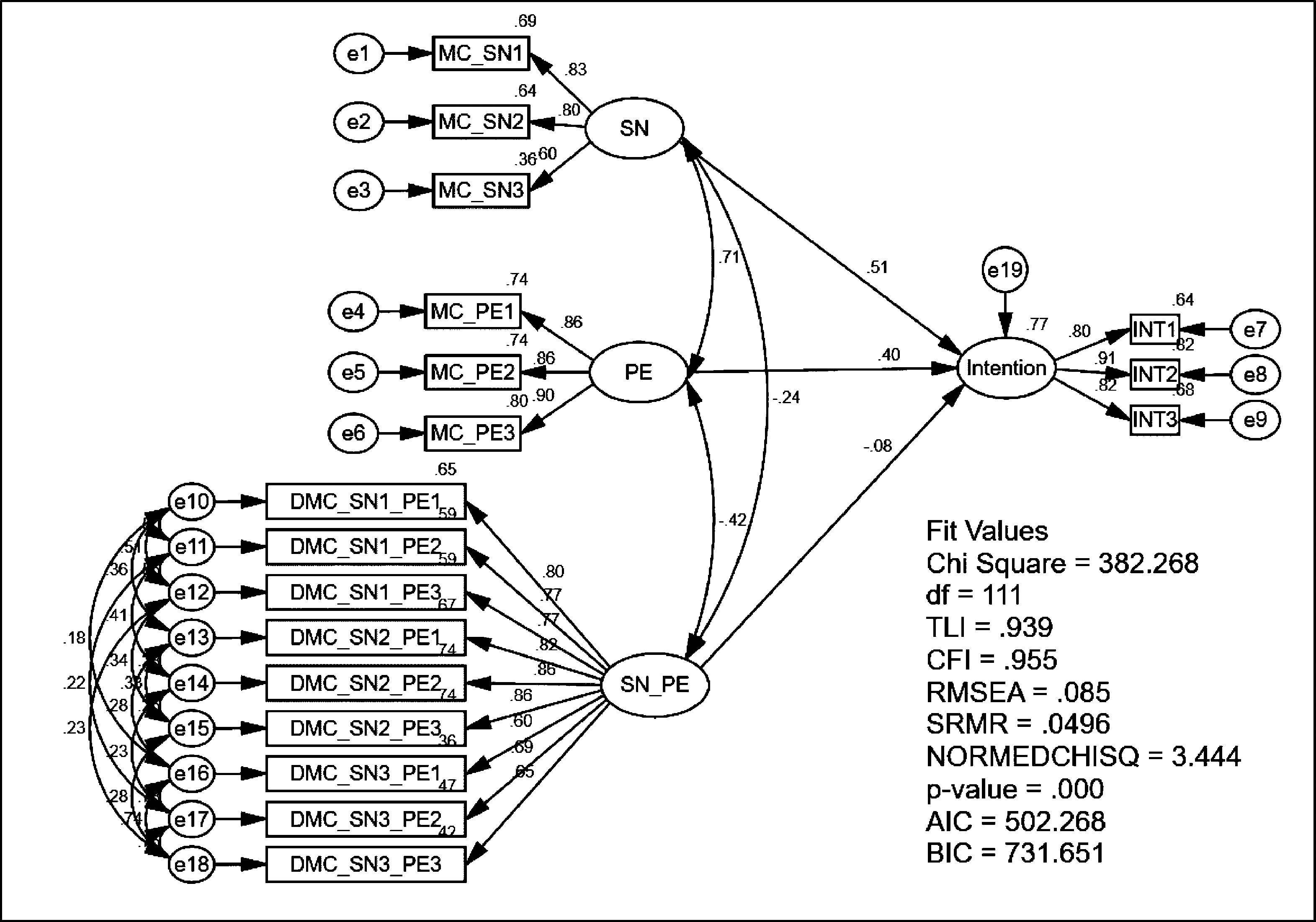
A latent variable interaction using unconstrained approach.

Lastly, the non-covariances between error terms were fixed to zero because these product indicators had no common component (Fig. 4).
3.3.3. Orthogonalized approach

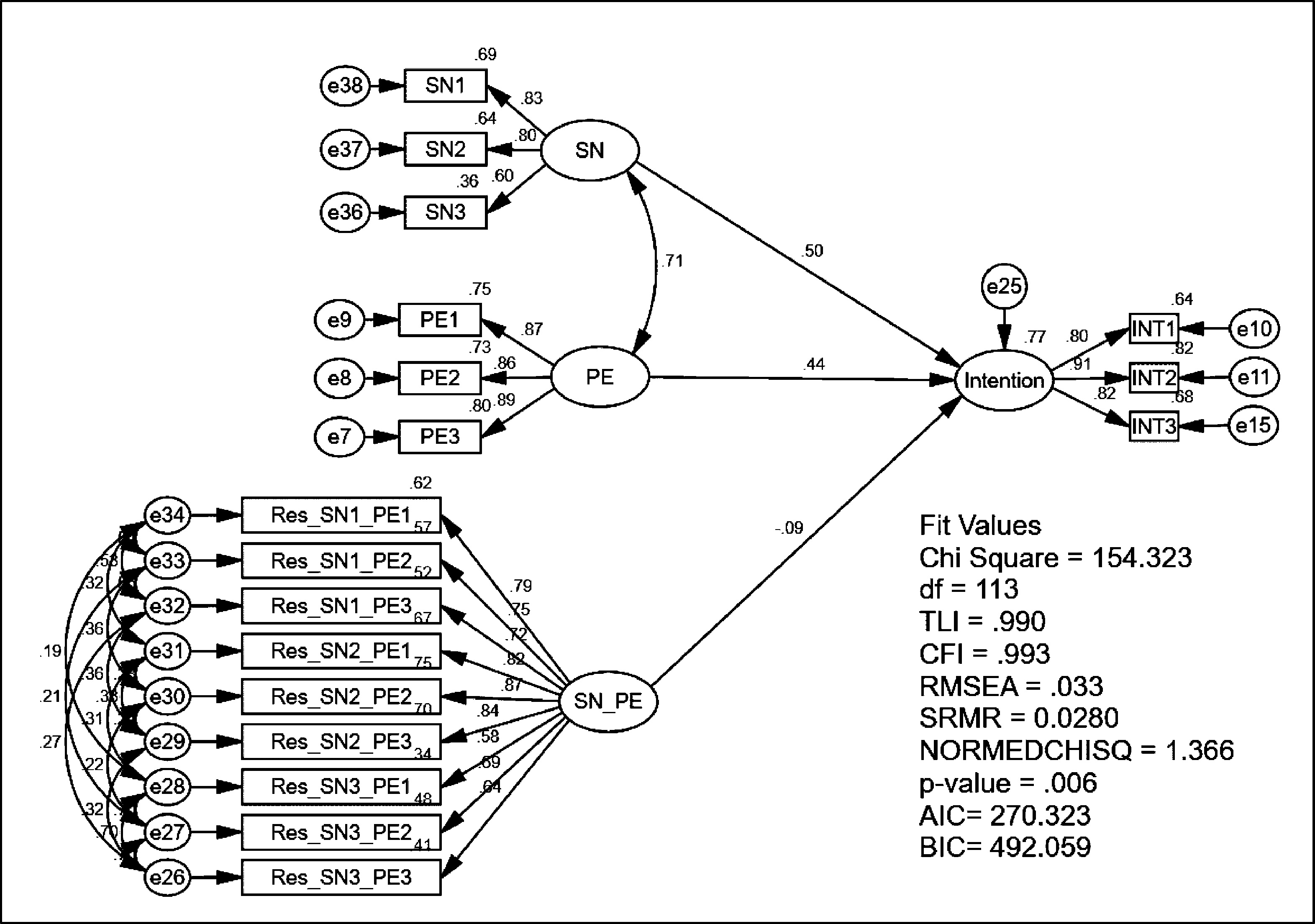
The orthogonalized approach was computed in two steps (Little et al., 2006). In step 1 the uncentered SN indicator was multiplied with the uncentered PE indicator. This resulted in nine indicators for the interaction variable (SN_PE): SN1*PE1, SN1*PE2, SN1*PE3, SN2*PE1, SN2*PE2, SN2*PE3, SN3*PE1, SN3*PE2, and SN3*PE3 (see Fig. 5).

Fig. 5.

A latent variable interaction using orthogonalized approach.

Fig. 6.

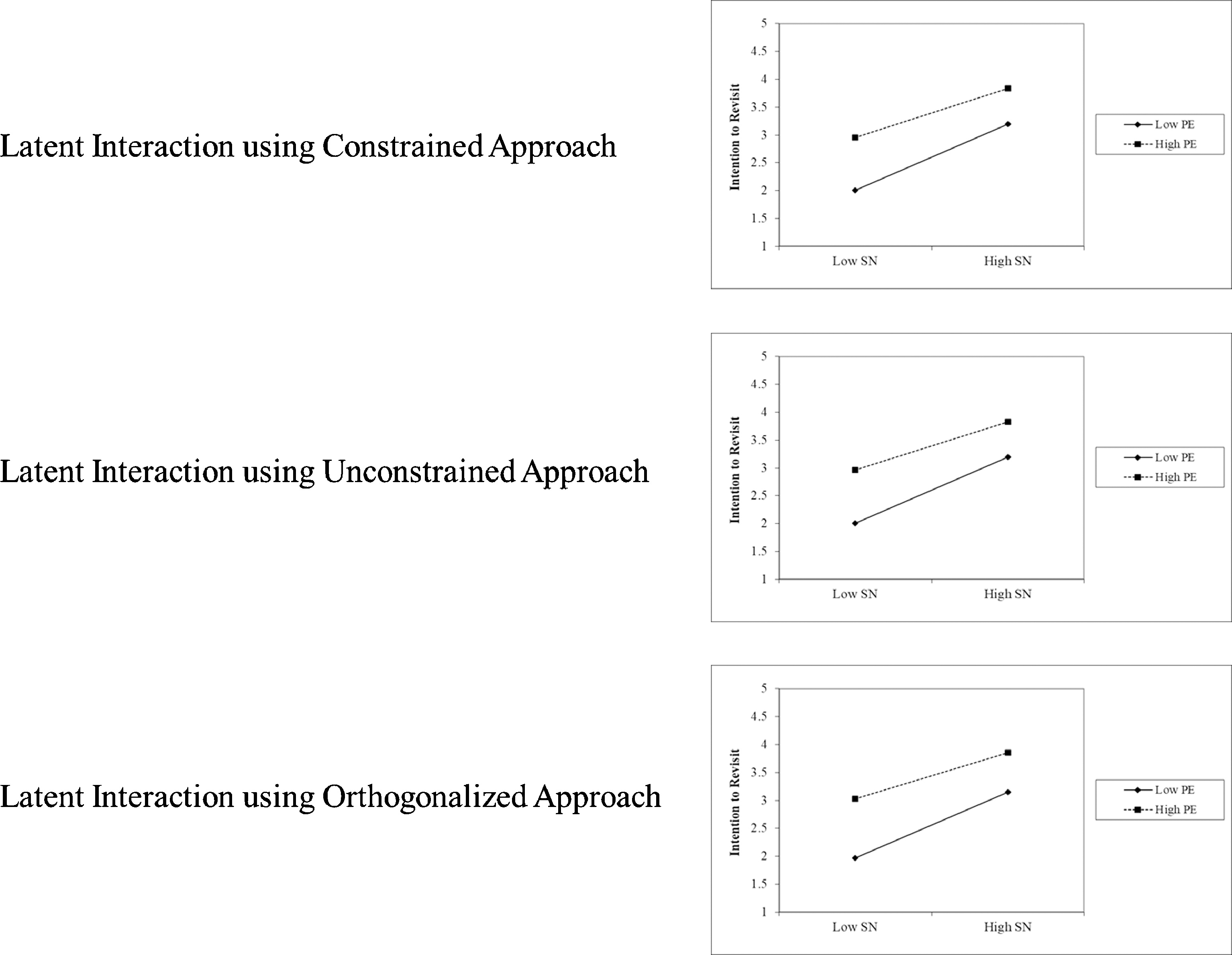
The nature of interaction plot for all three approaches.

Nine new residual-based indicators were created from the residuals of the regression of all exogenous indicators (e.g., SN1…PE3) on each of the nine new interactive variable indicators¹. Computing the regression for all nine interactive indicator variables (e.g., SN1*PE1, SN1*PE2,…, SN3*PE3) produces nine regression residuals (Res_ SN1PE1, Res_ SN1PE2,… Res_ SN3PE3). The nine regression residuals were used as measures of the latent variable interaction.

Detailed instructions how to save residuals using SPSS ver 25 can be found in Appendix C.

In the second step, the latent interaction model was specified; three SN items as indicators of the SN variable, three PE items as indicators of the PE variable, and nine regression residuals as indicators of the latent SN_PE variable interaction. For each latent variable (SN, PE, and the latent variable interaction SN_PE), one factor loading was fixed in order to provide a scale for the respective latent variables (i.e., fix the factor loading of the first indicator to 1). Finally, eighteen error covariances between nine pairs of the SN_PE residual product indicators were specified: 1.

error of ‘Res_SN1_PE1’ covaried with the error of ‘Res_SN1_PE2’,

error of ‘Res_SN1_PE2’ covaried with the error of ‘Res_SN1_PE3’,

error of ‘Res_SN1_PE1’ covaried with the error of ‘Res_SN1_PE3’,

error of ‘Res_SN2_PE1’ covaried with the error of ‘Res_SN2_PE2’,

error of ‘Res_SN2_PE2’ covaried with the error of ‘Res_SN2_PE3’,

error of ‘Res_SN2_PE1’ covaried with the error of ‘Res_SN2_PE3’,

error of ‘Res_SN3_PE1’ covaried with the error of ‘Res_SN3_PE2’,

error of ‘Res_SN3_PE2’ covaried with the error of ‘Res_SN3_PE3’,

error of ‘Res_SN3_PE1’ covaried with the error of ‘Res_SN3_PE3’,

10.

error of ‘Res_SN1_PE1’ covaried with the error of ‘Res_SN2_PE1’,

11.

error of ‘Res_SN2_PE1’ covaried with the error of ‘Res_SN3_PE1’,

12.

error of ‘Res_SN1_PE1’ covaried with the error of ‘Res_SN3_PE1’,

13.

error of ‘Res_SN1_PE2’ covaried with the error of ‘Res_SN2_PE2’,

14.

error of ‘Res_SN2_PE2’ covaried with the error of ‘Res_SN3_PE2’,

15.

error of ‘Res_SN1_PE2’ covaried with the error of ‘Res_SN3_PE2’,

16.

error of ‘Res_SN1_PE3’ covaried with the error of ‘Res_SN2_PE3’,

17.

error of ‘Res_SN2_PE3’ covaried with the error of ‘Res_SN3_PE3’,

18.

error of ‘Res_SN1_PE3’ covaried with the error of ‘Res_SN3_PE3’,

This procedure freed the error correlation of the residual product indicators from the multiplication of the same first-order effect items (SN and PE), thereby ensuring the residual product indicators had no common component with the first-order effect items. By covarying the residuals (see 1-18), the analysis ensures that the indicators of the interaction term do not share any variance with the indicators of the exogenous construct and the moderator, that is, the interaction term is orthogonal to the other two constructs, precluding any collinearity issues among the constructs.

4. Data analysis

Analyses were conducted using AMOS 25.0 Bootstrap Maximum Likelihood (BML) since the latent product variable is not normally distributed (Arbuckle, 2017). The BML procedure produces appropriate standard errors adjusting for lack of multivariate normality (Byrne, 2016; Hoyle, 2012). As recommended by Hair et al. (2010) 5,000 bootstrap subsamples were performed.

4.1. Descriptive statistics

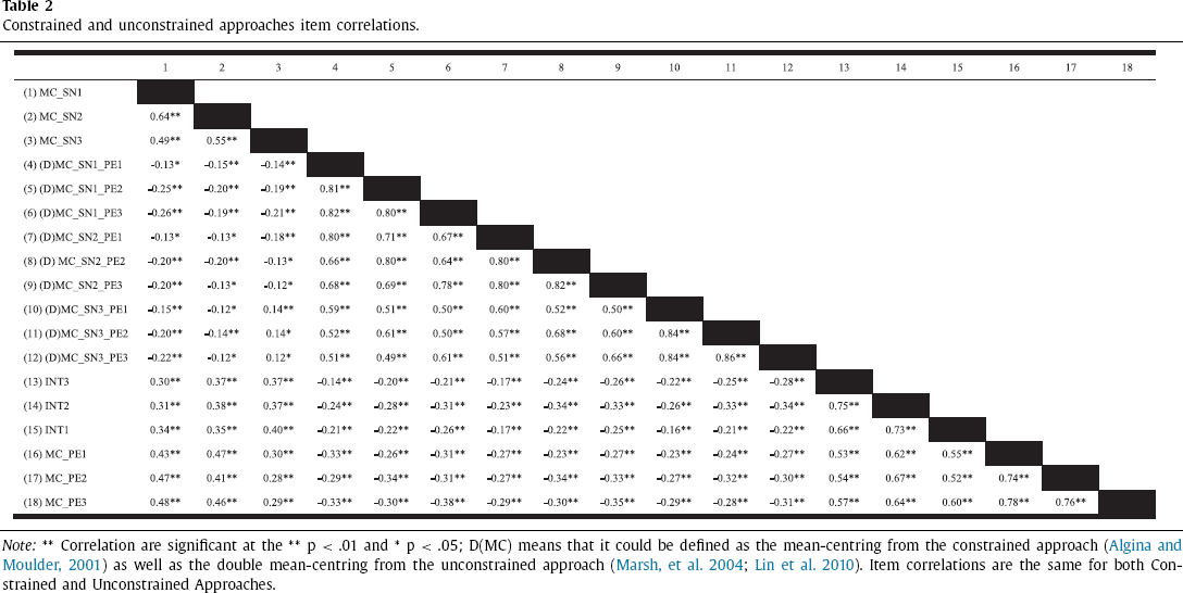
Although the first-order effect indicators (SN and PE) correlate significantly with the latent product indicator terms under the Constrained Approach and Unconstrained Approach (see Table 2), due to mean-centring and double mean-centring, multicollinearity is not an issue (Algina & Moulder, 2001; Lin et al., 2010). The mean-centred indicators for SN and PE and the latent product interaction are shown in Table 3. The latent product indicator data exhibits positive skewness and kurtosis, while SN, PE, and INT (ITR) indicator data exhibit slight skewness, but are within acceptable limits for analysis (Lei & Lomax, 2005)².

2
The significance correlations occurring in the constrained and unconstrained approaches between the first-order effect indicators and the product indicators result partly from the severe level of nonnormality of the predictor variables in our study. Nonnormality is a typical problem in a model that includes interaction terms and is especially evident when Likert scales are used (Flora & Curran, 2004)

Table 2

Constrained and unconstrained approaches item correlations.

Table 3

Constrained and unconstrained approaches - means, standard deviations, skewness, and kurtosis.

	M	SD	Skew	Kurtosis
INT1	5.46	1.18	-0.94	1.18
INT2	5.64	1.11	-1.16	1.58
INT3	5.46	1.11	-0.79	0.81
MC_SN1	0.00	1.12	-1.07	1.43
MC_SN2	0.00	1.26	-0.93	0.49
MC_SN3	0.00	1.26	-1.09	1.32
MC_PE1	0.00	0.97	-0.86	1.12
MC_PE2	0.00	0.94	-0.85	1.28
MC_PE3	0.00	1.03	-1.08	1.55
(D)MC_SN1_PE1	0.57	1.31	3.16	24.57
(D)MC_SN1_PE2	0.60	1.42	3.72	21.64
(D)MC_SN1_PE3	0.67	1.49	3.53	19.38
(D)MC_SN2_PE1	0.57	1.40	3.04	18.13
(D)MC_SN2_PE2	0.60	1.62	3.26	18.28
(D)MC_SN2_PE3	0.60	1.62	2.93	16.69
(D)MC_SN3_PE1	0.37	1.37	1.61	18.27
(D)MC_SN3_PE2	0.32	1.50	1.54	15.78
(D)MC_SN3_PE3	0.38	1.58	1.50	13.38

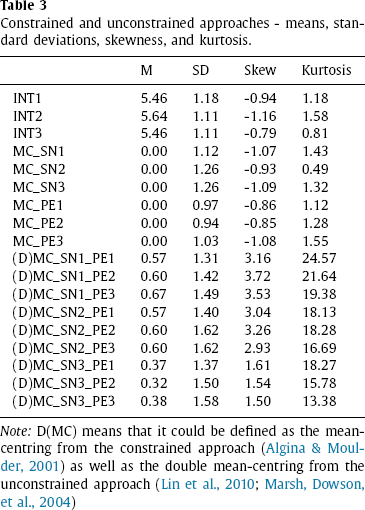
Note: D(MC) means that it could be defined as the mean-centring from the constrained approach (Algina & Moulder, 2001) as well as the double mean-centring from the unconstrained approach (Lin et al., 2010; Marsh, Dowson, et al., 2004)

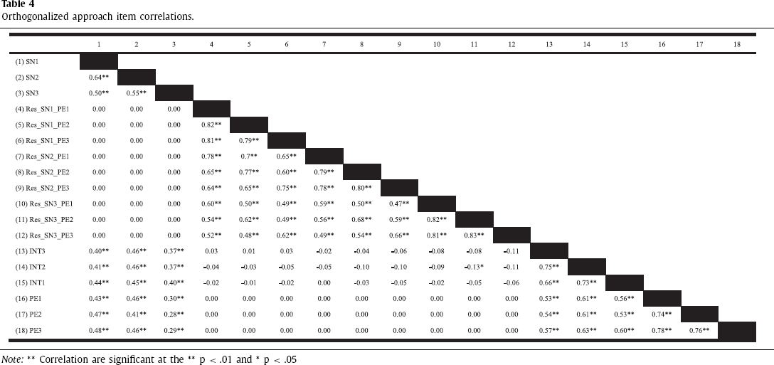
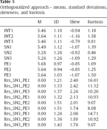
As expected from the Orthogonalized Approach using residual centring (refer to Table 4), the first-order effect indicators (SN and PE) show zero correlation with those of the latent product indicator terms (Little et al., 2006; Steinmetz et al., 2011). Using residuals as indicators for the latent product interaction items, results in residuals being purged from the common variance between the SN and PE first-order effect indicators and the latent product indicators. Table 5 reports the means, standard deviations, skewness, and kurtosis of the residual centring model approach. The latent product indicator data exhibits positive skewness and kurtosis, while SN, PE, and INT (ITR) indicator data exhibit slight skewness but are within acceptable limits.

Table 4

Orthogonalized approach item correlations.

Table 5

Orthogonalized approach - means, standard deviations, skewness, and kurtosis.

	M	SD	Skew	Kurtosis
INT1	5.46	1.18	-0.94	1.18
INT2	5.64	1.11	-1.16	1.58
INT3	5.46	1.11	-0.79	0.81
SN1	5.49	1.12	-1.07	1.39
SN2	5.28	1.26	-0.92	0.46
SN3	5.26	1.26	-1.09	1.29
PE1	5.68	0.97	-0.85	1.09
PE2	5.64	0.94	-0.85	1.25
PE3	5.64	1.03	-1.07	1.50
Res_SN1_PE1	0.00	1.21	2.40	16.01
Res_SN1_PE2	0.00	1.33	2.42	11.32
Res_SN1_PE3	0.00	1.37	2.26	10.20
Res_SN2_PE1	0.00	1.32	2.13	10.93
Res_SN2_PE2	0.00	1.51	2.01	9.07
Res_SN2_PE3	0.00	1.51	1.74	8.08
Res_SN3_PE1	0.00	1.26	2.06	14.71
Res_SN3_PE2	0.00	1.36	1.88	10.92
Res_SN3_PE3	0.00	1.43	1.76	9.07

4.2. Findings from the three approaches

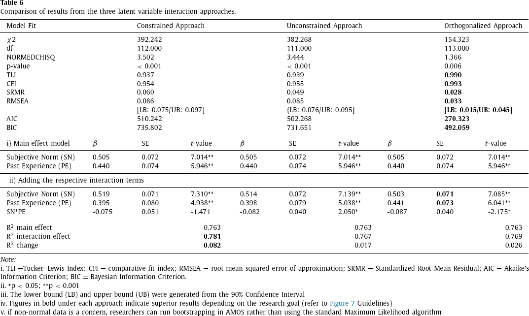
Reviewing the Goodness of Fit (GoF) criteria (see Table 6), to help identify which model best fits the data, the orthogonalized residual centring approach appears to outperform the constrained and unconstrained approach across the GoF dimensions; NORMEDCHISQ = 1.366 vs 3.444 vs 3.502, TLI = 0.990 vs 0.939 vs 0.937, CFI = 0.993 vs 0.955 vs 0.954, RMSEA = 0.033 vs 0.085 vs 0.086, SRMR = 0.028 vs 0.049 vs 0.060 (Bagozzi & Yi, 2012).

The Akaike's Information Criterion (AIC) and Bayesian Information Criterion (BIC) are information indexes used to determine which model best approximates the data (Vrieze, 2012). When comparing non-nested models, smaller values indicate better models both in terms of model fit, model parsimony and minimizing information loss.

Considering AIC and BIC, the orthogonalized approach (AIC = 270.32, BIC = 492.06) is preferable to the unconstrained approach (AIC = 502.268, BIC = 731.651) and constrained approach (AIC = 510.24, BIC = 735.80). All three approaches result in comparable latent parameter first-order estimates (or main effect model), indicating that ITR is positively and significantly influenced by SN and PE. The interaction effect was negative in all three cases. The orthogonalized approach revealed a better significant SN*PE interaction effect (β = -0.087, t = -2.175, p < 0.05) than the unconstrained approach (β = -0.082, t = -2.050, p < 0.05), while the constrained approach reported a non-significant SN*PE interaction effect (β = -0.075, t = -1.471, p > 0.05), refer to the lower half of Table 6.

Table 6
Comparison of results from the three latent variable interaction approaches.

Model Fit Constrained Approach Unconstrained Approach Orthogonalized Approach

χ2 392.242 382.268 154.323

df 112.000 111.000 113.000

NORMEDCHISQ 3.502 3.444 1.366

p-value < 0.001 < 0.001 0.006

TLI 0.937 0.939 0.990

CFI 0.954 0.955 0.993

SRMR 0.060 0.049 0.028

RMSEA 0.086 0.085 0.033

[LB: 0.075/UB: 0.097] {LB: 0.076/UB: 0.095] [LB: 0.015/UB: 0.045]

AIC 510.242 502.268 270.323

BIC 735.802 731.651 492.059

i) Main effect model β SE t-value β SE t-value β SE t-value

Subjective Norm (SN) 0.505 0.072 7.014 0.505 0.072 7.014 0.505 0.072 7.014

Past Experience (PE) 0.440 0.074 5.946 0.440 0.074 5.946 0.440 0.074 5.946

ii) Adding the respective interaction terms

Subjective Norm (SN) 0.519 0.071 7.310 0.514 0.072 7.139 0.503 0.071 7.085

Past Experience (PE) 0.395 0.080 4.938 0.398 0.079 5.038 0.441 0.073 6.041

SNPE -0.075 0.051 -1.471 -0.082 0.040 2.050 -0.087 0.040 -2.175*

R² main effect 0.763 0.763 0.763

R² interaction effect 0.781 0.767 0.769

R² change 0.082 0.017 0.026

Model Fit	Constrained Approach	Unconstrained Approach	Orthogonalized Approach
χ2	392.242	382.268	154.323
df	112.000	111.000	113.000
NORMEDCHISQ	3.502	3.444	1.366
p-value	< 0.001	< 0.001	0.006
TLI	0.937	0.939	0.990
CFI	0.954	0.955	0.993
SRMR	0.060	0.049	0.028
RMSEA	0.086	0.085	0.033
	[LB: 0.075/UB: 0.097]	{LB: 0.076/UB: 0.095]	[LB: 0.015/UB: 0.045]
AIC	510.242	502.268	270.323
BIC	735.802	731.651	492.059

Note: i. TLI =Tucker–Lewis Index; CFI = comparative fit index; RMSEA = root mean squared error of approximation; SRMR = Standardized Root Mean Residual; AIC = Akaike's Information Criterion; BIC = Bayesian Information Criterion.

ii. *p < 0.05; **p < 0.001

iii. The lower bound (LB) and upper bound (UB) were generated from the 90% Confidence Interval

iv. Figures in bold under each approach indicate superior results depending on the research goal (refer to Figure 7 Guidelines)

v. if non-normal data is a concern, researchers can run bootstrapping in AMOS rather than using the standard Maximum Likelihood algorithm

The incremental R² change between the main effect results and adding the interaction effect for the constrained approach R² was 0.082; the inclusion of the interaction term increased the explanation power by 8.2%, representing a small effect, f ² = .089 (Carte & Russell, 2003; Cohen, 1988). For the orthogonalized approach, the incremental R² was 0.026 indicating an increase in explanation power by 2.6%, which also signifies a small effect, f ² = .027. On the other hand, the unconstrained approach exhibits the smallest incremental R² value of .017 indicating an increase in explanatory power by 1.7%, representing a small effect, f ² = .017. In this study, the small incremental interaction effect from both the unconstrained and orthogonalized approaches can be interpreted as meaningful since the resulting beta change is significant (Chin, Marcolin, & Newsted, 2003).

There are several interesting findings that can be observed from the comparison of approaches. The results indicate that the constrained approach has slightly better explanatory power compared to both the unconstrained and orthogonalized approaches. One of the reasons is that the constrained interaction contains both the unique and shared variance that fully represents the interaction effect. In contrast, the variance of both the unconstrained orthogonalized interaction term contains only the unique variance (from double mean-centring and residual value for interaction), the unique variance of each indicator is counted only once in the variance of the latent interaction effect (the multiplying of pair indicators) while shared variance is counted three times — once within the variance term of the latent interaction effect and twice among the covariances. Therefore, the constrained approach maximizes the explained variance of the endogenous latent variable compared to the unconstrained and orthogonalized approaches because the indicators of the interaction term of the indicators do share variance with indicators of the exogenous latent variable (SN) and the moderator (PE).

The constrained approach exhibits the highest explanatory power of interaction effects. This effect comes at a cost, namely the downward biased estimation of the single or main effects. Similarly, such result also occurs on the unconstrained approach. Table 6 indicates that the path coefficient estimates (β) without the interaction term in the two models are identical. The result of the interaction term was consistent with Little et al. (2006) finding, who found that the orthogonalized approach prevents changes in the standardized beta coefficient result of independent variable when running the interaction. Therefore, correlated error structure provides unbiased estimates, which indirectly increases the interpretability of the overall results of the moderator analysis. The characteristics of the orthogonalized approach facilitates interpretation of the moderating effect strength compared to both constrained and unconstrained approach.

Fig. 5 illustrates the nature of the SN*PE interaction for all three approaches - constrained, unconstrained and orthogonal approach. Both the unconstrained and orthogonal approaches indicate a statistically significant effect of past experience (PE) on intention to revisit (ITR) dependent on subjective norm (SN) (see Table 6).

Of particular interest is the finding that the constrained (mean-centred) approach produces high kurtosis (platykurtic) in the interaction latent variable (SN*PE) (Table 3), which also manifests in larger standard error (SE) (cf. Fan & Wang, 1998; Finch, West, & MacKinnon, 1997). The orthogonal approach does not produce the same level of kurtosis in the interaction latent variable (SN*PE) (Table 5), which manifests in smaller standard error. This difference in standard error produces significantly different results. On the other hand, the result produced from the unconstrained approach was exceptional because the double mean-centring helps to reduce the standard error during the estimation of the structural model. This result implies that the constrained (mean-centred) approach may provide a more conservative biased result compared to both the unconstrained and orthogonal approach. Contrary to the Lei and Lomax (2005) findings, the results from our current study demonstrate the potential effect of SE bias on the interaction results depending on the latent interaction modelling approach.

Although High PE indicates an overall stronger propensity to revisit, the line labelled Low PE has a steeper gradient. This indicates that SN has a stronger effect on ITR when PE is lower. This interaction indicates that travellers with little past experience may be more motivated to (re)visit a destination based on SN in order to enhance their destination experiences (Wood et al., 2005).

The results indicate that both the unconstrained and orthogonalized approaches result in nearly identical parameter estimates to the constrained approach. However, only the constrained approach interaction effect is not significant, the reduced standard error from the unconstrained and orthogonalized approaches detect a significant interaction effect between SN and PE as expected by the TPB model (Anastasopoulos, 1992; Kidwell & Jewell, 2007; Smith et al., 2008).

5. Discussion

The estimation of interaction effects between latent variables with CB-SEM requires sophisticated analysis methods when the latent variables are measured with multiple indicators, since a number of complex constraints should be imposed on the model. Due to these constraint requirements few researchers include an empirical test of latent variables interaction effect used CB-SEM (Grissemann & Stokburger-Sauer, 2012; Yeh & Ku, 2017). This is unfortunate since CB-SEM methods control for measurement error and possess more power than conventional regression analysis to detect interaction effects.

The objectives of this paper are threefold. First, the paper outlines the implications of the constrained, unconstrained, and orthogonalized approaches to represent latent variable interactions in CB-SEM (e.g., AMOS). Second, using TPB as a foundation the study analyses a theoretically postulated interaction effect between SN and PE in the marketing domain and highlights several merits of the constrained, unconstrained, and orthogonalized approaches. Third, the paper provides guidelines for creating CB-SEM latent interaction terms for analysis.

The latent interaction effect for both the unconstrained and orthogonalized approach perform similarly with respect to the path coefficient estimates as well as effect size (Little et al., 2006; Steinmetz et al., 2011). The interaction between SN and PE hypothesized by TPB were similar using both approaches, however only the results from the unconstrained and orthogonalized approach were statistically significant. The study found both the constrained and unconstrained approaches generated better explanatory power than the orthogonalized approach due to the effect of both unique and shared variance from the observed covariation pattern among all possible indicators of the interaction.

The analysis demonstrated that the orthogonalized approach results in better model fit, with intercorrelations among the indicators reduced to zero and no multicollinearity concerns. Another consequence of the orthogonalized approach is that the path coefficient estimates in the model without the interaction term are identical to those with the interaction term. This characteristic greatly facilitates the interpretation of the moderating effects’ strength compared with both the constrained and the unconstrained approaches.

Scholars should consider either the unconstrained or the orthogonalized approach to better identify, analyse and interpret latent interaction effects. First and foremost, information loss is substantially reduced, both latent variable interaction approaches are derived from the observed covariation pattern among all possible indicators of the interaction. Second, there are no complicated constraints that need to be calculated for either approach. Third, no recalculations of parameters are required for either approach. Finally, both procedures can be performed using standard structural model software (e.g., AMOS, LISREL, SEPATH, EQS, Ωnyx, lavvan, and Mplus).

5.1. Recommendation

To aid researchers to achieve satisfactory results when assessing the latent interaction effects and provide guidelines for the use of the three approaches, a step-wise process of assessing the latent interaction effect in CB-SEM is presented in Fig. 7.

Fig. 7.

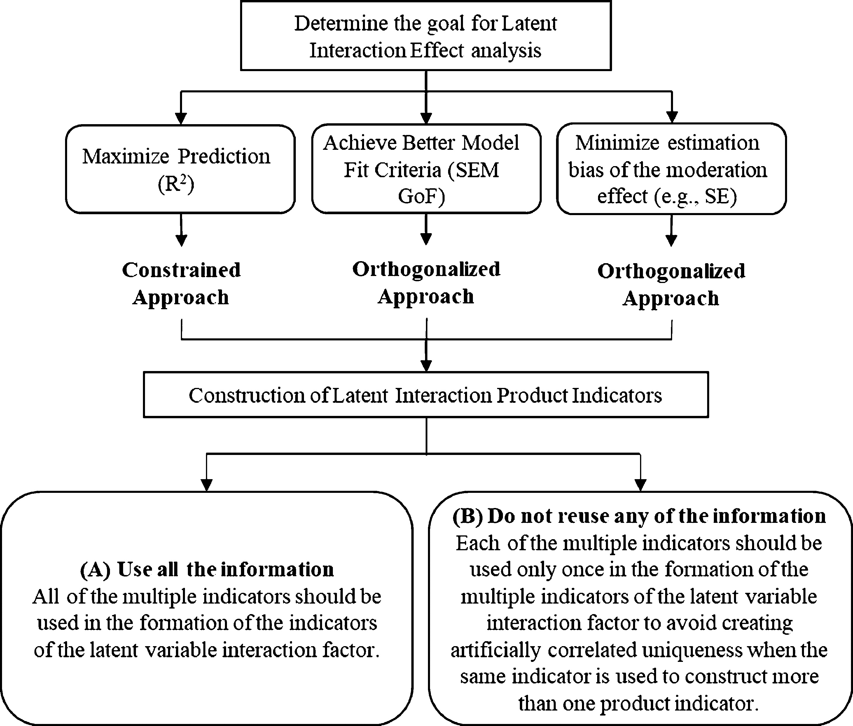
Guidelines for Creating the Latent Interaction Term in CB-SEM. Note: (A) is suitable to used when the number of matched-pair strategy to constructing interaction indicators is small (9 and below or use when sample size is large); (B) is suitable to used when the number of matched-pair strategy to constructing interaction indicators is large (9 and above or use when sample size is small) ( Marsh et al., 2004 ; 2006 ).

Firstly, researchers must consider the goal of the analysis for the latent interaction effects in CB-SEM. Goal analysis can be divided into three aspects: 1) Maximize prediction, 2) achieve better model fit, and 3) minimize estimate bias of the moderating effect. If satisfactory model fit and multicollinearity are not an issue the unconstrained approach is recommended. However, if the researcher faces both issues (unsatisfactory model fit and collinearity), the orthogonalized approach is recommended as it produces better model fit results and reduces collinearity issues. Importantly, our comparison study of the three approaches does not encourage researchers to estimate the latent interaction effect using the constrained approach because the constrained approach does not produce satisfactory path coefficient results or model fit.

Secondly, researchers should consider the construction of latent interaction indicators within the model. There are two key recommendations (Marsh & Craven, 2006; Marsh, Hau, et al., 2004): 1)

use all the available information. All first-order multiple indicators should be used in the formation of the latent variable interaction indicators. This is especially important when the number of constructed latent interaction indicators is small (9 and below), and/or when the sample size is large (n ≥ 200), and

do not reuse information (multiple indicators should be used only once), especially when the number of constructed latent interaction indicators is large (9 and above) or when sample size is small (n ≤ 200).

In the construction of the product indicators for the latent interaction variable (e.g., ξ1*ξ2 items), some situations may have natural matching that should be used to form product indicators (e.g., when ξ1 and ξ2 items have parallel wording) or more generally, when the two first-order effect factors, ξ1 and ξ2, have the same number of indicators. In other circumstances it may be better to match the ξ1 and ξ2 indicators in terms of the highest loadings of the indicators; the best item from the first factor with the best item from the second factor, etc. (Marsh, Hau, et al., 2004; Saris, Batista-Foguet, & Coenders, 2007).

When the number of indicators differs for the two first-order effect factors, then a simple matching strategy does not work. For example, when there are five indicators for the first factor and ten for the second factor. One approach is to use the ten items from the second factor to form five (item-pair) parcels by taking the average of the first two items to form the first item parcel, the average of the second two items to form the second parcel, and so forth. Consequently, the first factor would be defined in terms of five (single-indicator) indicators, the second factor would be defined by five (item-pair parcel) indicators, and the latent interaction factor would be defined in terms of five matched-product indicators. Little, Cunningham, Shahar, and Widaman (2002) provide additional detail and explanation regarding the parcelling procedure.

For exploratory research the orthogonalized approach is recommended since it is less likely to have factor score indeterminacy issues, and more likely to produce smaller SE (i.e., less conservative) results.

5.2. Limitations

As with most research this study has a number of limitations. Although three indicators per latent variable, and three single indicators for the intention to revisit, is not necessarily representative, the small number of items per variable enables a clear and understandable presentation of the two methodology approaches. Future research should estimate and compare the constrained, unconstrained, and orthogonalization approaches using more than three indicators per construct.

This study is limited to the use of a 7-point Likert scale in assessing the latent interaction effect in CB-SEM. To provide a better comparison test between constrained, unconstrained and orthogonalized approaches, future research could compare the result of Likert-type scales with 5-point, 7-point or 10-point format. Using different scale formats (anchors) may affect the data in terms of assessing the latent interaction effect when looking into the results of path-coefficient, explanatory power, and model fit.

The empirical example in this study relies on using all multiple indicators in the construction of the latent interaction variable. This limits the generalizability under a matched-pair strategy condition when constructing interaction indicators with a large number of indicators. The recommendation for future researchers is to implement the matched pair strategies when constructing the indicators to identify which condition works best for the constrained, unconstrained, and orthogonalized approach.

Other approaches attempt to provide simple and more accessible methods to test interactions have been developed in recent years. This study focuses only on the three CB-SEM approaches that appear complex but are relatively easy to implement.

5.3. Conclusion

The illustrated example in this study shows the ease of use of the three approaches (i.e., constrained, unconstrained, and orthogonalized) to test for interaction effects in the marketing context. Furthermore, the two approaches can be comfortably implemented in many available software programs (e.g., AMOS, LISREL, SEPATH, EQS, Ωnyx, lavvan, and Mplus). Using these three approaches outlined in this study can help marketing scholars detect interaction effects formulated in their theories which may otherwise not be detected using multi-group analysis, or a continuous moderator. We hope that readers interested in testing for interaction effects using CB-SEM will find the didactic approach taken in presenting this material to be helpful in fulfilling their endeavours.

Footnotes

Study selection PRISMA Flowchart. preferred reporting items for systematic reviews;moderator assessment in CB-SEM

Results from PRISMA;Marketing Journal Publications Using CB-SEM

						Latent Interaction method reported
No	Journal	CB-SEM methodology	MGA	PROCESS	Latent Interaction	Constrained	Unconstrained	Orthogonalized
1	Asia Pacific Journal of Marketing and Logistics	9	2
2	Australasian Marketing Journal	3
3	European Journal of Marketing	17	3	2	2
4	Industrial Marketing Management	14	2	1	7	6	1
5	International Journal of Advertising	5	1		1	1
6	International Journal of Bank Marketing	22	4		7	3	4
7	International Journal of Consumer Studies	6	2		2	1	1
8	International Journal of Market Research	1	1
9	International Journal of Research in Marketing	2	1		1
10	International Journal of Retail & Distribution Management	11	2		2		1
11	International Journal of Sports Marketing & Sponsorship	8	1		1	1
12	International Marketing Review	11	4	2	4	1	2	1
13	International Review of Retail Distribution and Consumer Research	2	1		1		1
14	Journal of Advertising	2			2		2
15	Journal of Advertising Research	1			1		1
16	Journal of Brand Management	4	1		1
17	Journal of Business & Industrial Marketing	20	7		4	1	3
18	Journal of Business-to-Business Marketing	7	1	1
19	Journal of Consumer Behaviour	2	1	1
20	Journal of Consumer Marketing	11	1	2	2	1	1
21	Journal of Consumer Policy	1			1		1
22	Journal of Consumer Psychology	2			2	1	1
23	Journal of Destination Marketing & Management	8		1	4	2	1	1
24	Journal of Fashion Marketing and Management	2
25	Journal of Financial Services Marketing	2			1	1
26	Journal of Food Products Marketing	5
27	Journal of Global Fashion Marketing	5
28	Journal of Hospitality Marketing & Management	5
29	Journal of Interactive Marketing	1
30	Journal of International Consumer Marketing	2			1
31	Journal of International Marketing	2	1
32	Journal of Islamic Marketing	4	1
33	Journal of MacroMarketing	1
34	Journal of Marketing	3
35	Journal of Marketing Channels	1	1
36	Journal of Marketing for Higher Education	1
37	Journal of Nonprofit & Public Sector Marketing	3	2
38	Journal of Personal Selling & Sales Management	1			1		1
39	Journal of Product and Brand Management	12	4		2	1
40	Journal of Product Innovation Management	4			3	1
41	Journal of Research in Interactive Marketing	9	4				2
42	Journal of Research in Marketing and Entrepreneurship	2			1
43	Journal of Retailing	1	1	1
44	Journal of Retailing and Consumer Service	28	2		4
45	Journal of Service Research	5	1	1	1
46	Journal of Service Theory and Practice	3	1		1
47	Journal of ServiceS Marketing	24	14		5	2
48	Journal of Strategic Marketing	3			1
49	Journal of Travel & Tourism Marketing	21	7	1	4	2
50	Journal of Vacation Marketing	2	1
51	Marketing Intelligence & Planning	14	1	1	2
52	Marketing Letters	1			1	1
53	Psychology & Marketing	5	3
54	Revista Brasileira de Marketing	2
55	Service Science	2
56	Sport Marketing Quarterly	4	2
57	Young Consumers	3	1
	Total	352	82	14	73	26	23	2
			169	51

SPSS Instructions to Compute Orthogonal Approach

For example, the first regression is one in which all IV indicators (e.g., SN1, SN2, SN3, PE1, PE2, and PE3) are the predictors and SN1*PE1 is the dependent variable. The residual of this regression is saved in a data file. In SPSS under Linear Regression, the residuals can be saved by choosing: SAVE: Residuals “unstandardized”. When the regression analysis is run a new variable (the residual of the SN1*PE1 regression), titled RES_1, is saved and appears in the immediate right column of the variables in the SPSS Data View. Rename RES_1 as Res_SN1_PE1 and continue with the next set of residuals SN1_PE2, etc. saving each new RES_x as Res_SNx_PEy.

Respondent Profile

		Frequency	Percent (%)
Gender	Male	133	39.3
	Female	205	60.7
Age	18-25	267	82.2
	26-35	50	15.4
	36-45	5	1.5
	46-56	3	0.9
Visit per year	Once	179	53.27
	Twice	55	16.37
	A few times	102	30.36

References

Aguinis

, Edwards

J.R.

, & Bradley

K.J.

(2017). Improving our understanding of moderation and mediation in strategic management research. Org. Res. Methods, 20 (4), 665–685. 10.1177/1094428115627498

Aiken

L.S.

, & West

S.G.

(1991). Multiple regression: Testing and interpreting interactions. London, UK: Sage Publications.

Ajzen

(1991). The theory of planned behavior. Org. Behav. Human Decis. Processes, 50 (2), 179–211.

Ajzen

, & Fishbein

(1980). Understanding attitudes and predicting social behaviour. Englewood Cliffs, NJ: Prentice Hall.

Ajzen

, & Fishbein

(2008). Scaling and testing multiplicative combinations in the expectancy–value model of attitudes. J. Appl. Social Psychol., 38 (9), 2222–2247. 10.1111/j.1559-1816.2008.00389.x

Algina

, & Moulder

B.C.

(2001). A note on estimating the Jöreskog-Yang model for latent variable interaction using LISREL 8.3. Struct. Equ. Model.: Multidiscip. J., 8 (1), 40–52. 10.1207/S15328007SEM0801_3

Amaro

, & Duarte

(2013). Online travel purchasing: a literature review. J. Travel Tourism Market., 30 (8), 755–785. 10.1080/10548408.2013.835227

Anastasopoulos

P.G.

(1992). Tourism and attitude change: Greek tourists visiting Turkey. Ann. Tourism Res., 19 (4), 629–642. https://doi.org/10.1016/0160-7383(92)90058-W

Arbuckle

J.L.

(2017). IBM&rring; SPSS&rring; AMOS 25 user's guide. Armonk, NY: IBM Corporation.

10.

Arminger

, & Muthélan

B.O.

(1998). A Bayesian approach to nonlinear latent variable models using the Gibbs sampler and the metropolis-hastings algorithm. Psychometrika, 63 (3), 271–300. 10.1007/bf02294856

11.

Armitage

C.J.

, & Conner

(2001). Efficacy of the theory of planned behaviour: a meta-analytic review. Br. J. Social Psychol., 40 (4), 471–499. 10.1348/014466601164939

12.

Bagozzi

R.P.

, & Yi

(2012). Specification, evaluation, and interpretation of structural equation models. J. Acad. Market. Sci., 40 (1), 8–34.

13.

Baron

R. M.

, & Kenny

D.A.

(1986). The moderator-mediator variable distinction in social psychological research: conceptual, strategic, and statistical considerations. J. Pers. Social Psychol., 51 (6), 1173–1182.

14.

Beck

, & Ajzen

(1991). Predicting dishonest actions using the theory of planned behavior. J. Res. Pers., 25 (3), 285–301. https://doi.org/10.1016/0092-6566(91)90021-H

15.

Bignéla

, Sanz

, Ruiz

, & Aldás

(2010). Why some internet users don't buy air tickets online. Paper presented at the Information and Communication Technologies in Tourism 2010, Lugano, Switzerland.

16.

Byrne

B. M.

(2016). Structural equation modeling with AMOS: Basic concepts, applications, and programming (3rd ed.). New York, NY: Routledge.

17.

Carte

T.A.

, & Russell

C.J.

(2003). In pursuit of moderation: nine common errors and their solutions. MIS Q., 27 (3), 479–501.

18.

Chin

W.W.

, Marcolin

B.L.

, & Newsted

P.R.

(2003). A partial least squares latent variable modeling approach for measuring interaction effects: results from a monte carlo simulation study and an electronic-mail emotion/adoption study. Inf. Syst. Res., 14 (2), 189–217.

19.

Coenders

, Lubbers

, Scheepers

, & Verkuyten

(2008). More than two decades of changing ethnic attitudes in the netherlands. J. Social Issues, 64 (2), 269–285. 10.1111/j.1540-4560.2008.00561.x

20.

Cohen

(1988). Statistical power analysis for the behavioral sciences (2nd ed.). Hillsdale, NJ: Lawrence Erlbaum.

21.

Cohen

, Cohen

, West

S.G.

, & Aikken

L.S.

(2003). Applied multiple regression/correlation analysis for the behavioral sciences (3rd ed.). Lillington, NC: Routledge.

22.

Conner

, Warren

, Close

, & Sparks

(1999). Alcohol consumption and the theory of planned behavior: An examination of the cognitive mediation of past behavior. J. Appl. Soc. Psychol., 29 (8), 1676–1704. 10.1111/j.1559-1816.1999.tb02046.x

23.

Dalal

D.K.

, & Zickar

M.J.

(2012). Some common myths about centering predictor variables in moderated multiple regression and polynomial regression. Org. Res. Methods, 15 (3), 339–362. 10.1177/1094428111430540

24.

Dawson

J.F.

(2014). Moderation in management research: What, why, when, and how. J. Bus. Psychol., 29 (1), 1–19. 10.1007/s10869-013-9308-7

25.

Diamantopoulos

, Sarstedt

, Fuchs

, Wilczynski

, & Kaiser

(2012). Guidelines for choosing between multi-item and single-item scales for construct measurement: a predictive validity perspective. J. Acad. Market. Sci., 40 (3), 434–449. 10.1007/s11747-011-0300-3

26.

Dwyer

, Gill

, & Seetaram

(2012). Handbook of research methods in tourism: Quantitative and qualitative approaches ( Dwyer

, Gill

, & Seetaram

Eds.). Cheltenham, UK: Edward Elgar.

27.

Fan

, & Wang

(1998). Effects of potential confounding factors on fit indices and parameter estimates for true and misspecified SEM models. Educ. Psychol. Meas., 58 (5), 701–735. 10.1177/0013164498058005001

28.

Finch

J.F.

, West

S.G.

, & MacKinnon

D.P.

(1997). Effects of sample size and nonnormality on the estimation of mediated effects in latent variable models. Struct. Equ. Model.: Multidiscip. J., 4 (2), 87–107. 10.1080/10705519709540063

29.

Fishbein

, & Ajzen

(2010). Predicting and changing behavior: The reasoned action approach. New York, NY: Psychology Press.

30.

Flora

D.B.

, & Curran

P.J.

(2004). An empirical evaluation of alternative methods of estimation for confirmatory factor analysis with ordinal data. Psychol. Methods, 9 (4), 466–491. 10.1037/1082-989X.9.4.466

31.

Fornell

, & Larcker

D.F.

(1981). Structural equation models with unobservable variables and measurement error: Algebra and statistics. J. Market. Res., 18 (3), 382–388.

32.

George

J.F.

(2004). The theory of planned behavior and internet purchasing. Internet Res., 14 (3), 198–212. 10.1108/10662240410542634

33.

Gitelson

R.J.

, & Crompton

J.L.

(1984). Insights into the repeat vacation phenomenon. Ann. Tourism Res., 11 (2), 199–217. 10.1016/0160-7383(84)90070-7

34.

Grice

J.W.

(2001). Computing and evaluating factor scores. Psychol. Methods, 6 (4), 430–450. 10.1037/1082-989X.6.4.430

35.

Grissemann

U.S.

, & Stokburger-Sauer

N. E.

(2012). Customer co-creation of travel services: the role of company support and customer satisfaction with the co-creation performance. Tourism Manage., 33 (6), 1483–1492. 10.1016/j.tourman.2012.02.002

36.

Hair

J.F.

Jr. , Black

W.C.

, Babin

B.J.

, & Andersen

R.E.

(2010). Mutilvariate data analysis: A global perspective (7th ed.). Upper Saddle River, NJ: Pearson Prentice Hall.

37.

Hair

J.F.

Jr. , Hult

G.T.M.

, Ringle

C.M.

, & Sarstedt

(2017). A primer on partial least squares structural equation modeling (PLS-SEM) (2 ed.). Thousand Oaks, CA: Sage.

38.

Hair

J.F.

Jr. , Sarstedt

, Ringle

C.M.

, & Mena

J.A.

(2012). An assessment of the use of partial least squares structural equation modeling in marketing research. J. Acad. Market. Sci., 40 (3), 414–433. 10.1007/s11747-011-0261-6

39.

Hayduk

L.A.

(1987). Structural equation modeling with LISREL: Essentials and advances. Baltimore, MD: Johns Hopkins University Press.

40.

Hayes

A.F.

(2014). Introduction to mediation, moderation, and conditional process analysis: A regression-based approach. New York, NY: Guilford Publications.

41.

Hoyle

R.H.

(2012). Handbook of structural equation modeling. New York, NY: Guilford Publications.

42.

Huang

, & Hsu

C.H.C.

(2009). Effects of travel motivation, past experience, perceived constraint, and attitude on revisit intention. J. Travel Res., 48 (1), 29–44. 10.1177/0047287508328793

43.

Jalilvand

M.R.

, Samiei

, Dini

, & Yaghoubi Manzari

(2012). Examining the structural relationships of electronic word of mouth, destination image, tourist attitude toward destination and travel intention: an integrated approach. J. Destin. Market. Manage., 1 (1), 134–143. 10.1016/j.jdmm.2012.10.001

44.

Jöreskog

K.G.

, & Yang

(1996). Nonlinear structural equation models: the kenny-judd model with interaction effects. In Marcoulides

G. A.

& Schumacker

R. E.

(Eds.), Advanced structural equation modeling: Issues and techniques (pp. 57–88). Mahwah, NJ: L. Erlbaum Associates.

45.

Kenny

D.A.

, & Judd

C.M.

(1984). Estimating the nonlinear and interactive effects of latent variables. Psychol. Bull., 96 (1), 201–210. 10.1037/0033-2909.96.1.201

46.

Kidwell

, & Jewell

R. D.

(2007). The moderating effects of past experience on behavioral intentions. Paper presented at the NA - Advances in Consumer Research, Duluth, MN.

47.

Kim

, Dykema

, Stevenson

, Black

, & Moberg

D. P.

(2019). Straightlining: Overview of measurement, comparison of indicators, and effects in mail–web mixed-mode surveys. Social Sci. Comput. Rev., 37 (2), 214–233. 10.1177/0894439317752406

48.

Klein

, & Moosbrugger

(2000). Maximum likelihood estimation of latent interaction effects with the lms method. Psychometrika, 65 (4), 457–474. 10.1007/bf02296338

49.

Lam

, & Hsu

C. H. C.

(2006). Predicting behavioral intention of choosing a travel destination. Tourism Manage., 27 (4), 589–599. 10.1016/j.tourman.2005.02.003

50.

Lance

C.E.

(1988). Residual centering, exploratory and confirmatory moderator analysis, and decomposition of effects in path models containing interactions. Appl. Psychol. Meas., 12 (2), 163–175. 10.1177/014662168801200205

51.

Lee

T.H.

(2009). A structural model to examine how destination image, attitude, and motivation affect the future behavior of tourists. Leisure Sci., 31 (3), 215–236. 10.1080/01490400902837787

52.

Lei

, & Lomax

R.G.

(2005). The effect of varying degrees of nonnormality in structural equation modeling. Struct. Equ. Model.: Multidiscip. J., 12 (1), 1–27. 10.1207/s15328007sem1201_1

53.

, & Buhalis

(2006). E-commerce in China: The case of travel. Int. J. Inf. Manage., 26 (2), 153–166. 10.1016/j.ijinfomgt.2005.11.007

54.

Lin

G.-C.

, Wen

, Marsh

H.W.

, & Lin

H.-S.

(2010). Structural equation models of latent interactions: clarification of orthogonalizing and double-mean-centering strategies. Struct. Equ. Model.: Multidiscip. J., 17 (3), 374–391. 10.1080/10705511.2010.488999

55.

Little

T.D.

, Bovaird

J.A.

, & Widaman

K.F.

(2006). On the merits of orthogonalizing powered and product terms: Implications for modeling interactions among latent variables. Struct. Equ. Model.: Multidiscip. J., 13 (4), 497–519. 10.1207/s15328007sem1304_1

56.

Little

T.D.

, Cunningham

W.A.

, Shahar

, & Widaman

K.F.

(2002). To parcel or not to parcel: exploring the question, weighing the merits. Struct. Equ. Model.: A Multidiscip. J., 9 (2), 151–173. 10.1207/S15328007SEM0902_1

57.

Luo

, Song

, Marnburg

, & Øgaard

(2014). The impact of relational identity on the relationship between lmx, interpersonal justice, and employees' group commitment. Int. J. Hospitality Manage., 41, 21–27. 10.1016/j.ijhm.2014.04.008

58.

MacCallum

R.C.

, Zhang

, Preacher

K.J.

, & Rucker

D.D.

(2002). On the practice of dichotomization of quantitative variables. Psychol. Methods, 7 (1), 19–40. 10.1037/1082-989X.7.1.19

59.

Marquardt

D.W.

(1980). Comment: You should standardize the predictor variables in your regression models. J. Am. Stat. Assoc., 75 (369), 87–91. 10.1080/01621459.1980.10477430

60.

Marsh

H.W.

, & Craven

R.G.

(2006). Reciprocal effects of self-concept and performance from a multidimensional perspective: Beyond seductive pleasure and unidimensional perspectives. Perspect. Psychol. Sci., 1 (2), 133–163. 10.1111/j.1745-6916.2006.00010.x

61.

Marsh

H. W.

, Dowson

, Pietsch

, & Walker

(2004). Why multicollinearity matters: a reexamination of relations between self-efficacy, self-concept, and achievement. J. Educ. Psychol., 96 (3), 518–522.

62.

Marsh

H.W.

, Hau

K.-T.

, & Wen

(2004). In search of golden rules: comment on hypothesis-testing approaches to setting cutoff values for fit indexes and dangers in overgeneralizing hu and bentler's (1999) findings. Struct. Equ. Model.: Multidiscip. J., 11 (3), 320–341. 10.1207/s15328007sem1103_2

63.

Marsh

H.W.

, Wen

, & Hau

K.-T.

(2006). Structural equation models of latent interaction and quadratic effects. In Hancock

G. R.

& Mueller

R. O.

(Eds.), Structural equation modeling: A second course. Greenwich, CT: Information Age Publishing.

64.

Marsh

H.W.

, Wen

, Hau

K.-T.

, Little

T.D.

, Bovaird

J.A.

, & Widaman

K.F.

(2007). Unconstrained structural equation models of latent interactions: Contrasting residual- and mean-centered approaches. Struct. Equ. Model.: Multidiscip. J., 14 (4), 570–580. 10.1080/10705510701303921

65.

Mazursky

(1989). Past experience and future tourism decisions. Ann. Tourism Res., 16, 333–344.

66.

Moher

, Liberati

, Tetzlaff

, & Altman

D.G.

(2009). Preferred reporting items for systematic reviews and meta-analyses: The PRISMA statement. BMJ, 339, 1–8. 10.1136/bmj.b2535

67.

Mokhtaran

, Fakharyan

, Jalilvand

M.R.

, & Mohebi

(2015). The effect of service climate on perceived service value and behavioral intentions: The mediating role of service quality. Asia Pacific J. Tourism Res., 20 (4), 472–486. 10.1080/10941665.2014.889029

68.

Morosan

, & Jeong

(2006). Understanding travelers' adoption of hotel reservation web sites. Paper presented at the Information and Communication Technologies in Tourism 2006, Lausanne, Switzerland.

69.

Morosan

, & Jeong

(2008). Users' perceptions of two types of hotel reservation web sites. Int. J. Hospital. Manage., 27 (2), 284–292. 10.1016/j.ijhm.2007.07.023

70.

Mossholder

K.W.

, Kemery

E.R.

, & Bedeian

A.G.

(1990). On using regression coefficients to interpret moderator effects. Educ. Psychol. Meas., 50 (2), 255–263. 10.1177/0013164490502003

71.

Nunkoo

, Ramkissoon

, & Gursoy

(2013). Use of structural equation modeling in tourism research: past, present, and future. J. Travel Res., 52 (6), 759–771. 10.1177/0047287513478503

72.

Nuzzo

R.L.

(2019). Making continuous measurements into dichotomous variables. PM&R, 11 (10), 1132–1134. 10.1002/pmrj.12228

73.

Okazaki

, Li

, & Hirose

(2009). Consumer privacy concerns and preference for degree of regulatory control: a study of mobile advertising in Japan. J. Advertis., 38 (4), 63–77.

74.

Oullette

J.A.

, & Wood

(1998). Habit and intention in everyday life: the multiple processes by which past behavior predicts future behavior. Psychol. Bull., 124 (1), 54–74.

75.

Perdue

R.R.

(1985). Segmenting state travel information inquirers by timing of the destination decision and previous experience. J. Travel Res., 23 (3), 6–11. 10.1177/004728758502300302

76.

Richard

J.E.

, & Meuli

P.G.

(2013). Exploring and modelling digital natives' intention to use permission-based location-aware mobile advertising. J. Market. Manage., 29 (5-6), 698–719. 10.1080/0267257x.2013.770051

77.

Saris

W.E.

, Batista-Foguet

J.M.

, & Coenders

(2007). Selection of indicators for the interaction term in structural equation models with interaction. Qual. Quant., 41 (1), 55–72. 10.1007/s11135-005-3956-2

78.

Shih

Y.Y.

, & Fang

(2004). The use of a decomposed theory of planned behavior to study internet banking in taiwan. Internet Res., 14 (3), 213–223. 10.1108/10662240410542643

79.

Smith

J.R.

, Terry

D.J.

, Manstead

A.S.R.

, Louis

W.R.

, Kotterman

, & Wolfs

(2008). The attitude–behavior relationship in consumer conduct: the role of norms, past behavior, and self-identity. J. Social Psychol., 148 (3), 311–334. 10.3200/SOCP.148.3.311-334

80.

Sönmez

S.F.

, & Graefe

A.R.

(1998). Influence of terrorism risk on foreign tourism decisions. Ann. Tourism Res., 25 (1), 112–144. 10.1016/S0160-7383(97)00072-8

81.

Sparks

, & Pan

G.W.

(2009). Chinese outbound tourists: understanding their attitudes, constraints and use of information sources. Tourism Manage., 30 (4), 483–494. 10.1016/j.tourman.2008.10.014

82.

Steinmetz

, Davidov

, & Schmidt

(2011). Three approaches to estimate latent interaction effects: intention and perceived behavioral control in the theory of planned behavior. Methodol. Innov. Online, 6 (1), 95–110. 10.4256/mio.2010.0030

83.

Tang

, & Jang

(2014). Information value and destination image: investigating the moderating role of processing fluency. J. Hospitality Market. Manage., 23 (7), 790–814. 10.1080/19368623.2014.883585

84.

Vrieze

S.I.

(2012). Model selection and psychological theory: a discussion of the differences between the akaike information criterion (aic) and the Bayesian information criterion (bic). Psychol. Methods, 17 (2), 228–243. 10.1037/a0027127

85.

Wood

, Tam

, & Witt

M.G.

(2005). Changing circumstances, disrupting habits. J. Pers. Social Psychol., 88 (6), 918–933.

86.

Yang-Wallentin

, & Jöreskog

K.G.

(2001). Robust standard errors and chi-squares for interaction models. In Marcoulides

G.A.

& Schumacker

R.E.

(Eds.), New developments and techniques in structural equation modeling (pp. 159–171). Mahwah, NJ: L. Erlbaum.

87.

Yeh

C.C.

, & Ku

E.C.S.

(2017). Process innovation capability and subsequent collaborative team performance in travel planning: A knowledge exchange platform perspective. Curr. Issues Tourism, 1–20. 10.1080/13683500.2017.1328667

i) Main effect model	β	SE	t-value	β	SE	t-value	β	SE	t-value
Subjective Norm (SN)	0.505	0.072	7.014**	0.505	0.072	7.014**	0.505	0.072	7.014**
Past Experience (PE)	0.440	0.074	5.946**	0.440	0.074	5.946**	0.440	0.074	5.946**
ii) Adding the respective interaction terms
Subjective Norm (SN)	0.519	0.071	7.310**	0.514	0.072	7.139**	0.503	0.071	7.085**
Past Experience (PE)	0.395	0.080	4.938**	0.398	0.079	5.038**	0.441	0.073	6.041**
SN*PE	-0.075	0.051	-1.471	-0.082	0.040	2.050*	-0.087	0.040	-2.175*
R² main effect			0.763			0.763			0.763
R² interaction effect			0.781			0.767			0.769
R² change			0.082			0.017			0.026