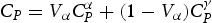
Modelling of recalescence effect on austenite decomposition

Abstract

A model for recalescence has been established by integrating a model for the decomposition of austenite and one dealing with heat transfer with latent heat release taken into account. The effects of recalescence on each individual austenite transformation product have been studied. It was found that Widmanstätten ferrite and pearlite reactions are most affected. The calculated cooling curve, as affected by the recalescence, has also been verified with a commercial steel subjected to two different environment conditions.

Keywords

Recalescence austenite decomposition cooling curve

Introduction

The arrest in the cooling curve of iron has been known in the industry for a very long time, attributed to heat conduction from inside of the object. From 1873 to 1910, Barrett conducted a systematic investigation [1 –3], and proved that it was actually due to the heat release from transformation. He named this phenomenon as ‘recalescence’. The decomposition of austenite to ferrite is accompanied by the release of latent heat, which may cause a temporary rise of temperature when the rate of heat liberation during transformation exceeds that of heat dissipation while cooling the metal through a transformation temperature range.

The phenomenon manifests in the temperature profile which deviates from its original trend when transformation happens, but the most pronounced effects are observed for processes which are unable to increase heat extraction rates when transformations happen, such as natural cooling, or when the section of the object is large, so the heat generated by transformation cannot be removed rapidly.

The latent heat generated by transformation sometimes limits the achievable undercooling which is critical with fine microstructure. Recalescence, thus, limits the minimum grain size achievable by thermomechanical processing to about m [4,5].

The phenomenon is, therefore, significant and the purpose of the present work was to incorporate it into a phase transformation model developed for Si-containing bainitic steels to predict the transformation characteristics of such alloys [6 –12].

Experimental procedure

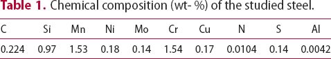
A commercial free-machining steel in the hot-rolled condition was supplied by Swiss Steel AG in the form of rods of 32 mm in diameter, with the chemical composition as listed in Table 1. This alloy is chosen because it is naturally cooled and recalescence has, therefore, been observed routinely in industrial practice.

Table 1

Chemical composition (wt- %) of the studied steel.

C	Si	Mn	Ni	Mo	Cr	Cu	N	S	Al
0.224	0.97	1.53	0.18	0.14	1.54	0.17	0.0104	0.14	0.0042

Test samples of 8 mm in diameter and 10 mm in length were prepared from the hot-rolled bar. All subsequent heat treatments were carried out in a THERMECMASTOR-Z thermomechanical simulator with a vacuum of around 10⁻³ Pa. To investigate recalescence, the sample was heated to 950C, held for 5 min, then followed by natural cooling inside the vacuum chamber; the cooling was achieved by switching off the power and cooling medium supply, so no extra heat input or extraction could be there to affect the heat dissipation process. The temperature of the sample was monitored by a S-type thermocouple spot welded on the middle of the sample during the whole process.

The temperature evolution of mm steel bars cooled naturally in air was measured by Swiss Steel AG. Type K thermocouple was put in a hole drilled in the centre of the bar, and good contact with the bar was maintained by forcing it against the bottom of the hole.

Kinetic model of austenite decomposition

Kinetic model of austenite decomposition is needed to calculate the latent heat released by transformation. A simultaneous phase transformation model, including allotriomorphic ferrite, Widmanstätten ferrite, pearlite and bainite, developed by Jones and Bhadeshia [10,12] and Chen and Bhadeshia, was employed [6,7].

All phases are assumed to nucleate at the prior austenite grain boundaries, and paraequilibrium is assumed, so that only carbon diffusion is considered. The calculation starts with an input of chemical composition, the austenite grain size and the heat treatment scheme. The chemical composition is used to evaluate the driving force for each individual phase transformation using MUCG, a thermodynamic calculation program developed by Bhadeshia [13,14]. The nucleation and growth rates are then calculated separately for each phase. The concentration-dependent carbon diffusivity is calculated as in Bhadeshia [15], Siller and McLellan [16], and Babu and Bhadeshia [17]. The overall transformation kinetics is modelled using the Avrami theory modified for multiple reactions [18 –23].

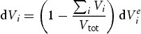
The details are presented elsewhere, and the essential modification to Avrami model is in the conversion between the extend and real space as follows [11,12,24 –26] (1) where is the volume fraction of phase i, is the extended volume fraction of phase i and is the total volume. 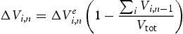These coupled equations are usually too complicated to solve analytically, hence numerical solution is adopted, the volume fraction change of product phase i in the time step is given by (2) where and are the volume fraction changes of phase i at time step n in real and extended space, respectively, is the volume fraction of phase i at step n−1.

The bainite transformation is complicated because it is a displacive transformation with the partitioning of carbon occurring subsequent to the growth event. A simplified model was adopted in this work. The time-temperature-transformation (TTT) diagram for the initiation of reaction is calculated using the method described in Bhadeshia [13,14], then the bainite volume fraction is read from the TTT diagram by a program written for the work. It was also assumed that when bainite starts to form, all reconstructive transformations are stopped, so when transformation temperature is between and temperature, which is also predicted by MUCG [13,14], only bainite transformation is considered.

For carbide-free bainite, which is the focus of this work, excess carbon in the supersaturated bainitic ferrite platelet is partitioned into its surrounding untransformed austenite. is the fraction of untransformed austenite containing of carbon prior to the onset of bainite. where , and are the volume fraction of allotriomorphic ferrite, Widmanstätten ferrite and pearlite, respectively.

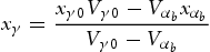
It follows that when bainite forms, the carbon content of austenite is (3) where is the carbon concentration of the untransformed austenite in mole fraction, is that just before bainite transformation starts, is the volume fraction of bainite and is the carbon concentration of bainitic ferrite, which is assumed to be zero.

Assuming paraequilibrium [27], can be used to recalculate the transformation-start time for the untransformed austenite. The calculation is repeated for different bainite volume fractions, this way the whole TTT diagram for bainite can be calculated.

For continuous cooling, the TTT curve is modified using the Scheil's additivity rule [28]. For an apparent bainite volume fraction , for example , of transformation is achieved during continuous cooling when where and are the time spent at the i^th temperature step and the incubation time at the temperature step, respectively.

The temperature range was chosen to be to , or in case of very low temperature, 150C was used as the lower limit, because the transformation time increases dramatically as the temperature is reduced. The actual volume fraction of bainite formed in each step is where is the apparent volume fraction corresponding to the TTT curve under calculation.

Koistinen–Marburger equation [29] is used for martensite transformation. (4) where is the volume fraction of martensite, is the martensite start temperature and is the quenching temperature. The volume fraction of martensite is estimated at different quenching temperatures below , but is scaled by the amount of austenite left untransformed prior to martensite transformation.

Heat transfer model

The product relevant to the present work was produced in a bar form. It was hot-rolled at 1200C followed by natural cooling, with recalescence readily observed. As the kinetic model of austenite decomposition reaction is solved numerically, the step-wise manner of calculation allows the boundary conditions to be updated at every step. By choosing a sufficiently small time step, the heat transfer process can be simplified to a steady state, because the temperature change of the object in a small time interval is also small.

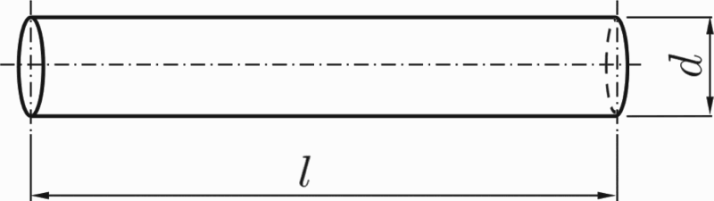
The Biot number (Bi) is used to determine whether or not the temperature varies significantly within the body [30]. (5) where h (W m⁻² K⁻¹) is the heat transfer coefficient, (m) is the characteristic length, (W m⁻² K⁻¹) is the thermal conductivity of the body. The characteristic length is defined as where (m³) is the volume of the body and A (m²) is its surface area. For a long cylinder , where d (m) is the diameter.

indicates that the temperature field can be treated as uniform inside the body [30]. For cooling of the 32 mm diameter steel rod, the measured heat transfer coefficient of air is between 10 and 100 W m⁻² K⁻¹ in the temperature range of 10 to 1000C (Figure 12), take h=100 W m⁻² K⁻¹, m, W m⁻² K⁻¹, so the Bi=0.027<0.1, making it reasonable to neglect the temperature gradient inside the steel bar, in other words, heat transfer into the environment is not controlled by conduction within the bar. By setting Bi=0.1, steel bar of diameter 120 mm can be assumed to have a uniform temperature field.

For steady-state condition, the heat flux q (W m⁻²) is given by Lienhard and Lienhard [30] (6) where (K) is the temperature of the object, (K) is that of the environment.

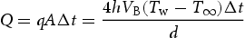
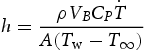
The energy dissipated Q from an object with a surface area of A (m²) in a time interval (s) is

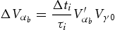
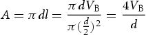
To calculate the heat transfer, the object was chosen to be a steel bar with a diameter d (m), length l (m) and volume (m³) and therefore area 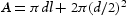(Figure 1).

Figure 1

Geometry of heat transfer model.

Steel bars are usually small in diameter and very long, so the ends can be neglected. The surface area not including the ends is

So the total energy transferred in a time interval is (7)

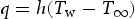
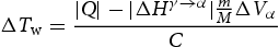
While energy dissipation cools the steel bar, the release of latent heat of transformation heats it up. The temperature change due to the combined effect of heat transfer and latent heat release in the time step is (8) where (J mol is the molar enthalpy change of transformation from austenite to ferrite, is the volume fraction change of ferrite in the time step, m (kg) is the mass of the steel bar, M (kg mol⁻¹) is the molar mass of the alloy, C (J K⁻¹) is the heat capacity of the whole steel bar given by where (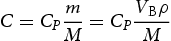J mol⁻¹ K⁻¹) is the molar specific heat capacity of the steel and ρ (kg m⁻³) is the density of the steel.

When transformation happens, the latent heat generated is proportional to the amount of ferrite formed in the very step, the molar specific heat capacity of the mixture of ferrite and austenite is taken to be the weighted average of that of ferrite and austenite: where and are the molar-specific heat capacities of ferrite and austenite, respectively [31,32], and the molar enthalpy change from austenite to ferrite is calculated by the method described below.

Enthalpy calculation

Latent heat is the enthalpy change at the transformation temperature which is a function of temperature and alloy composition. MUCG [13,14] already has the free energy change () as its output. (9) where (J mol⁻¹) is the free energy change, (J mol⁻¹) is the enthalpy change and (J mol⁻¹ K⁻¹) is the entropy change. The latter can be calculated by differentiating with respect to T. Since differentiation is carried out over a small temperature range, the temperature dependence of enthalpy change can be neglected. Then entropy change can be calculated as (10) With and calculated, combine Equations 9 and 10, the enthalpy change can be obtained as (11)

For displacive transformation, must be reduced by the stored energy associated with the transformation strain, 50 J mol⁻¹ for Widmanstätten ferrite, 400 J mol⁻¹ for bainite and 700 J mol⁻¹ for martensite [33].

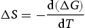
Figure 2(a) shows the enthalpy change for diffusional transformation from austenite to ferrite as a function of temperature for different carbon concentrations. It can be seen that the absolute value of enthalpy change increases with decreasing temperature, but decreases as the carbon content increases, which means that heat released during transformation will be less at high carbon contents and high temperatures. For displacive transformation, the trend is the same, Figure 2(b), but the difference in absolute enthalpy change for the same amount of carbon variation is larger. The enthalpy change of diffusionless transformation is smaller than that of diffusional transformation for the same carbon content at the same temperature, due to the extra carbon trapped in the product phase. The calculated enthalpy change is close to the latent heat of martensite transformation in a medium carbon steel measured by Lee and Lee [34], using an inverse method.

Figure 2

Calculated enthalpy change for austenite to ferrite transformation as a function of temperature (K) and carbon content. (a) Diffusional transformation. (b) Diffusionless transformation. The numbers close to the curves are carbon content in wt- %.

Model Validation

Effect of heat transfer coefficient

The heat transfer coefficient, of course, should have a large effect on recalescence. Calculations using the composition in Table 1 were carried out. Figure 3 shows the calculated cooling curves for different heat transfer coefficient for a variety of time scales. Figure 3(a) shows the calculated cooling curve and volume fraction of allotriomorphic ferrite as a function of time for h=10 W m⁻² K⁻¹. Recalescence is clearly shown, a temperature rise of 10C is predicted at the early stage of transformation where the transformation rate is fast, hence fast heat release rate giving this temperature rise. As the heat transfer coefficient is increased to 100 W m⁻² K⁻¹, the temperature rise is reduced to 5C, shown in Figure 3(b). An increase of h to 500 W m⁻² K⁻¹ leads to a recalescence of just 2C, Figure 3(c). The cooling curves for different heat transfer coefficients are compared in Figure 3(d).

Figure 3

Calculated cooling curve and volume fraction of allotriomorphic ferrite as a function of time. (a) W m⁻² K⁻¹. (b) h= 100 W m⁻² K⁻¹. (c) h=500 W m⁻² K⁻¹. (d) Comparison of cooling curves for different heat transfer coefficients, units of h in the graphs are W m⁻² K⁻¹.

Recalescence effect on the microstructure

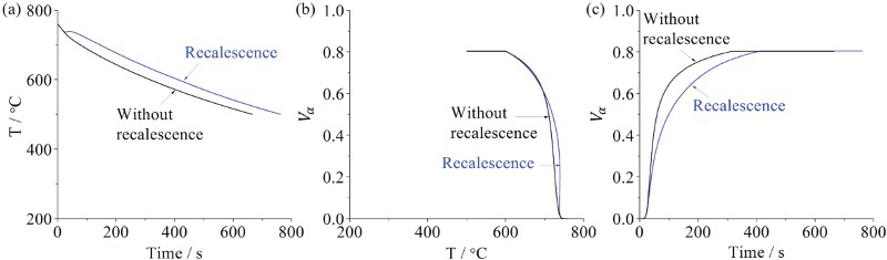
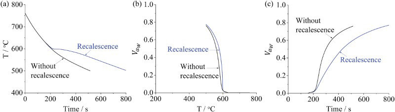
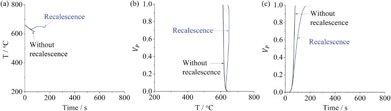
As the cooling curve is affected by the release of latent heat, so should the resulting microstructure. The effects of recalescence on each of the major phase transformations are examined individually in Figures 4–8. For allotriomorphic ferrite, when recalescence of about 2C is considered, the cooling curve is always higher than the one without considering recalescence after the initiation of transformation. Figure 4(a–c) shows that recalescence retards the transformation. Compared with allotriomorphic ferrite, Widmanstätten ferrite has a much greater change in cooling curve due to recalescence, because it forms at a lower temperature where the enthalpy change is greater, in addition, the heat transfer coefficient is smaller at low temperatures. But there is no temperature rise due to the small growth rate compared to that of allotriomorphic ferrite. To investigate pearlite, the carbon content was changed to the eutectoid content of 0.8 wt- %, the resulting cooling curve of pearlite with recalescence has a temperature rise of 20C, which is much larger than that of allotriomorphic ferrite. 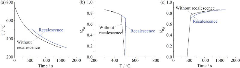Even though higher carbon content should give smaller molar enthalpy change, but transformation happened at lower temperature, at about 620C compared to 740C for allotriomorphic ferrite, which generates larger latent heat. Most importantly, the growth rate is very large, which can be tens of microns per second and the transformation happens in a narrow temperature range, Figure 6, consistent with reports from the literature [35 –42]. Bainite follows the same trend, and the rise in temperature is about 7C. The exception is martensite, which was assumed to be athermal, therefore, the volume fraction depends only on temperature, and the release of latent heat reduces only the cooling rate, making the time to reach the same temperature longer. If the latent heat release rate is larger than the heat dissipation rate, martensite transformation will be stopped by the temperature increase, until temperature cools below the instantaneous temperature, where the transformation can be resumed.

Figure 4

Effect of recalescence on allotriomorphic ferrite transformation.

Figure 5

Effect of recalescence on Widmanstätten ferrite transformation.

Figure 6

Effect of recalescence on pearlite transformation.

Figure 7

Effect of recalescence on bainite transformation.

Figure 8

Effect of recalescence on martensite transformation.

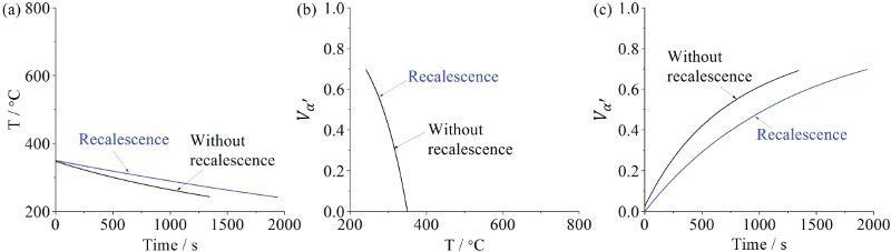
We now consider phase transformations that can happen simultaneously. Table 2 shows the calculated microstructures for different austenite grain sizes with and without recalescence. The composition used in the calculation is 0.18C-0.18Si-1.15Mn wt- % from Jones (1996) [10], and the heat transfer coefficient is shown in Equation (13). For austenite grain sizes of 10 µm and 30 µm, the difference due to recalescence is small, Figure 9. For larger austenite grain sizes where the reaction rates are relatively slow, considerable differences in microstructure were found, Figure 10. It is well known that the portion of Widmanstätten ferrite increases with the prior austenite grain size [43,44] and recalescence exaggerates this because the cooling rate is considerably reduced. This also affects the remaining austenite which eventually transforms into pearlite. It could also be possible for other alloys or cooling conditions where high temperature products will not transform all the austenite, so bainite and martensite should form as well, and the resulting microstructure could be remarkably different. These calculations show that it is important to consider recalescence for modelling of microstructure development.

Figure 9

Effect of recalescence on simultaneous transformation with m. (a) Comparison of cooling curves with and without recalescence taken into account. (b) and (c) Microstructure evolutions for the cases of without and with recalescence considered, respectively.

Figure 10

Table 2

Comparison of calculated phase fractions, with and without recalescence taken into account.

	Allotriomophic ferrite		Widmanstatten ferrite		Pearlite
Grain size/µm	With	Without	With	Without	With	Without
10	0.75	0.74	0	0	0.25	0.26
30	0.60	0.58	0.01	0.03	0.39	0.39
50	0.45	0.40	0.41	0.24	0.14	0.36
100	0.25	0.24	0.49	0.39	0.26	0.37

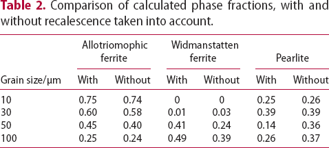
Experimental validation of cooling curve prediction

The bainite start temperature of the steel was measured to be C, Figure 11, using the offset method [45]. Recalescence was observed clearly in the measured cooling curve, shown in Figure 13. At around 450C, the cooling curve starts to deviate from its original trend, which is caused by bainite formation, verified by metallographic examination.

Figure 11

Strain versus temperature curve for mm cylindrical sample freely cooled from 950C in the THERMECMASTOR-Z simulator under vacuum.

Figure 12

Comparison of heat transfer coefficients for the two different conditions, black line for mm bar cooled naturally in air, blue line for mm sample cooled freely inside the simulator under vacuum.

Figure 13

Comparison of calculated and measured cooling curves for mm sample cooled freely from 950C in THERMECMASTOR-Z under vacuum.

The temperature-dependent heat-transfer coefficient can be obtained by Holman [46] and Kreith [47] (12) where is the instantaneous cooling rate.

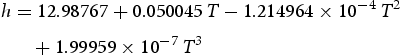
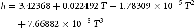
The measured heat transfer coefficient as a function of temperature is shown in Figure 12, the fitted equation for mm cylindrical sample in THERMECMASTOR-Z under vacuum is (13) where h is in W m⁻² K⁻¹, T is in C.

For the mm steel bar cooled in air, the heat transfer coefficient is (14)

Predictions were made using these heat transfer coefficients. Figure 13 shows the calculated cooling curve with and without transformation latent heat included for the mm sample transformed in THERMECMASTOR-Z under vacuum, the transformation start temperature used was the experimentally measured C. The comparison with the measured cooling curve is also shown in Figure 13; the calculated curve did not follow the measured curve at the transformation start point, where the measured curve deviated much more than the calculated, but after some time, the calculated curve converged with the measured one, where the calculated transformation finishes. The discrepancy occurs because the calculated rate of bainite formation is slower than experimental value; as shown in Figure 11, the bainite actually formed in a very narrow temperature range, mostly between 440C and 390C, and the rate of transformation in that range is larger than the calculated. Figure 14 shows the calculated and measured cooling curve for the mm bar cooled in air. Fairly good closure between calculation and experimental measurement is obtained.

Figure 14

Comparison of the calculated and measured cooling curves for mm rod cooled naturally in air.

Conclusions

A recalescence model has been developed by integrating a heat transfer model into the simultaneous phase transformation model. The effect of latent heat release on each individual phase transformation and multiple transformations happening simultaneously has been studied.

The model has successfully estimated the recalescence phenomenon, and the trend for increasing heat transfer coefficient was demonstrated.

Microstructure is affected by recalescence, and the extent depends on the actual condition. Recalescence retards transformation by reducing the cooling rate, but the transformation finishes at higher temperature. For simultaneous transformations, if Widmanstätten ferrite and pearlite present the microstructure can be influenced significantly.

The pearlite transformation starts at relatively lower temperatures compared to that of allotriomorphic ferrite, where the latent heat evolved is larger and the heat transfer coefficient is smaller. These factors combined with its large growth rate result in the pearlite transformation giving the largest temperature rise among all transformations.

For the cooling curve estimation, reasonable agreement between prediction and experiment has been achieved using the measured transformation start temperature. Therefore, it is necessary to utilise recalescence to give a more accurate representation of the temperature evolution during the course of transformation, hence a better prediction of microstructure could be achieved. However, it is emphasised that while the treatment of recalescence is generic, the heat transfer coefficients have to be measured for particular processing conditions.

Footnotes

Disclosure statement

No potential conflict of interest was reported by the authors.

ORCID

L. Guo

M. Lembke

References

Barrett

. Historical note on recalescence. Nature. 1910;85:235–236. doi: 10.1038/085235e0

Barrett

. Historical note on recalescence. Nature. 1899;60:173. doi: 10.1038/060173b0

Barrett

. LXII. On certain remarkable molecular changes occurring in iron wire at a low red heat. Philos Mag Ser 4. 1873;46:472–478.

Yokota

, Mateo

, Bhadeshia

HKDH

. Formation of nanostructured steels by phase transformation. Scr Mater. 2004;51:767–770. doi: 10.1016/j.scriptamat.2004.06.006

Bhadeshia

HKDH

. 52nd hatfield memorial lecture large chunks of very strong steel. Mater Sci Technol. 2005;21:1293–1302. doi: 10.1179/174328405X63999

Chen

, Bhadeshia

, Hasler

, et al. Complete calculation of steel microstructure for strong alloys. Proc New Dev Metall Appl High Strength Steels, Buenos Aires. 2008;2:749–759.

Chen

. Modelling of simultaneous transformations in steels [Ph.D. thesis]. University of Cambridge; 2009.

Guo

, Roelofs

, Lembke

, et al. Modelling of transition from upper to lower bainite in multi-component system. Mater Sci Technol. 2016. DOI:10.1080/02670836.2016.1221495.

Guo

, Roelofs

, Lembke

, et al. Effect of manganese sulphide particle shape on the pinning of grain boundary. Mater Sci Technol. 2016. DOI:10.1080/02670836.2016.1258157.

10.

Jones

. Modelling inclusion potency and simultaneous transformation kinetics in steels [Ph.D. thesis]. University of Cambridge; 1996.

11.

Jones

, Bhadeshia

HKDH

. Competitive formation of inter-and intragranularly nucleated ferrite. Metall Mater Trans A. 1997;28:2005–2013. doi: 10.1007/s11661-997-0157-8

12.

Jones

, Bhadeshia

HKDH

. Kinetics of the simultaneous decomposition of austenite into several transformation products. Acta Mater. 1997;45:2911–2920. doi: 10.1016/S1359-6454(96)00392-8

13.

Bhadeshia

HKDH

. MAP_STEEL_MUCG46. 1982. Available from: http://www.msm.cam.ac.uk/map/steel/programs/mucg46-b.html.

14.

Bhadeshia

HKDH

. Thermodynamic analysis of isothermal transformation diagrams. Metal Sci. 1982;16:159–166. doi: 10.1179/030634582790427217

15.

Bhadeshia

HKDH

. Diffusion of carbon in austenite. Metal Sci. 1981;15:477–480. doi: 10.1179/030634581790426525

16.

Siller

, McLellan

. The variation with composition of the diffusivity of carbon in austenite. Trans Met Soc AIME. 1969;245:697–700.

17.

Babu

, Bhadeshia

HKDH

. Diffusion of carbon in substitutionally alloyed austenite. J Mater Sci Lett. 1995;14:314–316. doi: 10.1007/BF00592135

18.

Kolmogorov

. On statistical theory of metal crystallisation (Izvestiya Akad Nauk SSSR (Izvestia Academy of Science, USSR). Ser. Math. 1937;3:335–360.

19.

Johnson

, Mehl

. Reaction kinetics in processes of nucleation and growth. Trans AIME. 1939;135:396–415.

20.

Avrami

. Kinetics of phase change. I. General theory. J Chem Phys. 1939;7:1103–1112. doi: 10.1063/1.1750380

21.

Avrami

. Kinetics of phase change. II. Transformation-time relations for random distribution of nuclei. J Chem Phys. 1940;8:212–224. doi: 10.1063/1.1750631

22.

Avrami

. Granulation, phase change, and microstructure kinetics of phase change. III. J Chem Phys. 1941;9:177–184. doi: 10.1063/1.1750872

23.

Christian

. Theory of transformations in metals and alloys, Part I. 3 ed. Oxford: Pergamon Press; 2003.

24.

Robson

, Bhadeshia

HKDH

. Modelling precipitation sequences in power plant steels: part I, kinetic theory. Mater Sci Technol. 1997;13:631–639. doi: 10.1179/mst.1997.13.8.631

25.

Robson

, Bhadeshia

HKDH

. Modelling precipitation sequences in power plant steels, Part 2: application of kinetic theory. Mater Sci Technol. 1997;28A:640–644. doi: 10.1179/mst.1997.13.8.640

26.

Robson

, Bhadeshia

HKDH

. Kinetics of precipitation in power plant steels. CALPHAD. 1996;20:447–460. doi: 10.1016/S0364-5916(97)00007-2

27.

Bhadeshia

HKDH

. Bainite in steels: theory and practice. 3rd ed. Leeds: Maney Publishing; 2015.

28.

Scheilk

. Anlaufzeit der austenitumwandlung. Archiv für das Eisenhüttenwesen. 1935;8:565–567. doi: 10.1002/srin.193500186

29.

Koistinen

, Marburger

. A general equation prescribing the extent of the austenite-martensite transformation in pure iron–carbon alloys and plain carbon steels. Acta Metallurgica. 1959;7:59–60. doi: 10.1016/0001-6160(59)90170-1

30.

Lienhard

, Lienhard

. A heat transfer textbook. Cambridge (MA): Phlogiston Press; 2000.

31.

Kaufman

, Clougherty

, Weiss

. The lattice stability of metals – III. Iron. Acta Metall. 1963;11:323–335. doi: 10.1016/0001-6160(63)90157-3

32.

Kaufman

. Condensed state reactions at high pressures. In: Mueller WM, editor. Energetics in metallurgical phenomena, vol. III. New York: Gordon and Breach; 1967. p. 53.

33.

Bhadeshia

HKDH

. Bainite in steels. 2nd ed. London: Institute of Materials; 2001.

34.

Lee

S-J

, Lee

Y-K

. Latent heat of martensitic transformation in a medium-carbon low-alloy steel. Scr Mater. 2009;60:1016–1019. doi: 10.1016/j.scriptamat.2009.02.042

35.

Brown

, Ridley

. Rates of nucleation and growth and interlamellar spacings of pearlite in a low-alloy eutectoid steel. J Iron Steel Inst. 1966;204:811–816.

36.

Brown

, Ridley

. Kinetics of the pearlite reaction in high-purity nickel eutectoid steels. J Iron Steel Inst. 1969;207:1232–1240.

37.

Pandit

, Bhadeshia

HKDH

. Mixed diffusion-controlled growth of pearlite in binary steel. Proc Roy Soc A. 2011;467:508–521. doi: 10.1098/rspa.2010.0210

38.

Pandit

, Bhadeshia

HKDH

. The growth of pearlite in ternary steels. Proc Roy Soc A. 2011;467:2948–2961. doi: 10.1098/rspa.2011.0165

39.

Pandit

, Bhadeshia

HKDH

. Divorced pearlite in steels. Proc Roy Soc A. 2012;468:2767–2778. doi: 10.1098/rspa.2012.0115

40.

Pandit

. Theory of the pearlite transformation in steels [Ph.D. thesis]. Pembroke Street, Cambridge CB2 3QZ: University of Cambridge, Department of Materials Science and metallurgy; 2011.

41.

Seo

S-W

. Pearlite growth rate in Fe-C binary and Fe-C-X ternary steels [Ph.D. thesis]. Pohang University of Science and Technology, Graduate Institute of Ferrous Technology; 2015.

42.

Seo

S-W

, Bhadeshia

HKDH

, Suh

D-W

. Pearlite growth rate in Fe-C and Fe-Mn-C steels. Mater Sci Technol. 2015;31:487–493. doi: 10.1179/1743284714Y.0000000641

43.

Bodnar

, Hansen

. Effects of Widmanstätten ferrite on the mechanical properties of a 0.2 pct C-0.7 pct Mn steel. Metall Mater Trans A. 1994;25:763–773. doi: 10.1007/BF02665453

44.

Bodnar

, Hansen

. Effects of austenite grain size and cooling rate on Widmanstätten ferrite formation in low-alloy steels. Metall Mater Trans A. 1994;25:665–675. doi: 10.1007/BF02665443

45.

Yang

H-S

, Bhadeshia

HKDH

. Uncertainties in dilatometric determination of martensite start temperature. Mater Sci Technol. 2007;23:556–560. doi: 10.1179/174328407X176857

46.

Holman

. Heat transfer. New York: McGraw Hill; 2004.

47.

Kreith

, editor. Mechanical engineering handbook. Florida: CRC Press LLC; 1999.