Comparison of baseline method and DSC measurement for determining phase fractions

Abstract

By comparing phase fractions upon solidification of Ni–3·3 wt-B alloy obtained by differential scanning calorimetry (DSC) measurement, microstructure observation and the baseline method, the results show that although as an approximate approach, the baseline method can be used to predict the phase fractions from the cooling curve, and it can reflect the relationship between the transformed fraction, time and temperature simultaneously during solidification, which cannot be obtained from DSC measurement. In addition, the effects of non-constant specific heat and latent heat of phases on the baseline method are discussed and the calibration relationships are deduced.

Keywords

Baseline Transformed fraction Solidification Cooling curve

Introduction

Upon solidification with negligible undercooling, the transformed fraction can be directly measured using differential thermal analysis (DTA), differential scanning calorimetry (DSC), synchrotron diffraction or dilatometry experiments,1,2 whereas for rapid solidification, delicately and repeatedly treating the sample is essential for achieving a high undercooling; in this case, most of the above techniques are limited due to the expensive facilities.3^–5 Furthermore, the temperature changes rapidly during the recalescence process for undercooled solidification, and the actual thermal history of the sample is not shown in the DTA or DSC curve. Therefore, the actual cooling curves with transformed fraction cannot be obtained from thermal analysis technologies.

As an inexpensive approach, the cooling curve method provides consistent results reflecting the solidification process.3^–12 Computer aided cooling curve thermal analysis (CA-CCA) is a common method to evaluate the solidification from thermal history. Stefanescu et al. used CA-CCA method by coupling the macroscopic heat transfer and microscopic kinetics to calculate the solid fraction during solidification.6 Emadi et al. analysed the cooling curve of Al–Si alloy using the CA-CCA method.7 Recently, applying first principles analysis of thermodynamics and heat flow, Gibbs et al. developed a method to study the cooling curves of Al–Si and Al–Ag alloys.1 However, all of these methods need the derivative of the cooling curves.1,6,7 In this case, accuracy of the results is often impaired by the large noise of the derivative curve. Accordingly, with the assumption of constant specific heat and latent heat of phases, a baseline method to determine directly the transformed fraction using the cooling curve has been proposed for solidification of undercooled melts.5

In the present study, we will compare the transformed fraction obtained from the baseline method with that from the DSC measurement (and the microstructure observation) for Ni–3·3 wt-B alloy. Effects due to change of specific heat and latent heat of phases on the baseline method will be discussed.

Experimental

To investigate the undercooled solidification of Ni–3·3 wt-B alloy, the sample, weighing ∼4 g, together with some pieces of B₂O₃ glass, was placed into a quartz glass crucible, which was placed in the middle position of the high frequency induction coil located in a vacuum chamber. After the vacuum chamber was evacuated to 1×10⁻⁶ mbar and backfilled to 600 mbar with high purity Ar gas, the sample was cyclically superheated with a superheating 100–200 K until a desired undercooling was achieved. Thermal history of samples was monitored by a one-colour pyrometer. For morphology observation, a solution consisting of 5 g FeCl₃, 10 mL HCl and 50 mL H₂O was used to etch the as solidified specimens. For DSC experiment, a sample weighing ∼8 mg was put in the alumina crucible, and it is heated with 10 K min⁻¹ from 1173 to 1573 K to measure the melting point. Then, the sample is cooled with the rate of 40 K min⁻¹ from 1573 to 600 K to measure the characteristic temperatures.

Theoretical description

Transformed fraction

To analyse the thermal history for solidification of an alloy, the following assumptions are made:

the specimen undergoing solidification is spherical

both values of the specific heat before and after the solidification hold constant

iii

solidification in the present study is assumed to be completed within short freezing range, where the rate of heat extraction can be considered as constant

the contribution from radiation is neglected

the temperature gradient inside the particle is negligible during cooling.

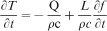
Regarding the above assumptions, a combination of the heat capacity, the released latent heat and the heat transfer to environment leads to an equation of heat balance3,4 (1) where f is the solid fraction, T is the melt temperature, L is the latent heat of solidification, Q is the heat extraction rate due to radiation and convection and ρc is the volume heat capacity.

Accordingly, an analytical solution of equation (1) can be assumed as (2) with

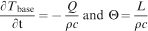
At the right hand side of equation (2), the first term stands for the liquid/solid cooling process without latent heat release (analogous to the process of glass formation), i.e. the baseline, and the second term stands for the latent heat releasing process without cooling (analogous to an adiabatic process). Thus, the solidification can be considered as an addition of the two extreme processes.

Baseline equation

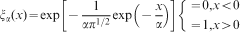
To describe the baseline, a sudden function ξ_α(x) is introduced as5 (3a) where α is constant. For sufficiently small α (α = 0·1 is assumed here), ξ_α(x) is nearly straight from zero to one at x = 0. From equation (3a), it can be deduced as (3b) Both equations (3a) and (3b) are generally used to describe the event such as the baseline for cooling curve upon solidification.

To illustrate the baseline equation, Fig. 1 shows the schematic thermal history of solidification, where the solidification is initiated at point A (liquid state in OA stage) and completed at point C (solid state in CD stage). Without releasing latent heat upon solidification, the sample should transform directly from liquid to solid, i.e. the temperature varies along the baseline OAF (where AF is parallel to CD), the baseline OAEG (where AE is the extension of OA, EG parallel to CD) or the baseline T_base(t) between OAF and OAEG, to the room temperature. Actually, the latent heat release must be considered, and accordingly, the solid cooling curve CD delays duration of time Δt and goes down to room temperature (Fig. 1). Since Δt is related to the latent heat release, the temperatures rising ΔT can be regarded as the distance between a point at the cooling curve OABCD and the corresponding point at the baseline OAF, OAEG or T_base(t), and stands for the degree of latent heat released. As the baseline T_base(t) is difficult to determine, the two extreme baselines (OAF and OAEG) are dealt with first:

Figure 1

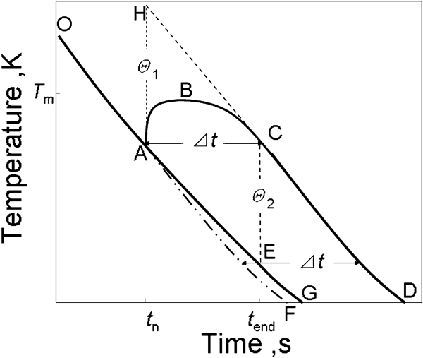
Schematic thermal history of solidification

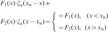
elongate DC to H (corresponding to the initial nucleation time t_n); move DCH down Θ₁ to A (Fig. 1), and the baseline OAF is obtained. From equation (3b), the baseline OAF can be expressed as (4a)

elongate OA to E (corresponding to the solidification ending time t_end); move CD down Θ₂ to E (Fig. 1), and the baseline OAEG is obtained. From equation (3b), the baseline OAEG can be expressed as (4b) For an ideal case where the cooling rates of liquid and solid are equivalent and constant, the two baselines are completely overlapped.

From Refs. 3, 4, and 12, pure liquid part, OA(t), or pure solid part, CD(t), of cooling curve can be expressed as (T₀−T_G)exp [−h(C_pR/3)⁻¹(t−t₀)]+T_G = Aexp (−Bt)+T_G, where T₀ is the initial temperature at the beginning of time interval t₀. T_G is the environment temperature; h is the heat transfer coefficient at the specimen/environment interface; R is the specimen radius; and A and B are constants. Thus (5a) (5b) where A_l,B_l and A_s,B_s are constants for pure liquid and pure solid respectively.

Whole expression for baseline method

From the descriptions above, several kinds of baseline methods can be given.

First, assume the baseline is T_base1, according to equations (2), (4a), (5a) and (5b) (6a) (6b) (6c) where T is the temperature of cooling curve, t is time, t_n is the initial solidification time and T(t_n) is the initial solidification temperature.

Assume the baseline is T_base2, according to equations (2), (4b), (5a) and (5b) (7a) (7b) (7c) where t_end is the finish solidification time and T(t_end) is the finish solidification temperature.

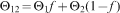
Second, considering the effect of transformed fraction on the baseline, a synthetic method results as (8a) (8b) (8c) Third, if Θ₁ equals to Θ₂, the three baselines will be totally the same, i.e. T_base1 = T_base2 = T_base = Φ _l. Then, equations (6a), (7a) and (8a) will return to the same expression (9) Therefore, by equations (5)–(9), the transformed fraction can be predicted directly from the cooling curve, where the fitting parameters are A_l,B_l, A_s and B_s. Then, with the values of B_l or B_s, and the specimen radius R, the average heat transfer coefficient at the specimen/environment interface, h can be determined. With the start and the end points (obtained from cooling curves) of the phase transformations, the fractions of different phases can be estimated.

Calibration of phase fraction

For baseline method, arbitrary assumption of constant specific heat and latent heat for different phases (the average values are used) may lead to deviation from the experimental results. In fact, both of them are not constant during the solidification process. Considering the change of specific heat and the latent heat, a calibration of the calculated results from baseline method will be deduced.

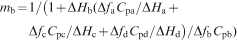
Taking solidification including two transformations as an example, after the first phase formation, the actual fraction and the latent heat of the first phase and the specific heat of the whole alloy are m_a, ΔH_a and C_pa respectively; after the second phase formation, the actual fraction and the latent heat of the second phase and the specific heat of the whole alloy are m_b, ΔH_b and C_pb respectively. Assume the transformation as an adiabatic process, the latent heat releases of the first and the second phases lead to the temperature of the system rise ΔT_a ( = m_aΔH_a/C_pa) and ΔT_b ( = m_bΔH_b/C_pb) respectively. Accordingly, ΔT_a: ΔT_b = m_aΔH_a/C_pa: m_bΔH_b/C_pb.

From the present baseline method, the fractions of the first and the second phases can be determined as Δf_a and Δf_b. Since baseline method is on the basis of the temperature rising (ΔT_a and ΔT_b) due to the latent heat release, it can be deduced Δf_a: Δf_b = ΔT_a: ΔT_b = m_aΔH_a/C_pa: m_bΔH_b/C_pb. For solidification with two transformations, due to Δf_a+Δf_b = 1 and m_a+m_b = 1, the actual fractions m_a and m_b can be determined as (10a) (10b) Thus, if the latent heat and specific heat are known, equation (10) can be used to calibrate the phase fraction from the baseline method (equations (5)–(9)).

For solidification with three or more transformations, considering the change of specific heat and latent heat for different phases, an analogous calibration method is available. For example, for solidification with four transformations, the calibration relationship for the real fraction of every phase can be expressed as (11a) (11b) (11c) (11d) where the subscripts a, b, c and d denote the variables (m, ΔH and Δf) of the first, second, third and fourth phases, and C_pa–C_pd stand for the specific heat of the system when the four phases are formed respectively. From equation (11), it can be seen that if ΔH_a/C_pa = ΔH_b/C_pb = ΔH_c/C_pc = ΔH_d/C_pd, m_a, m_b, m_c and m_d will equal to Δf_a, Δf_b, Δf_c and Δf_d respectively.

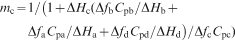
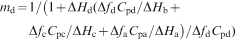
Accordingly, the general calibration relationship for different phases can be written as (12) For the present calibration, the specific heat of the system for different temperature, C_pi, and the latent heats for different phases, ΔH_i, are required parameters. Generally, the differences of the latent heats for different phases in the alloy system are not obvious; the variation of specific heat can be neglected so the transformed fractions from the baseline method without calibration are close to the actual results.

Applications

Cooling curve and microstructure of rapid solidification of Ni–3·3 wt-B alloy

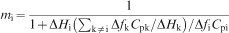
The cooling curve of Ni–3·3 wt-B alloy is shown in Fig. 2a. Since the maximal recalescence temperature for eutectic solidification is ∼1234 K, which is far less than the equilibrium eutectic (Ni–Ni₃B) temperature (1366 K), but near the metastable eutectic (Ni–Ni₂₃B₆) temperature (1261 K), it is solidified according to the non-equilibrium phase diagram.13^–17 The primary solidification occurs at ∼1330 K, where the primary phase is α-Ni according to the non-equilibrium phase diagram. Then, the metastable eutectic reaction occurs at 1234 K and the rod eutectic phase (Ni–Ni₂₃B₆) forms. Generally, Ni₂₃B₆ phase cannot be kept into room temperature13,14 so that a solid state decomposition Ni₂₃B₆→Ni₃B+Ni must occur in subsequence. Meanwhile, the Ni₃B from decomposition will activate the reaction L_r→Ni₃B+Ni (L_r is the residual liquid), so the reactions in the third recalescence of cooling curve initiated at ∼1190 K are Ni₂₃B₆→Ni₃B+Ni and L_r→Ni₃B+Ni (Fig. 2a). As a result, the microstructure of this sample, as shown in Fig. 2b, consists of primary α-Ni, dot phases (rod eutectic+precipitates), matrix (Ni₃B) and network boundary (anomalous eutectic). α-Ni is from the primary solidification L→α-Ni (corresponding to the first recalescence of the cooling curve). One of the dot phases (rod eutectic) with a regular distribution and the larger size comes from the metastable eutectic transformation L→Ni₂₃B₆+Ni (corresponding to the second recalescence of the cooling curve); the other (precipitates) with irregular distribution and nanosize is a product of the decomposition Ni₂₃B₆→Ni₃B+Ni. The network boundary is the product of the transformation of L_r→Ni₃B+Ni (corresponding to the third recalescence of the cooling curve).17

Figure 2

a cooling curve of Ni–3·3 wt-B alloy and b corresponding microstructure

Determination of transformed fraction

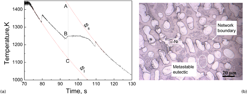
Figure 3 shows the derivative of cooling curves in Fig. 2a, i.e. cooling rate dT/dt versus time t. It can be seen that the noise of the curve is very large. Since the baseline (representing no phase change) of CA-CCA method should be from the derivative of cooling curves,1,2 the error of the calculating result from CA-CCA method will be great.

Figure 3

Derivative curve of cooling curve in Fig. 2a

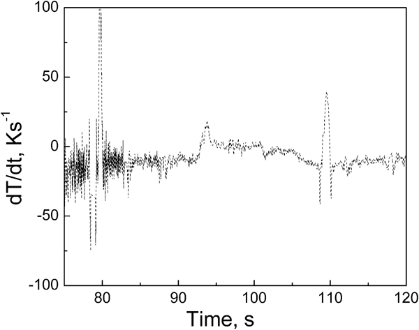
From the present baseline method, given the environment temperature T_G = 350 K, t_n = 79·49 s, t_end = 109·7 s, by fitting with equations (5a) and (5b), the liquid part and the solid part of cooling curves can be expressed as Φ_l = 3434exp (−0·0158t)+350 and Φ_s = 4219exp (−0·0144t)+350. By equations (6) and (7), we can obtain Θ₁ = 360 K and Θ₂ = 258 K, T_base1 = Φ_lξ _α (79·49−t)+(Φ_s−Θ₁)ξ_α(t−79·49)and T_base2 = Φ_lξ _α (109·7−t)+(Φ_s−Θ₂)ξ _α (t−109·7).

As shown in Fig. 4a, the transformed fractions f₁ (corresponding to T_base1), f₂ (corresponding to T_base2) and f₃ can be determined from equations (6a), (7a) and (9) respectively. Figure 4b shows transformed fractions as a function of temperature. The difference between f₁ and f₂ is very small so that it does not need to further calculate f by equation (8a) (since the value of f is always between f₁ and f₂).5 From the curves of f₁, f₂ and f₃, the primary solidification finished at f₁ = 39, f₂ = 36 and f₃ = 32 respectively; the metastable eutectic solidification finished at f₁ = 92, f₂ = 90 and f₃ = 90 respectively. After then, the solid state transformation begins and finished at f₁ = f₂ = f₃ = 1. Assuming the phase fractions are identical to the fractions of heat release due to transformations, the fraction of primary phase is determined to be 32–39 from the baseline method; the fraction of the network boundary is determined to be 8–10. The microstructure in Fig. 2b shows that the fraction of primary phase (α-Ni) is about 30–40; the fraction of network boundary is about 5–10. As a result, the predicted phase fractions from equations (6)–(9) are close to the observation of microstructure. It is worth noting that although equation (9) is a rough method,5 the prediction of primary phase (32) has a slight difference with that from f₁ and f₂ (Fig. 4).

Figure 4

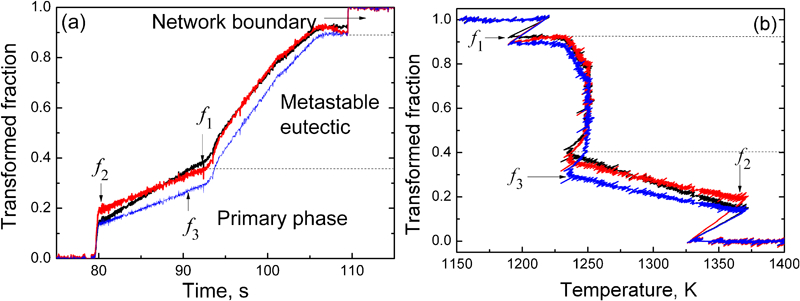
Transformed fractions calculated from equations (6a), (7a) and (9) respectively

DSC study

In order to determine the volume fractions of the respective phases in the microstructure, DSC investigation was utilised. Figure 5 shows the DSC curve of Ni–3·3 wt-B alloy. Upon heating, only one recalescence peak occurs in the DSC curve, where the onset point is observed as ∼1366 K, consistent with the equilibrium eutectic temperature (1366 K) in the Ni–Ni₃B phase diagram. The melting enthalpy is calculated to be ∼128·58 kJ kg⁻¹. Upon cooling, the first, second and third transformations initiate at ∼1420, 1221 and 1110 K, which are close to the first, second and third transformations respectively of the cooling curve in Fig. 2a. It indicates that the solidification of DSC sample is also according to the non-equilibrium phase diagram.13,14 Generally, if the compositions of the samples do not change and the solidification conditions are similar, the phase fractions will also be approximately equal. As a result, in the cooling process of DSC experiment, the first, second and third peaks correspond to the primary solidification (L→α-Ni), metastable eutectic solidification (L→Ni₂₃B₆+Ni) and transformations of Ni₂₃B₆→Ni₃B+Ni and L_r→Ni₃B+Ni respectively. The measured enthalpy of the three peaks are ∼53·3 kJ kg⁻¹, 81·5 kJ kg⁻¹ and 13·1 kJ kg⁻¹ respectively. Here, we also assumed that the phase fractions are identical to the fractions of heat release due to transformations. Accordingly, from DSC measurement, the primary solidification finished at f = 36·04; the metastable eutectic solidification finished at f = 81·14; then, the residual liquid transformation finished at f = 1. Thus, the fractions of α-Ni phase, metastable eutectic phase and the network boundary (from solidification of residual liquid) are determined by the values of enthalpy to be ∼36·04, 55·10 and 8·86 respectively. It is approximately equal to the observation of microstructure in Fig. 2b.

Figure 5

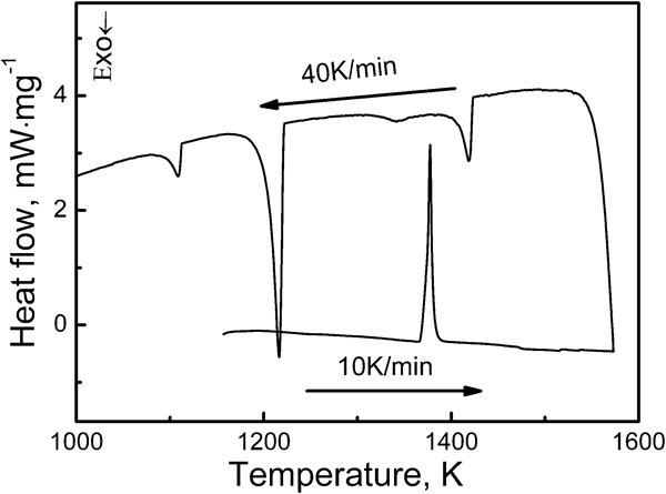
DSC curve of Ni–3·3 wt-B alloy

Comparing the calculations from equations (6)–(9) with the DSC result, it is shown that equations (6)–(8) can acquire more accurate transformed fraction (near the DSC measurement); equation (9) is the simplest one of them, being similar to the level rule, though the error from equation (9) is usually relatively high.5 According to equation (9), as shown in Fig. 2a, the transformed fraction of any point, B, in the cooling curve can be estimated directly by f₃ = BC/AC.

From the calculated results of the present study and that in Ref. 5, the phase fractions from the baseline method without calibration are consistent with the microstructure observation or the calculated results from available methods, which may indicate that variations of the latent heat of different phases and the specific heat of alloys in the present study are not obvious in solidification.

The present model assumes that when a second solid phase begins to form, the first phase remains at its final value. Thus, it is not applicable to the transformation that the first phase does not stop when the second phase begins

Conclusions

The transformed fraction of undercooled solidification Ni–3·3 wt-B alloy estimated by baseline method coincides with that from DSC measurement and observation of the microstructure, which confirms that it is an approximate but convenient method to predict the phase fraction for general undercooled experiment. The present method can give the relationship between the transformed fraction and temperature during solidification, which cannot be obtained from DSC measurement. In addition, the calibration relationships for the variations of specific heat and latent heat are deduced.

Footnotes

Acknowledgements

The authors are grateful for the financial support of the China National Funds for Distinguished Young Scientists (grant no. 51125002), the Natural Science Foundation of China (grant nos. 50901059, 51071127 and 51134011), the National Basic Research Program of China (973 Program) (grant no. 2011CB610403), the Free Research Fund of State Key Laboratory of Solidification Processing (grant nos. 09-QZ-2008 and 24-TZ-2009) and the 111 project (project no. B08040).

References

Gibbs

, Kaufman

, Hackenberg

, Mendez

: Metall. Mater. Trans . A , 2010, 41A, 2216–2223.

Kumar

, Lakshmi

, Dutta

: J. Therm. Sci. Eng. Appl. , 2012, 4, 011006.

Levi

, Mehrabian

: Metall. Trans. B , 1980, 11B, 21–27.

Levi

, Mehrabian

: Metall. Trans. A , 1982, 13A, 221–234.

, Liu

, Xu

, Chen

: Metall. Trans. A , 2012, 43A, 1268–1276.

Stefanescu

, Upadhya

, Bandyopadhyay

: Metall. Trans. A , 1990, 21A, 997–1005.

Emadi

, Whiting

, Djurdjevic

, Kierkus

, Sokolowski

: MJoM , 2004, 10, 91–106.

Barth

, Joo

, Wei

, Herlach

: J. Non-Crys t. Solids , 1993, 156–158, 398–401.

Çetin

, Kalkanli

: Can. Metall. Q. , 2005, 44, 1–6.

10.

Vedovato

, Zambon

, Ramous

: Mater. Sci. Eng. A , 2001, A304–A306, 235–239.

11.

Saleh

, Clemente

: Jpn J. Appl. Phys. , 2004, 43, 3624–3628.

12.

Gandin

Ch.-A

, Mosbah

, Volkmann

, Herlach

: Acta Mater. , 2008, 56, 3023–3035.

13.

Baricco

, Ferrari

, Battezzati

: Mater. Res. Soc. Symp. Proc. , 1996, 398, 81–86.

14.

Battezzati

, Antonione

, Baricco

: J. Alloys Compd , 1997, 247, 164–171.

15.

Ajao

, Hamar-Thibault

, Thibault-Desseaux

: J. Mater. Sci. , 1989, 24, 3647–3659.

16.

Ajao

, Hamar-Thibault

: J. Mater. Sci. , 1988, 23, 1112–1125.

17.

Liu

, Xu

: ‘Undercooled solidification of Ni–3·3wt.B alloy’, Adv. Mater. Res. , 2012, 562–564, 15–18.