Parameters prediction in additively manufactured Al-Cu alloy using back propagation neural network

Abstract

The relationship between tensile strength, wire feeding speed and travel speed is built based on Back Propagation (BP) neural network during the wire arc additive manufacturing (WAAM) process. The introduction of a genetic algorithm for optimising the BP neural network (GA-BP) and incorporation of additional parameter combinations through the forward model markedly enhance the prediction accuracy of the process parameter reverse model. The BP neural network with a genetic algorithm model exhibits excellent training results, and the sample population regression reaches 0.97. An error value of the optimised model is only 3.10% for wire feeding speed prediction, only 1.55% for travel speed prediction. The GA-BP reverse model optimises WAAM process parameters and achieves a tensile strength exceeding 230 MPa.

Keywords

Wire arc additive manufacturing artificial neural network genetic algorithm mechanical property prediction process parameter reverse design

Introduction

Additive manufacturing technology (AM) offers distinct advantages in rapidly producing complex structural components, seamlessly integrating design and manufacturing, and enabling personalised customisation to produce high-value products [1–3]. Its potential for broad application and expansion is vast within sophisticated manufacturing sectors such as aerospace, military production, rail transportation, shipbuilding, and nuclear power [4,5]. Determining the optimal process parameter window for wire arc additive manufacturing traditionally relies on manual experience due to the interaction of multiple process parameters [6–8]. However, this approach is often inaccurate and time-consuming, producing uneven product quality. As a result, there is increasing demand for new techniques that provide rapid and precise optimisation of process parameters.

Some scholars establish regression models to elucidate the relationships between output and input variables and optimise process parameters based on these models. Palan et al. [9] extensively investigated vital process parameters, including welding current, welding voltage, nozzle height, weld bead forming penetration, reinforcement, and base metal melting area. Their most significant research contribution was developing a robust regression model that effectively captures the relationships between these inputs (welding current, welding speed, nozzle-to-plate distance) and output variables (penetration, bead width, reinforcement, area of penetration, percent dilution, coefficient of internal shape, coefficient of external shape). Serdar Karaoglu et al. [10] investigated the relationship between welding process parameters and welded bead formation size in submerged arc automatic welding. They constructed multiple nonlinear regression models to establish correlations between critical process parameters, including weld width, reinforcement, and penetration. However, conventional regression models are usually applied to low-dimensional data sets, and processing large amounts of data can be challenging.

The artificial neural network (ANN) is a simplified system designed to simulate the structure of brain synaptic connections for information processing. It can also be thought of as a mathematical model that simulates the human brain's thinking processes, aiming to solve complex problems [11,12]. Due to its high learning capacity, organisation, and error tolerance, ANN is particularly well-suited for addressing problems involving multiple variable impacts and multiple responses. At present, ANN technology has proven to be a versatile and adaptive tool that has been widely applied in real-time monitoring [13–15], dynamic simulation [16–18], defect recognition [19–23] and process optimisation [24–27]. Its ability to enhance efficiency and accuracy in diverse applications has made it increasingly valuable in numerous research and development domains.

In the field of welding, numerous scholars have established neural network prediction models and conducted numerous welding experiments [28–31]. By utilising this model, researchers could accurately predict the shape of the weld seam and optimise welding process parameters based on their target penetration depth. Meanwhile, their model could predict results with a lower error, demonstrating a high level of accuracy and satisfaction. In the field of additive manufacturing, artificial neural networks have also shown promising results in designing additive manufacturing process parameters and predicting forming morphology. Some researchers could elucidate the relationship between arc additive process parameters and the geometric morphology of deposition layers based on the large amount of data obtained from simulation and experiment results, as well as develop both a forward model for predicting the geometric shape of arc additive manufacturing components [32,33]. In summary, current research on the design of process parameters for the WAAM process primarily focuses on predicting the shape of samples. However, there is a limited amount of research available regarding the optimisation of process parameters through the evaluation of mechanical performance requirements. Meanwhile, The inverse problem of the WAAM process, specifically the determination of optimal process parameters based on desired outcomes or performance requirements, has not been systematically investigated, highlighting a significant research gap in these fields.

In order to ensure high-quality and reliable results in 2319 alloy arc additive manufacturing, it is necessary to develop a joint design of forward and reverse models, which enable more accurate prediction and optimisation of process parameters. In this paper, forward models can be established to predict the mechanical properties of 2319 alloy arc additive manufacturing under various process parameters. Prediction accuracy can be further improved by incorporating genetic algorithms into artificial neural network models to predict mechanical properties in WAAM 2319 alloy. It is possible to design multiple process parameter combinations by utilising reverse models that meet target performance requirements. The optimal process parameter combination can be selected for arc additive manufacturing experimental verification.

Experiment and methods

Equipment and materials

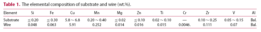
In order to generate a dataset for analysing and predicting optimal process parameters, WAAM experiments were performed using a Trans Plus Synergic 4000 CMT welder, VR1500 4R/F++ROBOTER wire feeder, KUKA six-axis robot, and protective gas device, as shown in Figure 1. The WAAM samples were produced on 2219 substrates (100 × 40 × 10 mm) by depositing ER2319 aluminium alloy wire with a diameter of 1.2 mm. Table 1 provides the chemical compositions of both substrates and filling materials. Argon gas with 99.99% purity was used for local protection to prevent impurity gas from entering the molten pool and producing material oxidation or increased porosity. It was coaxially outputted through the welding gun, maintaining a flow rate of 23 L/min.

Figure 1

Schematic diagram of the WAAM system.

Table 1

The elemental composition of substrate and wire (wt.%).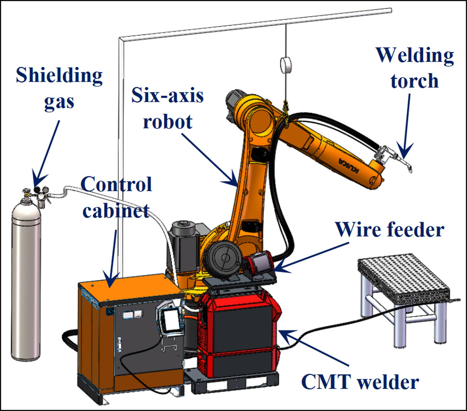

Element	Si	Fe	Cu	Mn	Mg	Zn	Ti	Cr	Zr	V	Al
Substrate	≤0.20	≤0.30	5.8∼6.8	0.20∼0.40	≤0.02	≤0.10	0.02∼0.10	—	0.10∼0.25	0.05∼0.15	Bal.
Wire	0.048	0.063	5.91	0.252	0.014	0.016	0.015	0.0046.	0.111	0.07	Bal.

Data collection and processing

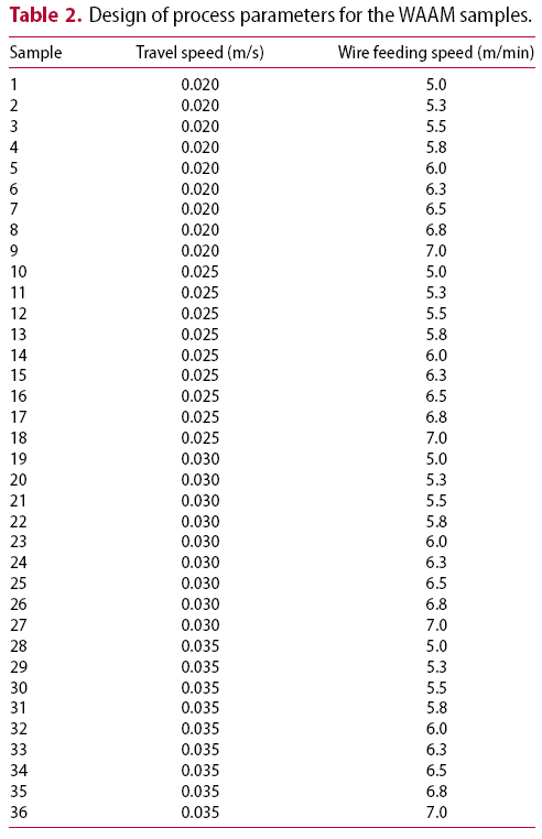
To characterise the influence of the primary process parameters of WAAM on grain morphology, porosity and tensile strength, full process parameters were presented in Table 2. Consequently, there were 36 test cases for three different amounts of layers, resulting in a total of 108 data points as potential inputs for the machine-learning algorithm.

Table 2

Design of process parameters for the WAAM samples.

Sample	Travel speed (m/s)	Wire feeding speed (m/min)
1	0.020	5.0
2	0.020	5.3
3	0.020	5.5
4	0.020	5.8
5	0.020	6.0
6	0.020	6.3
7	0.020	6.5
8	0.020	6.8
9	0.020	7.0
10	0.025	5.0
11	0.025	5.3
12	0.025	5.5
13	0.025	5.8
14	0.025	6.0
15	0.025	6.3
16	0.025	6.5
17	0.025	6.8
18	0.025	7.0
19	0.030	5.0
20	0.030	5.3
21	0.030	5.5
22	0.030	5.8
23	0.030	6.0
24	0.030	6.3
25	0.030	6.5
26	0.030	6.8
27	0.030	7.0
28	0.035	5.0
29	0.035	5.3
30	0.035	5.5
31	0.035	5.8
32	0.035	6.0
33	0.035	6.3
34	0.035	6.5
35	0.035	6.8
36	0.035	7.0

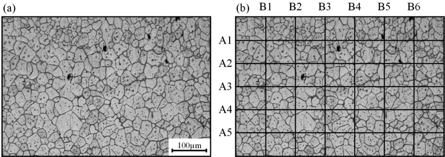
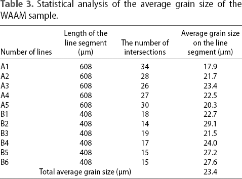
The ‘intercept method’ was used to measure and statistically analyse the grain size in the WAAM samples. The line segments were drawn at a uniform interval on the grain morphology diagram in Figure 2(a). The average grain size (d_ave) of the WAAM sample is defined as follows [34]:

d_{ave} = \frac{l}{i}

(1)

where l is the length of the line segment, i is the number of intersections between the line segment and grain boundaries. The data of average grain size obtained from all line segments drawn on the grain morphology diagram are presented in Table 3, corresponding to Figure 2(b). The upper, middle, and lower positions of each WAAM sample were chosen to produce accurate statistical outcomes. Additionally, five distinct microstructure regions at each aforementioned position were analysed to enhance the accuracy of the results further.

Figure 2

Statistical method for the grain size of WAAM 2319 alloy. (a) Grain morphology; (b) statistical method of average grain size.

Table 3

Statistical analysis of the average grain size of the WAAM sample.

Number of lines	Length of the line segment (µm)	The number of intersections	Average grain size on the line segment (µm)
A1	608	34	17.9
A2	608	28	21.7
A3	608	26	23.4
A4	608	27	22.5
A5	608	30	20.3
B1	408	18	22.7
B2	408	14	29.1
B3	408	19	21.5
B4	408	17	24.0
B5	408	15	27.2
B6	408	15	27.6
Total average grain size (µm)			23.4

The microstructure of WAAM samples was observed under various process parameters and positions, as shown in Figure 3(a). In order to enhance the visibility of the black pore morphology, the metallographic images were subjected to denoising, as demonstrated in Figure 3(b). The processed image was imported into Image-Pro Plus 6.0 software, and the pore morphology was marked in red to calculate the number and area of the pores in Figure 3(c,d). The porosity (P) of the WAAM samples is defined as [35]

P = \frac{\sum S_{i}}{S} \times 100 %

(2)

where

\sum S_{i}

is the sum of the areas of all pores in the metallographic diagram, S is the area of the metallographic diagram. Six different regions were taken from each WAAM sample to minimise measurement errors, and the porosity of each region was calculated using Equation (2).

Figure 3

Statistical method for the porosity of WAAM 2319 alloy. (a) Pore morphology; (b) noise reduction processing for images; (c) pore morphology marking; (d) calculation of porosity.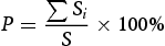

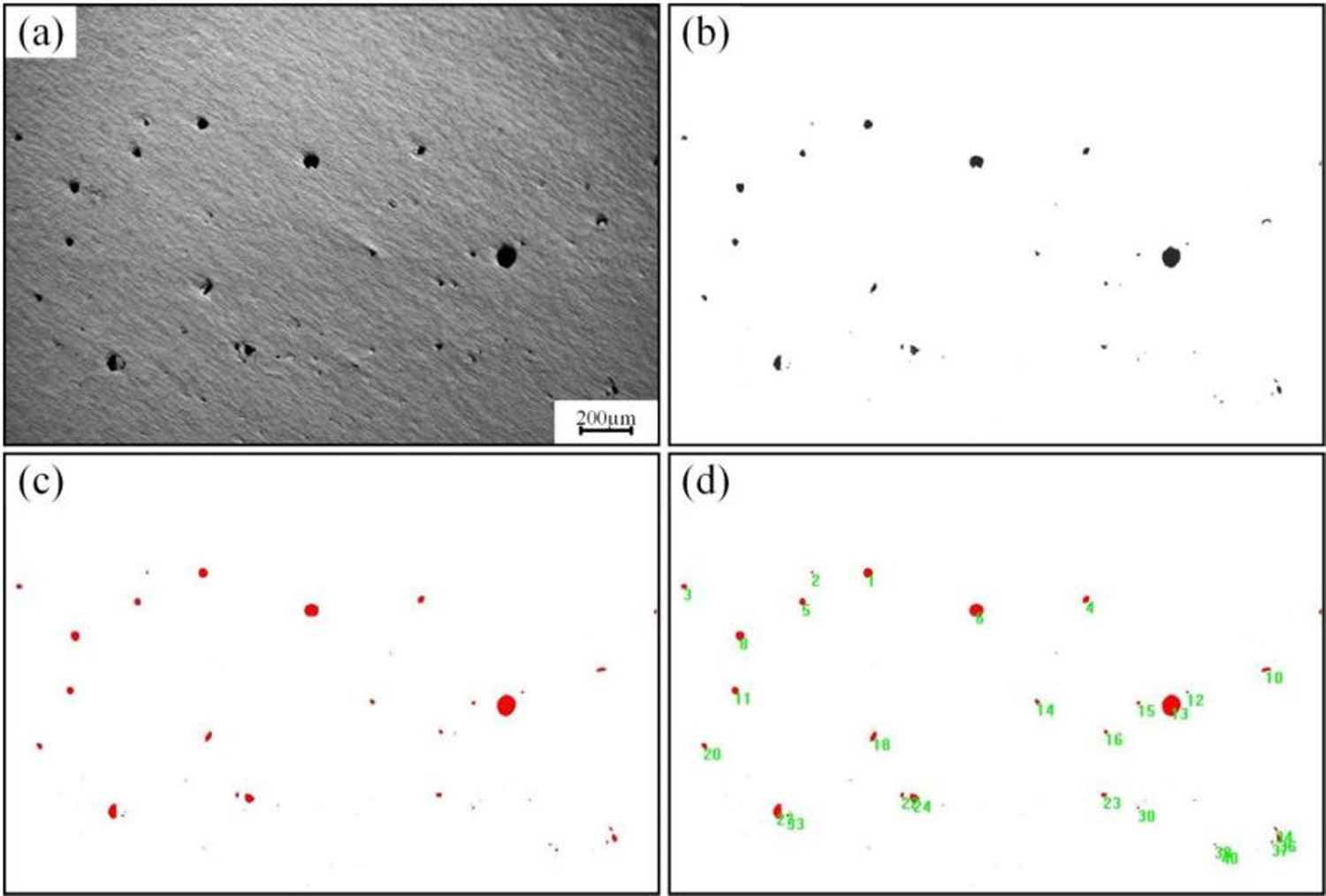
The tensile samples along both the deposition and scanning directions were cut by wire-cut electrical discharge machining (WEDM), as shown in Figure 4. Three tensile specimens were obtained in each direction to minimise possible experimental errors, and its average value was calculated. The loading speed was maintained at a constant rate of 1.0 mm/min during the entire tensile process. As a result, the grain size, porosity, and tensile strength of each WAAM sample for various process parameters were obtained to provide a data foundation for training models.

Figure 4

Schematic diagram of selection direction and dimensions of the tensile sample. (a) The position of tensile specimens in the WAAM block; (b) the size of the tensile specimens.

Neural network framework establishment

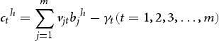
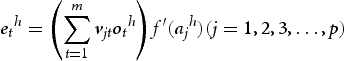
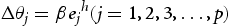
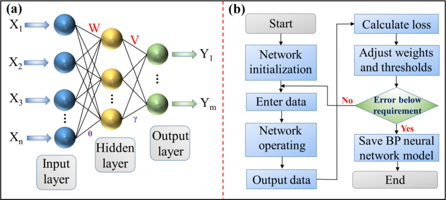
The usage of ANNs has become increasingly ubiquitous, with currently over 40 distinct network models available. Among these models, the Back Propagation (BP) neural network is widely adopted in engineering applications due to its straightforward architecture, robust computational ability, and superior generalisation capacity. The schematic illustration of the BP neural network architecture is presented in Figure 5(a). The sigmoid function is selected as the activation function in this BP neural network model. The function expression is given as [36]:

f (a) = \frac{1}{1 + e^{- k a}}

(3)

where k is the slope. when k tends to infinity, the Sigmoid function will be transformed into a Step function that can only take 1 or 0. Regarding the learning algorithm of the BP neural network, the definition of various variables is necessary [37,38]. The input data is given as follows:

X^{h} = ({x_{1}}^{h}, {x_{2}}^{h}, \dots, {x_{i}}^{h}, \dots, {x_{n}}^{h})^{T} (h = 1, 2, 3, \dots, k)

(4)

where n is the dimension of the input data, and h is the length of each dimension. The expected output data is given as follows:

Y^{h} = ({y_{1}}^{h}, {y_{2}}^{h}, \dots, {y_{i}}^{h}, \dots, {y_{m}}^{h})^{T} (h = 1, 2, 3, \dots, k)

(5)

where m is the dimension of the output data, and h is the length of each dimension corresponding to the input data. The net input data and net output data of the hidden layer are:

\begin{aligned} A^{h} & = ({a_{1}}^{h}, {a_{2}}^{h}, {a_{3}}^{h}, \dots, {a_{p}}^{h})^{T} (h = 1, 2, 3, \dots, k) \end{aligned}

(6)

\begin{aligned} B^{h} & = ({b_{1}}^{h}, {b_{2}}^{h}, {b_{3}}^{h}, \dots, {b_{p}}^{h})^{T} (h = 1, 2, 3, \dots, k) \end{aligned}

(7)

where p is the dimension of the input and output data of the hidden layer. The net input data and actual output data of the output layer are:

\begin{aligned} C^{h} & = ({c_{1}}^{h}, {c_{2}}^{h}, {c_{3}}^{h}, \dots, {c_{q}}^{h})^{T} (h = 1, 2, 3, \dots, k) \end{aligned}

(8)

\begin{aligned} D^{h} & = ({d_{1}}^{h}, {d_{2}}^{h}, {d_{3}}^{h}, \dots, {d_{q}}^{h})^{T} (h = 1, 2, 3, \dots, k) \end{aligned}

(9)

where q is the dimension of the net input data and actual output data of the output layer, corresponding to the dimension of the expected output data. The connection weights between the input layer and the hidden layer, as well as those between the hidden layer and the output layer, can be expressed as:

\begin{aligned} W & = {w_{i j}} (i = 1, 2, 3, \dots, n), (j = 1, 2, 3, \dots, p) \end{aligned}

(10)

\begin{aligned} V & = {v_{i j}} (j = 1, 2, 3, \dots, p), (t = 1, 2, 3, \dots, m) \end{aligned}

(11)

The thresholds for each unit in the hidden layer and output layer are:

\begin{aligned} θ & = {θ_{i j}} (j = 1, 2, 3, \dots, p) \end{aligned}

(12)

\begin{aligned} γ & = {γ_{i j}} (t = 1, 2, 3, \dots, m) \end{aligned}

(13)

Afterwards, the neural network model requires initialisation. The weights W and V and the thresholds θ and γ should be assigned random values between the intervals of [−1, 1]. A learning mode is also provided with random input and expected output data. The net input and output data expressions of the hidden layer are:

\begin{aligned} {a_{j}}^{h} & = \sum_{i = 1}^{n} w_{i j} {x_{i}}^{h} - θ_{j} (j = 1, 2, 3, \dots, p) \end{aligned}

(14)

\begin{aligned} {b_{j}}^{h} & = f ({a_{j}}^{h}) (j = 1, 2, 3, \dots, p) \end{aligned}

(15)

The net input and actual output data of the output layer can be expressed as:

\begin{aligned} {c_{t}}^{h} & = \sum_{j = 1}^{m} v_{j t} {b_{j}}^{h} - γ_{t} (t = 1, 2, 3, \dots, m) \end{aligned}

(16)

\begin{aligned} {d_{t}}^{h} & = f ({c_{t}}^{h}) (t = 1, 2, 3, \dots, m) \end{aligned}

(17)

Compared to the expected output, the error expressions for the output layer and the hidden layer are:

\begin{aligned} {o_{t}}^{h} & = ({y_{t}}^{h} - {d_{t}}^{h}) f^{'} ({c_{t}}^{h}) (t = 1, 2, 3, \dots, m) \end{aligned}

(18)

\begin{aligned} {e_{t}}^{h} & = (\sum_{t = 1}^{m} v_{j t} {o_{t}}^{h}) f^{'} ({a_{j}}^{h}) (j = 1, 2, 3, \dots, p) \end{aligned}

(19)

The learning rate is defined as α, and that value lies within the interval (0,1). The weight values from the hidden layer to the output layer and the correction factor for the thresholds of the output layer neurons can be expressed as follows:

\begin{aligned} Δ v_{j t} & = α {o_{t}}^{h} {b_{j}}^{h} (j = 1, 2, 3, \dots, p), (t = 1, 2, 3, \dots, m) \end{aligned}

(20)

\begin{aligned} Δ γ_{t} & = α {o_{t}}^{h} {b_{j}}^{h} (t = 1, 2, 3, \dots, m) \end{aligned}

(21)

Another learning rate β is defined with a value between (0,1). The weight values from the input layer to the hidden layer and the correction factor for the thresholds of the hidden layer neurons can be expressed as follows:

\begin{aligned} Δ w_{i j} & = β {e_{j}}^{h} {x_{i}}^{h} (i = 1, 2, 3, \dots, n), (j = 1, 2, 3, \dots, p) \end{aligned}

(22)

\begin{aligned} Δ θ_{j} & = β {e_{j}}^{h} (j = 1, 2, 3, \dots, p) \end{aligned}

(23)

The input and expected output data were calculated using the above formula until the final error reaching the desired level of accuracy. The operational framework of the BP neural network model was illustrated in Figure 5(b).

Figure 5

Establishment of BP neural network framework. (a) Schematic diagram of BP neural network structure; (b) BP neural network model operation process.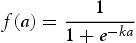

Result and discussion

Training and validation of forward models

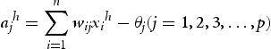
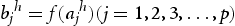
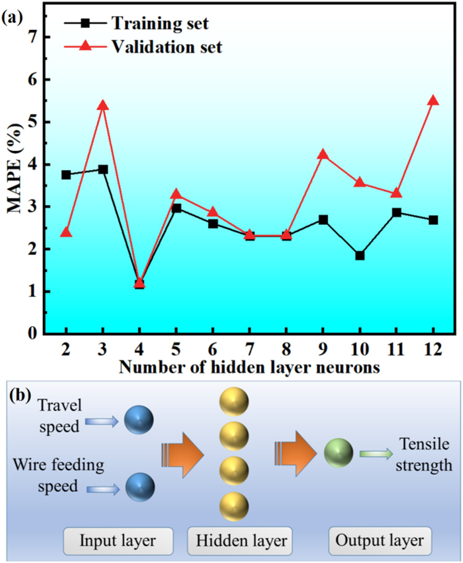
The input layer of the forward model consists of two neurons representing process parameters, including travel speed and wire feeding speed. The output layer produces the average tensile strength value of the WAAM sample. The optimal value for the number of hidden layer neurons is given as follows [39,40]:

p = \sqrt{n + m} + α

(24)

where p is the number of neurons in the hidden layer, n and m are the numbers of neurons in the input and output layers, respectively. α is the constant changing from 0 to 10. Therefore, it can be deduced from the formula (23) that the number of neurons in the hidden layer may vary between 2 and 12. In order to ensure the quality of the network and select an appropriate number of hidden layer neurons, training and validation samples should be used to evaluate the performance of the forward model. By calculating the mean absolute percentage error (MAPE) between predicted data and actual data, the relationship between the error value and the number of neurons in the hidden layer can be explored. The optimal values within the hidden layer neurons range should be traversed to obtain the trend. The expression for MAPE is as follows [41]:

MAPE = \frac{100 %}{n} \sum_{i = 1}^{n} | \frac{{\hat{y}}_{i} - y_{i}}{y_{i}} |

(25)

where

{\hat{y}}_{i}

represents the predicted value of the model,

y_{i}

represents the true value, and n represents the number of samples.

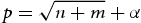
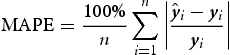
Figure 6(a) shows the MAPE values under different numbers of neurons in the hidden layer for the forward model. It is suggested that the error values for training samples in the forward model are generally lower than those for validation samples. When there are 3 neurons in the hidden layer, the prediction error of the training samples is relatively high, reaching 3.88%. However, as the number of neurons in the hidden layer increases, the prediction error for training samples stabilises at around 2.0%, with minor fluctuations. Meanwhile, the error value of the validation sample fluctuates significantly with changing the number of neurons in the hidden layer. When the number of neurons in the hidden layer is 6, errors for both datasets are relatively small, with an error of only 1.09% for the validation sample. Therefore, the forward model consists of two neurons in the input layer, six neurons in the hidden layer, and one neuron in the output layer, as shown in Figure 6(b).

Figure 6

BP forward model prediction. (a) The variation of MAPE value with the number of hidden layers in the training and validation sets; (b) structure diagram of BP forward network model.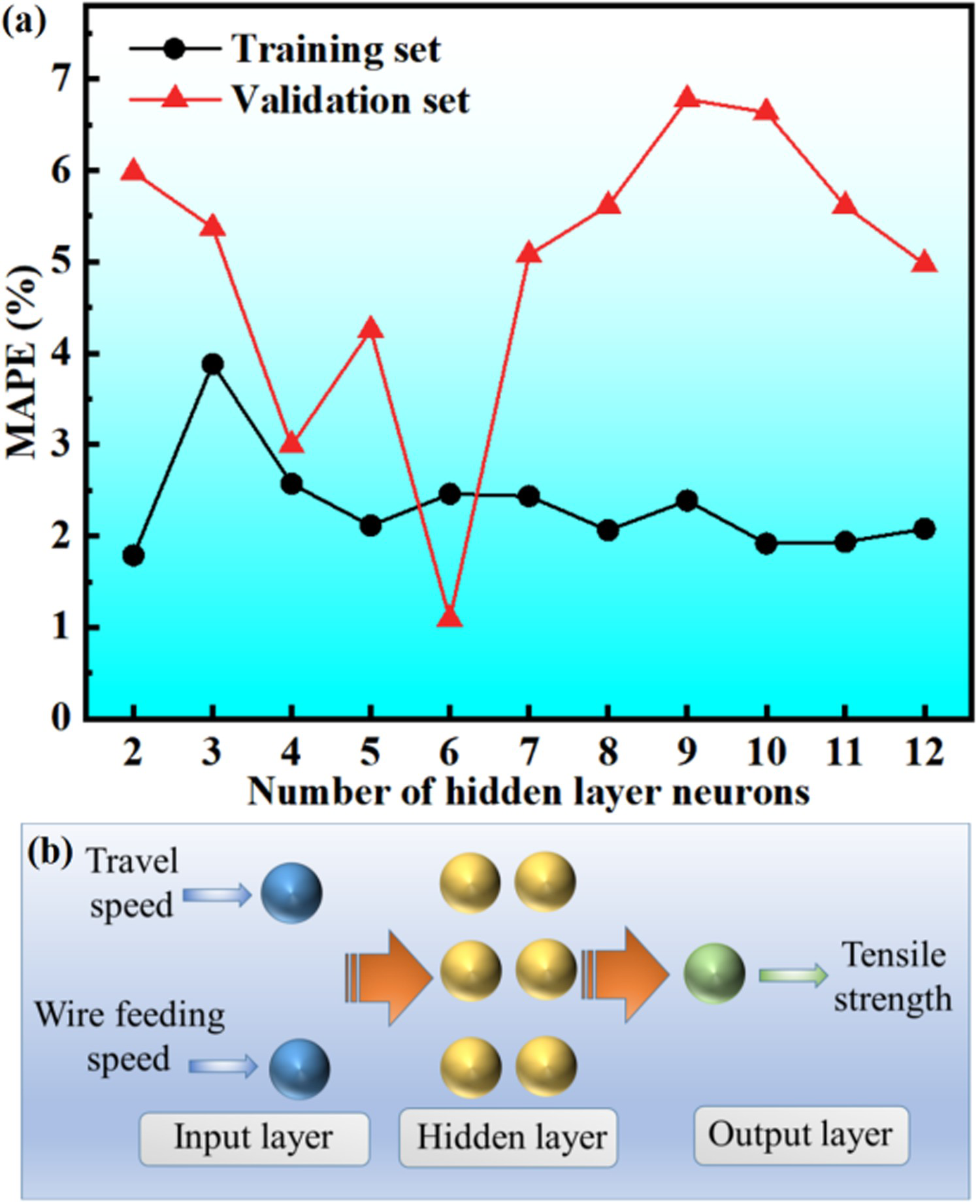

The 36 sets of process parameter data during the WAAM process are randomly divided into three groups, including 28 for the training set, 4 for the validation set, and 4 for the testing set. Figure 7 depicts the relationship between the mean square error (MSE) and the number of iterations during the training process of the forward model. The expression for MSE is as follows [39]:

MSE = \frac{1}{n} \sum_{i = 1}^{n} {({\hat{y}}_{i} - y_{i})}^{2}

(26)

where

{\hat{y}}_{i}

represents the predicted value of the model,

y_{i}

represents the true value, and n represents the number of samples.

Figure 7

The performance of the training process for the BP forward model.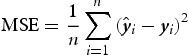

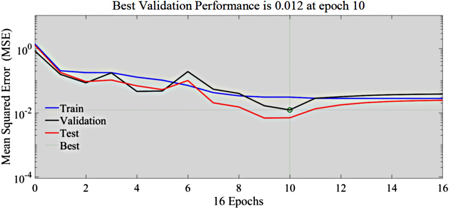
The blue, green, and red curves in the plot demonstrate the variation of the MSE with the number of iterations of the training set, validation set, and test set in the BP forward model prediction in Figure 7. The generalisation ability of the current model can be observed through the validation set curve. Meanwhile, the testing set curve allows for an assessment of the generalisation ability of the final application in this model. As the number of iterations increases, this graph shows a decreasing trend in the MSE of each dataset. The circle in the plot denotes the position of the minimum error value predicted by the validation set. It can be inferred that the BP neural network undergoes 16 iterations of training and the lowest MSE of 0.012 in the 10th iteration is attained. The final error value tended to stabilise, which indicated that the BP forward model could establish an optimal mapping relationship between process parameters and mechanical properties.

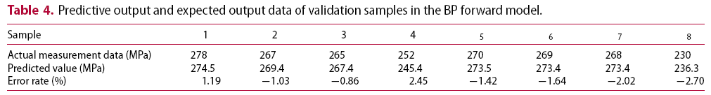
The trained BP forward model is utilised to input the training and validation samples separately to obtain predicted tensile strength results. These predicted outputs are subsequently compared against the actual tensile strength values, as depicted in Figure 8(a,b). Figure 8(a) displays the close consistency between the predicted output and the expected output, with a controlled deviation at approximately 1%, demonstrating that the BP mentioned above neural network model is highly accurate. Additionally, Figure 8(b) compares the predicted and expected output values of the validation samples. Compared to the fitting results for the training samples, prediction accuracy for the validation samples has slightly decreased, with specific values listed in Table 4. Samples 4, 7, and 8 show the highest relative prediction errors, with error rates of 2.45%, −2.02% and −2.70%, respectively. In contrast, the absolute values of other respective error rates remain under 2.0%.

Figure 8

Comparison of predicted output results with the expected output results of the BP forward model. (a) Predictive output and expected output results of training samples; (b) predictive output and expected output results of validation samples.

Table 4

Predictive output and expected output data of validation samples in the BP forward model.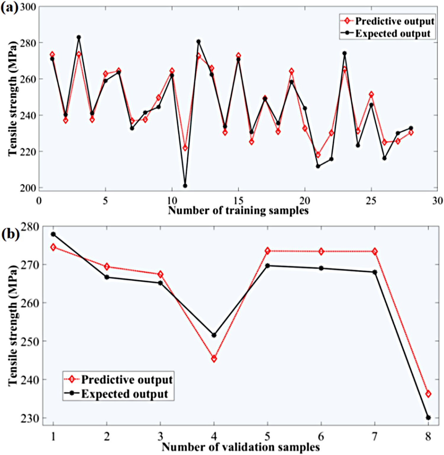

Sample	1	2	3	4	₅	₆	₇	₈
Actual measurement data (MPa)	278	267	265	252	270	269	268	230
Predicted value (MPa)	274.5	269.4	267.4	245.4	273.5	273.4	273.4	236.3
Error rate (%)	1.19	−1.03	−0.86	2.45	−1.42	−1.64	−2.02	−2.70

Genetic algorithm optimisation of BP neural network

The genetic algorithm uses real number encoding, where each string comprises the connection weights between the input layer and hidden layer, the threshold of the hidden layer, the connection weights between the hidden layer and output layer, and the threshold of the output layer. The fitness value F is given as [41]:

F = k (\sum_{i = 1}^{n} abs (y_{i} - d_{i}))

(27)

where n is the number of output nodes in the network, y_i denotes the predicted output of the ith node, and d_i represents the actual output value of the ith node. The genetic algorithm is applied to optimise the previously established BP forward model. The model parameters are set as follows: population size is 10, number of evolutions is 50, crossover probability is 0.4 and mutation probability is 0.2. Figure 9(a) shows the MAPE values of the training and validation samples calculated within the range of [2,12] neurons in the hidden layer. When the number of neurons in the hidden layer was set to 4, the errors of both the training and validation samples were minimised, with values of 1.17% and 1.18%, respectively. Therefore, the GA-BP forward model consists of two neurons in the input layer, four neurons in the hidden layer and one neuron in the output layer, as shown in Figure 9(b).

Figure 9

GA-BP forward model prediction. (a) The variation of MAPE value with the number of hidden layers in the training and validation sets; (b) the forward network model structure diagram.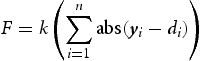

All the sample data is randomly partitioned into 28 training sets, 4 validation sets, and 4 testing sets. Figure 10 illustrates the variation in MSE with the number of iterations during the training process of the GA-BP forward model. It can be observed that the GA-BP forward model achieved the minimum MSE value (0.004) at the 9th iteration and reached convergence after 15 training sessions. Compared to the BP forward model, the GA-BP forward model exhibited a one-order-of-magnitude reduction in MSE, indicating significantly improved prediction accuracy.

Figure 10

The performance of the training process for the BP forward model.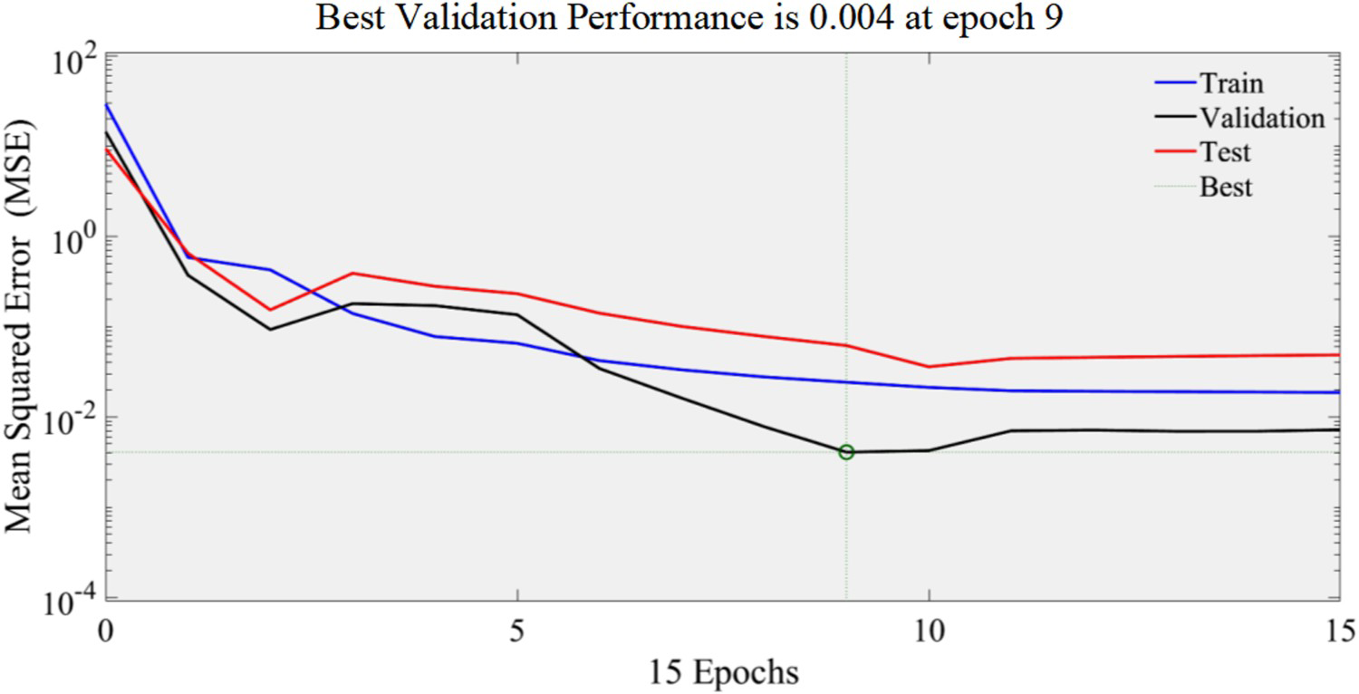

Figure 11 depicts the regression analysis of the training, validation, and test sets during the training process of the GA-BP forward model. The vertical and horizontal axes of this figure represent predicted and expected values, respectively. A complete fit is indicated when the curve falls on the diagonal with a regression value of 1. The correlation coefficient between predicted and expected outputs was 0.96 for the validation set and 0.99 for the test set. An overall regression reach 0.97 for the sample, which illustrated that the GA-BP forward model produced excellent training results.

Figure 11

Regression analysis diagram of the training process of the GA-BP forward model. (a) Regression analysis of training set; (b) regression analysis of validation set; (c) regression analysis of test set; (d) an overall regression of samples.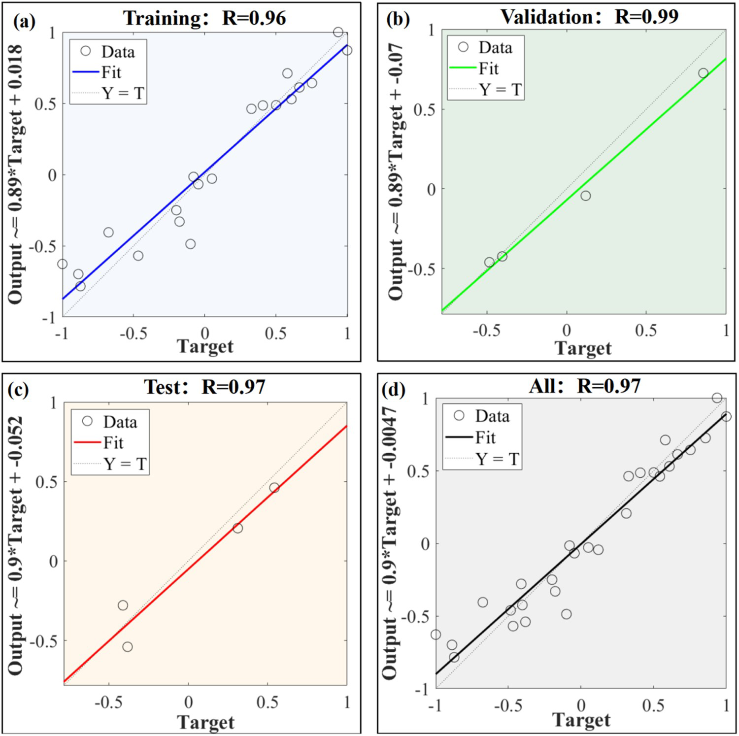

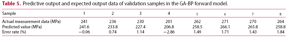
After inputting the training samples into the GA-BP forward model, the predicted and expected output results are shown in Figure 12(a). Except for a slight deviation between samples 19 and 24, the predictions of the remaining samples are consistent with the expected output results. Figure 12(b) presents the predicted and expected output results of the validation sample in the GA-BP forward model, and the specific values are listed in Table 5. Sample 4 has the highest prediction error rate at −2.86%, while the error rates of the other samples are all less than 2.0%. These results indicate that the training effect of the GA-BP forward model is excellent.

Figure 12

Comparison of predicted output results with expected output results in the GA-BP forward model. (a) Predictive output and expected output results of training samples; (b) predictive output and expected output results of validation samples.

Table 5

Predictive output and expected output data of validation samples in the GA-BP forward model.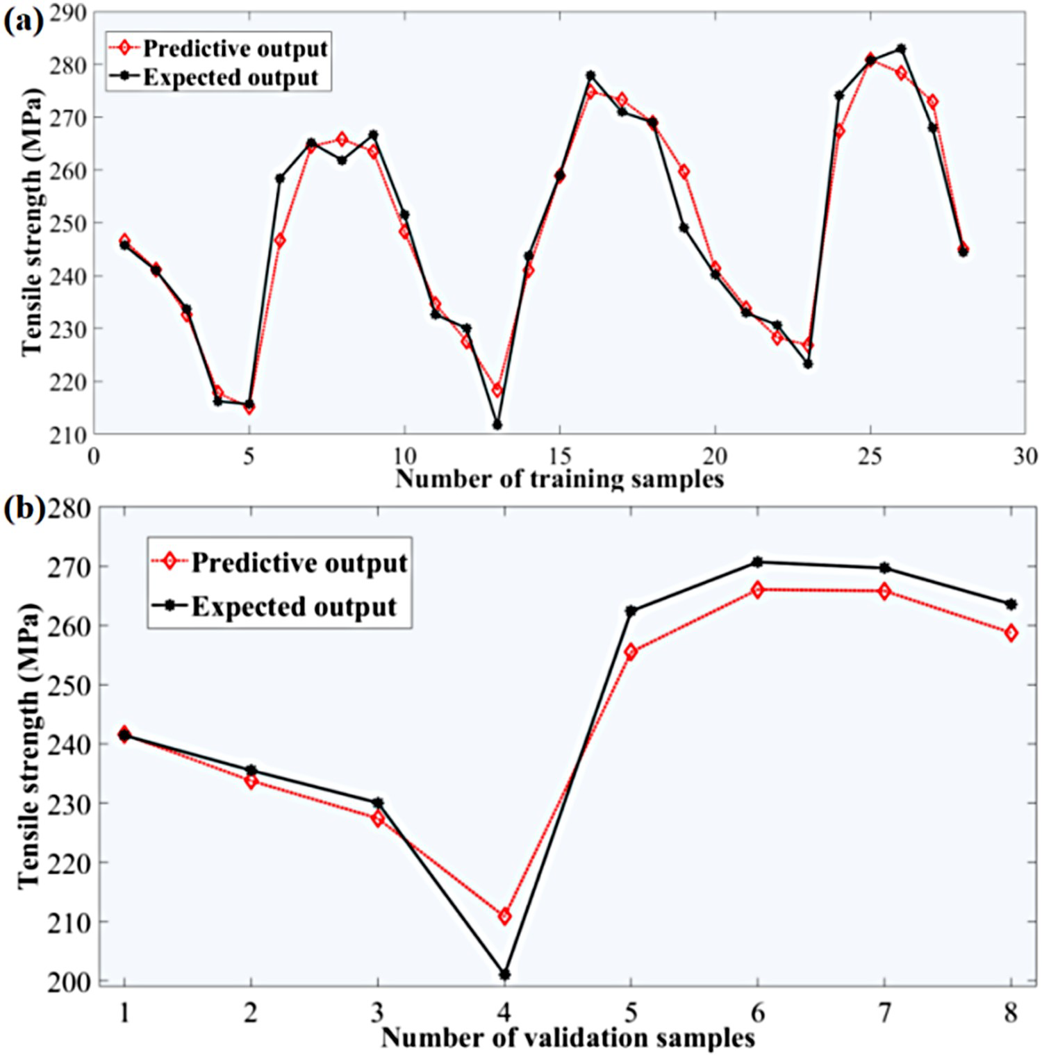

Sample	1	2	3	4	₅	₆	₇	₈
Actual measurement data (MPa)	241	236	230	201	262	271	270	264
Predicted value (MPa)	241.6	233.8	227.4	206.8	258.5	266.1	265.8	258.8
Error rate (%)	−0.06	0.74	1.14	−2.86	1.49	1.71	1.43	1.84

The joint design of forward and reverse models for WAAM 2319 alloy

The GA-BP forward model exhibits high accuracy and provides results consistent with actual tensile strength outcomes. Therefore, additional process parameter combinations are obtained as WAAM sample datasets through the GA-BP forward model to train the corresponding GA-BP reverse model.

In the above sections, 36 sets of tensile strength datasets are obtained through the WAAM experiments under different process parameter combinations. The travel speed range for input layer prediction within the GA-BP forward model was 0.020–0.030 m/s, while the wire feeding range was 5.0–7.0 m/min. When a travel speed gradient is 0.001 m/s and a wire feeding speed gradient is 0.1 m/min, it is possible to obtain 24 process parameters, which consist of 12 travel speed parameters and 12 wire feeding speed parameters. A total of 16 parameters are utilised in calculating the travel speed, including 4 parameters derived from experimental testing and an additional 12 parameters obtained from the GA-BP forward model. Similarly, a total of 21 parameters are utilised to calculate the wire feeding speed. There are 9 parameters gathered through experimental results, while the remaining 12 are derived from the GA-BP forward model. Finally, 336 process parameter combinations are obtained, including 36 experimental data points and an additional 300 data points predicted by the GA-BP forward model.

The designed 300 sets of parameter combinations are input into the pre-trained GA-BP forward model. The predicted tensile strength results are shown in Figure 13(a). The GA-BP reverse model consists of 1 neuron in the input layer, 10 neurons in the hidden layer and 2 neurons in the output layer, as shown in Figure 13(b).

Figure 13

Structure design and prediction of GA-BP reverse model. (a) Structure diagram of GA-BP reverse network model; (b) prediction of tensile strength results using GA-BP forward model.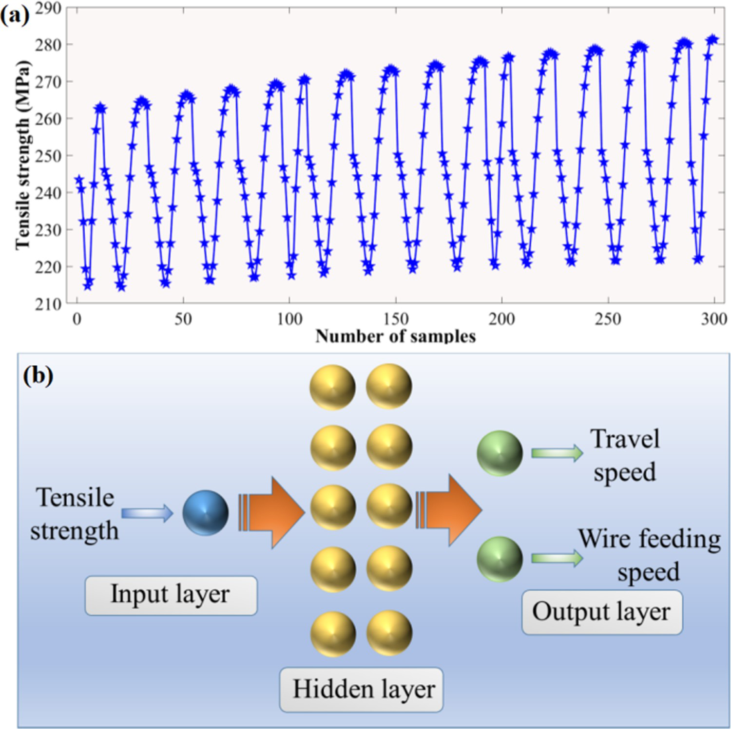

The predicted output results of the GA-BP reverse model for 16 groups of validation samples are listed in Table 6, with corresponding results graphically displayed in Figure 13. In predicting the travel speed, the 10th and 11th samples are close to the expected values, while there are some deviations in the rest samples. Among them, the 9th sample has the largest deviation (an error rate of 23.89%), with an average error of 1.55%, as shown in Figure 13(a). The error rate of the wire feeding speed is generally low, with an average error of 3.1%. The 12th sample has the highest error rate, reaching 6.56%, as shown in Figure 13(b).

Table 6

Comparison of predicted output and expected output of GA-BP reverse engineering model validation samples.

Sample	Actual value of travel speed (m/s)	Prediction value of travel speed (m/s)	Error rate (%)	Actual value of wire feeding speed (m/min)	Prediction value of wire feeding speed (m/min)	Error rate (%)
1	0.034	0.0279	−17.81	5.3	5.62	6.08
2	0.024	0.0262	9.18	6.6	6.65	0.70
3	0.024	0.0247	3.07	6.4	6.60	3.08
4	0.025	0.0279	11.54	6.2	6.01	−3.06
5	0.031	0.0291	−6.03	5.7	5.67	−0.56
6	0.029	0.0279	−3.66	5.8	5.70	−1.78
7	0.031	0.0295	−4.96	5.1	5.33	4.47
8	0.029	0.0303	4.49	6.9	6.70	−3.00
9	0.020	0.0248	23.89	6.8	6.65	−2.15
10	0.033	0.0331	0.37	6.7	6.77	0.99
11	0.033	0.0327	−0.86	7	6.75	−3.53
12	0.024	0.0275	14.41	5	5.33	6.56
13	0.030	0.0288	−4.03	5.9	5.60	−5.06
14	0.028	0.0295	5.42	6.9	6.68	−3.19
15	0.025	0.0279	11.51	5	5.17	3.31
16	0.033	0.0259	−21.66	5.3	5.41	2.08

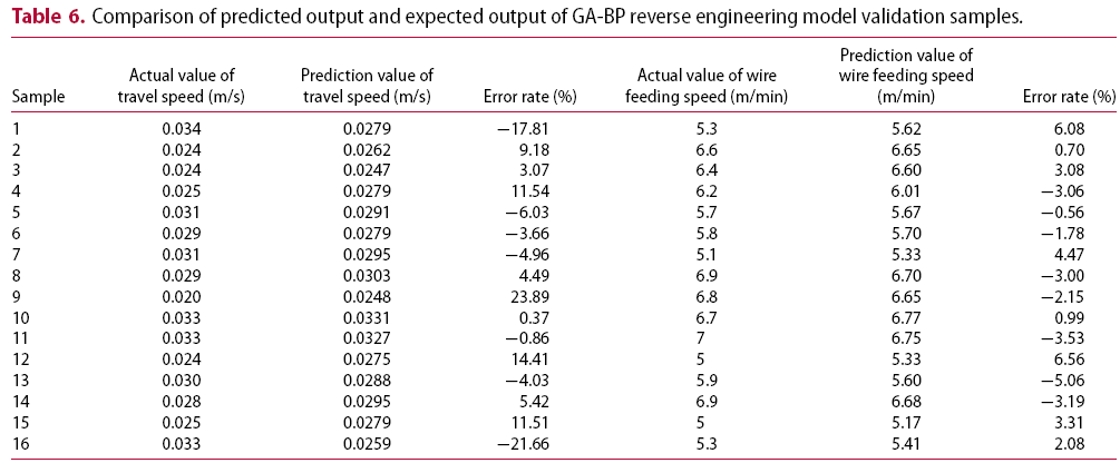
In summary, it can be considered that the GA-BP reverse model is more accurate in predicting the wire feeding speed and meeting user needs. To further improve the overall prediction accuracy of the reverse model, the GA-BP forward model was added as a criterion in the design of the reverse model. The final prediction output flowchart of the reverse model is shown in Figure 14(c). The target tensile strength value should be input into the reverse model to predict the corresponding travel speed and wire feeding speed by utilising the GA-BP model. Then the acquired predicted process parameters are input into the GA-BP forward model to gain further clarity into achievable tensile strength values under these designated process parameters. After that, an evaluation must determine if the obtained tensile strength value aligns with the required accuracy ranges. The process parameter design plan will be output directly if requirements are met. Conversely, if requirements are not fulfilled, the travel speed can be changed while maintaining a fixed wire feeding speed until satisfactory outcomes are achieved using the GA-BP forward model.

Figure 14

Predicted output and expected output of process parameters in the GA-BP reverse model. (a) Comparison of predicted output and expected output of GA-BP reverse model for travel speed; (b) comparison between the predicted output and expected output of the GA-BP reverse model for wire feeding speed.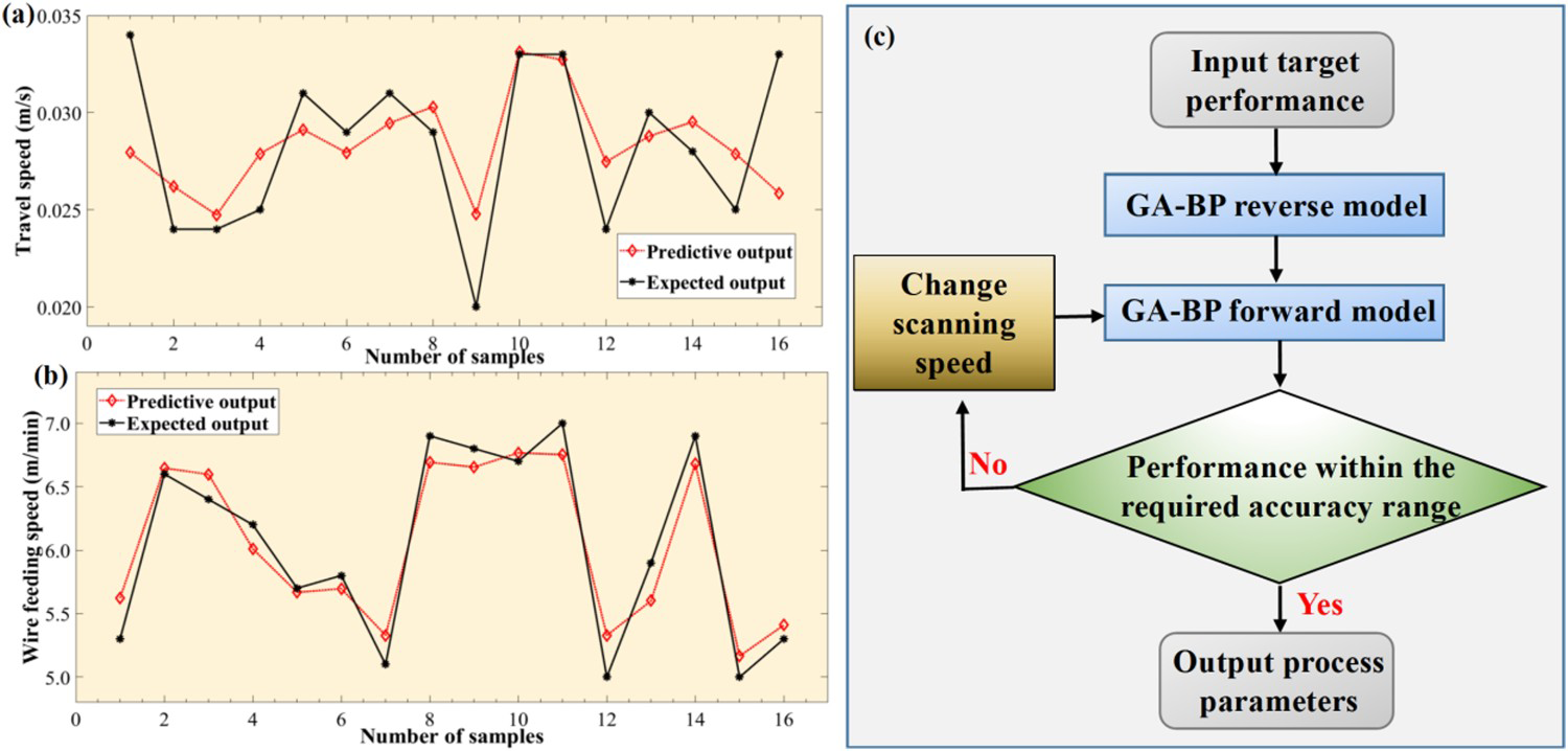

Verification of process parameter reverse design result for WAAM 2319 alloy

Based on the mechanical performance requirements of WAAM 2319 alloy components, multiple process parameter combination schemes are designed using the reverse model described in Section 3.2. With the objective of manufactruing WAAM 2319 alloy samples with tensile strength values not less than 230 MPa, a sequence of 11 evenly spaced datasets ranging from 230 to 280 MPa were suitable input parameters for execution of the reverse model for effective process parameter design. The output of multiple sets of process parameter combinations may be achieved through the GA-BP reverse model. Coupled with the GA-BP forward model, accurate prediction is achieved concerning the tensile strength values of WAAM components under diverse process parameter configurations. Ultimately, process parameters with corresponding predicted tensile strengths not less than 230 MPa will be identified as suitable output results.

In order to validate the predictive accuracy of our reverse model, two sets of parameter combinations for curvilinear component printing from among multiple process parameters are chosen. The first set maintains a travel speed of 0.030 m/s and a wire feeding speed of 5.9 m/min (Component 1), while the travel speed and wire feeding speed are set to 0.028 m/s and 6.9 m/min (Component 2) in the second set, respectively. Figure 15 shows the curved components manufactured and designed by the reverse model. From the top view, it can be seen that the collapse phenomenon at both ends of Component 2 is obvious, and the side surface is relatively rough compared to Component 1. From the front view, the top contour of Component 1 is approximately a straight line, while both ends of its curved components are about 12 mm lower than the middle position.

Figure 15

Physical drawing of curved components. (a) The vertical view of Component 1; (b) the vertical view of Component 2; (c) the front view of Component 1; (d) the front view of Component 2.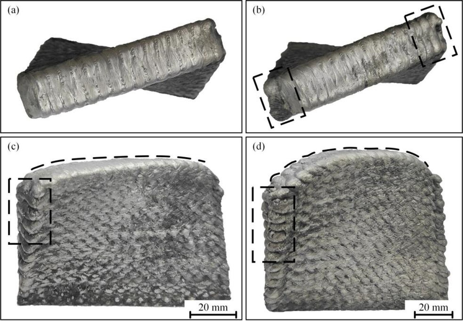

In addition, three groups of tensile samples are made on the same WAAM block to avoid the contingency of tensile results. The fracture position and average tensile strength of samples are shown in Figure 16. It can be found that the tensile strength of the components exceeds 230 MPa, which meets the mechanical performance design requirements. After inputting the two sets mentioned above of process parameters into the GA-BP forward model, Table 7 accurately portrays their predicted outcomes. It demonstrates that the maximum prediction error rate of the GA-BP forward model is 3.24%. The external environmental instability, irregularities in the preparation of tensile specimens, and variations in clamping angles are contributed to deviations in mechanical performance results. Therefore, a reverse model with a predictive accuracy rate below 6.0% should still be deemed satisfactory.

Figure 16

The fracture position and average tensile strength of samples.

Table 7

Predicting the tensile strength value of the WAAM components through the forward model.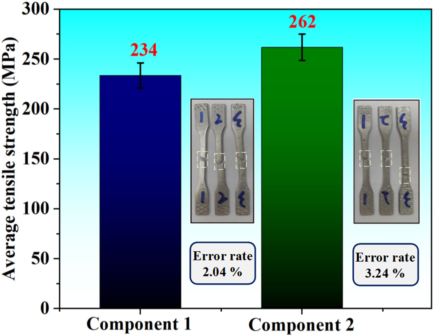

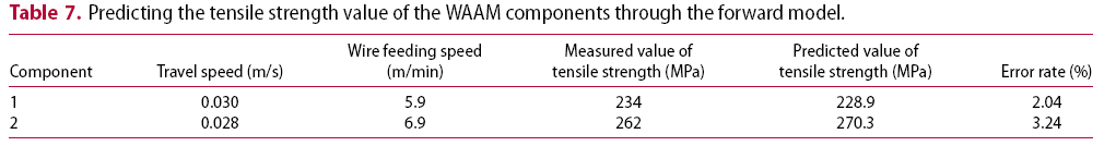
Component	Travel speed (m/s)	Wire feeding speed (m/min)	Measured value of tensile strength (MPa)	Predicted value of tensile strength (MPa)	Error rate (%)
1	0.030	5.9	234	228.9	2.04
2	0.028	6.9	262	270.3	3.24

Figure 17 shows the microstructure morphology of curved components at different positions. It can be found that the bottom and middle of component 1 are mainly composed of equiaxed grains with varying grain sizes, as shown in Figure 17(a,b). The equiaxed dendrites are mainly present at the top of component 1 in Figure 17(c). Figure 17(d–f) depicts variances in the microstructure morphology of curved component 2, consistent with patterns gleaned previously from Figure 17(a–c).

Figure 17

Microstructure of curved components produced by the WAAM process. (a) Microstructure in the bottom of Component 1; (b) microstructure in the middle of Component 1; (c) microstructure in the top of Component 1; (d) microstructure in the bottom of Component 2; (e) microstructure in the middle of Component 2; (f) microstructure in the top of Component 2.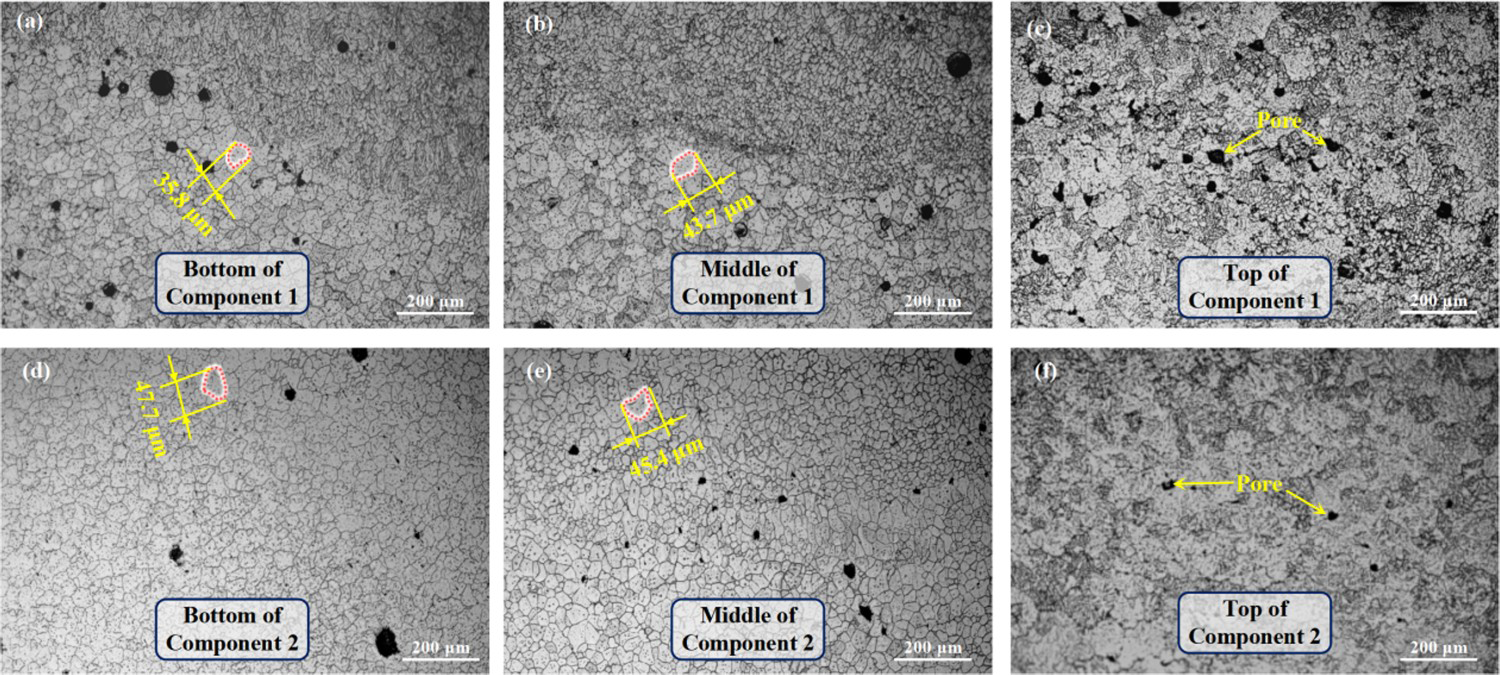

Average grain size values are calculated for both types of components’ bottom, middle, and top regions using the ‘intercept method’, as shown in Figure 18. It was discovered that comparatively coarse average grain sizes are presented in the middle and bottom regions of WAAM components under identical process parameters. In comparison to curved component 1, it is observed that component 2 exhibits a markedly larger grain size. Since the application of lower travel speeds and higher wire feeding speeds lead to enhance heat inputs during the WAAM process.

Figure 18

Statistics of average grain size and porosity of the WAAM components.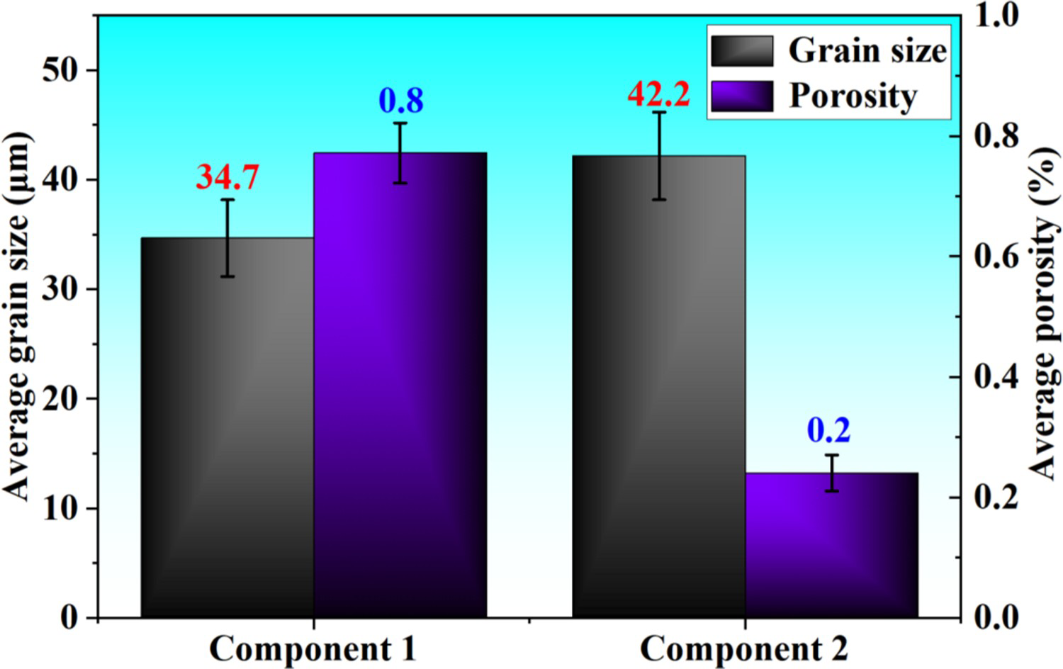

In addition, Figure 17 shows the distribution of pores in the WAAM component. It is suggested that pores are predominantly distributed around the interlayer area, and yellow dashed lines have been utilised to highlight this area. Component 2 has a smaller number and area of pores than component 1. The porosity of the WAAM sample goes decline with the decrease of travel speed and the increase of wire feeding speed in Figure 18. Therefore, component 2 has lower porosity and higher tensile strength values than that in component 1, which is consistent with the tensile strength predicted results of the above model.

Conclusion

This paper establishes the BP forward model based on conducted experiments. Then the BP forward model is integrated with the genetic algorithm to establish an optimal GA-BP model. As a result, this approach produces more accurate predictions of tensile strength for WAAM 2319 alloy. Finally, the output layer of the GA-BP forward model is trained as the input layer of the reverse model, which accurately predicts process parameter combinations. The main conclusions are obtained as follows:

This study constructs a BP forward model to establish the relationship between process parameters and tensile strength, and optimal model quality is achieved when using six hidden layer neurons. Through repeated iterative training, the error rates of the prediction performance for the BP forward model are all below 3.0%.

This study optimises the BP neural network by incorporating a genetic algorithm with a better global search capability. The GA-BP reverse model is developed, which exhibits promising prediction accuracy, with the MAPE value of 3.10% for predicting wire feeding speed and 1.55% for travel speed prediction.

This study uses a reverse model to design a combination of WAAM process parameters with a tensile strength higher than 230 MPa. Two sets of samples are selected for statistical analysis of their average grain size and porosity. The increase in grain size is attributed to the use of lower travel speed and higher wire feeding speed during the WAAM process, resulting in higher heat input. The porosity of the WAAM sample decreases with decreasing travel speed and increasing wire feeding speed resulting in a higher tensile strength value, which is consistent with the performance predictions generated by the GA-BP model.

The main process parameters in this study are travel speed and wire feeding speed. In the future, variables should be added to further explore the effects of process parameters such as interlayer cooling time, scanning path, and current mode on the WAAM parts, and they should be added to the process parameter database of the reverse engineering model for training [42].

Footnotes

Disclosure statement

No potential conflict of interest was reported by the author(s).

References

Armstrong

, Mehrabi

, Naveed

An overview of modern metal additive manufacturing technology. J Manuf Process. 2022;84:1001–1029. doi:10.1016/j.jmapro.2022.10.060

Zhan

, Wang

, . Regionalization of microstructure and mechanical properties of Ti6Al4V transition area fabricated by WAAM-LMD hybrid additive manufacturing. J Alloy Compd. 2022;929:167345. doi:10.1016/j.jallcom.2022.167345

Srivastava

, Rathee

, Tiwari

, . Wire arc additive manufacturing of metals: a review on processes, materials and their behaviour. Mater Chem Phys. 2023;294:126988. doi:10.1016/j.matchemphys.2022.126988

, Wang

, . Wire and arc additive manufacturing of lightweight metal components in aeronautics and astronautics. Aeronaut Manuf Technol. 2018;61:74–89.

Liu

, Xu

, Ge

, . Wire and arc additive manufacturing of metal components: a review of recent research developments. Int J Adv Manuf Tech. 2020;111:149–198. doi:10.1007/s00170-020-05966-8

, Tang

, Lu

, . Hot-wire arc additive manufacturing of aluminum alloy with reduced porosity and high deposition rate. Mater Des. 2021;199:109370. doi:10.1016/j.matdes.2020.109370

Bartsch

, Kühne

, Citarelli

, . Fatigue analysis of wire arc additive manufactured (3D printed) components with unmilled surface. Structures. 2021;31:576–589. doi:10.1016/j.istruc.2021.01.068

Qiu

, Dong

, Wu

, . Tailoring the surface finish, dendritic microstructure and mechanical properties of wire arc additively manufactured Hastelloy C276 alloy by magnetic arc oscillation. Addit Manuf. 2021;48:102397. doi:10.1016/j.addma.2021.102397

Palani

, Murugan

Optimization of weld bead geometry for stainless steel claddings deposited by FCAW. J Mater Process Tech. 2007;190:291–299. doi:10.1016/j.jmatprotec.2007.02.035

10.

Karaoğlu

, Seçgin

Sensitivity analysis of submerged arc welding process parameters. J Mater Process Tech. 2008;202:500–507. doi:10.1016/j.jmatprotec.2007.10.035

11.

Sondagar

, Bhadauria

, Sharma

Artificial neural network (ANN) based prediction of process parameters in additive manufacturing. IOP Conf Ser. 2021;1136:012026. doi:10.1088/1757-899X/1136/1/012026

12.

McCulloch

, Pitts

A logical calculus of the ideas immanent in nervous activity. B Math Biol. 1943;5:115–133.

13.

Shevchik

, Kenel

, Leinenbach

, . Acoustic emission for in situ quality monitoring in additive manufacturing using spectral convolutional neural networks. Addit Manuf. 2018;21:598–604. doi:10.1016/j.addma.2017.11.012

14.

Zhang

, Hong

, Ye

, . Extraction and evaluation of melt pool, plume and spatter information for powder-bed fusion AM process monitoring. Mater Des. 2018;156:458–469. doi:10.1016/j.matdes.2018.07.002

15.

Scime

, Beuth

A multi-scale convolutional neural network for autonomous anomaly detection and classification in a laser powder bed fusion additive manufacturing process. Addit Manuf. 2018;24:273–286. doi:10.1016/j.addma.2018.09.034

16.

Alhaddad

, He

, Halabi

, . Optimizing the material and printing parameters of the additively manufactured fiber-reinforced polymer composites using an artificial neural network model and artificial bee colony algorithm. Structures. 2022;46:1781–1795. doi:10.1016/j.istruc.2022.10.134

17.

Ling

, Ni

, Antonissen

, . Numerical prediction of microstructure and hardness for low carbon steel wire arc additive manufacturing components. Simul Model Pract Theory. 2023;122:102664. doi:10.1016/j.simpat.2022.102664

18.

Leirmo

, Martinsen

Evolutionary algorithms in additive manufacturing systems: discussion of future prospects. Procedia CIRP. 2019;81:671–676. doi:10.1016/j.procir.2019.03.174

19.

Joy

, Kuzhivelil

, Kannan

, . ANN modelling of additively manufactured carbon fibre integrated ABS. Mater Today. 2022;72:3137–3143. doi:10.1016/j.matpr.2022.10.004

20.

Patpatiya

, Shastri

, Sharma

, . ANN-predictive modeling and GA-optimization for minimizing dimensional tolerance in polyjet additive manufacturing. CIRP J Manuf Sci Technol. 2022;38:320–339. doi:10.1016/j.cirpj.2022.05.004

21.

Teharia

, Singari

, Kumar

Optimization of process variables for additive manufactured PLA based tensile specimen using taguchi design and artificial neural network (ANN) technique. Mater Today. 2021;56:3426–3432. doi:10.1016/j.matpr.2021.10.376

22.

, Zhang

, Wang

, . Deep learning based online metallic surface defect detection method for wire and arc additive manufacturing. Robot Comput Integr Manuf. 2023;80:102470. doi:10.1016/j.rcim.2022.102470

23.

, Lee

, Kim

Prediction of deposition bead geometry in wire arc additive manufacturing using machine learning. J Mater Res Technol. 2022;20:4283–4296. doi:10.1016/j.jmrt.2022.08.154

24.

Snell

, Sam

, Lova

, . Methods for rapid pore classification in metal additive manufacturing. JOM. 2020;72:101–109. doi:10.1007/s11837-019-03761-9

25.

Thompson

, Bian

, Shamsaei

, . An overview of direct laser deposition for additive manufacturing; part I: transport phenomena, modeling and diagnostics. Addit Manuf. 2015;8:36–62. doi:10.1016/j.addma.2015.07.001

26.

Fang

, Wang

, . Effect of reconstruction algorithm on the identification of 3D printing polymers based on hyperspectral CT technology combined with artificial neural network. Materials (Basel). 2020;13:1963. doi:10.3390/ma13081963

27.

Ahmadi

, Mirzaeifar

, Moghaddam

, . Effect of manufacturing parameters on mechanical properties of 316L stainless steel parts fabricated by selective laser melting: a computational framework. Mater Design. 2016;112:328–338. doi:10.1016/j.matdes.2016.09.043

28.

Chan

Modelling gas metal arc weld geometry using artificial neural network technology. Can Metall Quart. 1999;38:43–51.

29.

Kim

, Jong

, Park

, . A study on prediction of bead height in robotic arc welding using a neural network. J Mater Process Tech. 2002;130:229–234. doi:10.1016/S0924-0136(02)00803-8

30.

Geng

, Lin

, Wang

, . Modeling research of artificial neural networks of YAG laser welding parameters. Trans China Weld Inst. 2001;22:37–40.

31.

Xiong

, Zhang

, Hu

, . Optimizing of welding parameters of YAG laser welding titanium alloy based on artificial neural net. Appl Laser. 2001;21:243–246.

32.

Karmuhilan

, Anoop

Intelligent process model for bead geometry prediction in WAAM. Mater Today. 2018;5:24005–24013. doi:10.1016/j.matpr.2018.10.193

33.

Farias

, Filho

, Oliveira

Prediction of the interpass temperature of a wire arc additive manufactured wall: FEM simulations and artificial neural network. Addit Manuf. 2021;48:102387. doi:10.1016/j.addma.2021.102387

34.

Kril

, Birringer

Estimating grain-size distributions in nanocrystalline materials from X-ray diffraction profile analysis. Philos Mag. 1998;77:621–640. doi:10.1080/01418619808224072

35.

, Wei

, Li

, . Improvement of microstructure and fatigue performance of wire-arc additive manufactured 4043 aluminum alloy assisted by interlayer friction stir processing. J Mater Sci Technol. 2023;133:183–194. doi:10.1016/j.jmst.2022.07.001

36.

Pan

, Wang

, Zhou

, . Activation functions selection for BP neural network model of ground surface roughness. J Intell Manuf. 2020;31:1825–1836. doi:10.1007/s10845-020-01538-5

37.

, Zhang

, Wang

, . Model and algorithm of BP neural network based on expanded multichain quantum optimization. Math Probl Eng. 2015;2015:1–11.

38.

Chen

, Niu

Quantum neural network with improved quantum learning algorithm. Int J Theor Phys. 2020;59:1978–1991. doi:10.1007/s10773-020-04470-9

39.

Sheela

, Deepa

Review on methods to fix number of hidden neurons in neural networks. Math Probl Eng. 2013: 1–11. doi:10.1155/2013/425740

40.

, Li

A comparative study on the prediction of the BP artificial neural network model and the ARIMA model in the incidence of AIDS. BMC Med Inform Decis. 2020;20:143. doi:10.1186/s12911-020-01157-3

41.

Yang

, Su

, Wang

BP neural network optimization based on an improved genetic algorithm. IEEE Xplore. 2002;1:64–68.

42.

Wang

, Kang

, Darnell

, . Ultrasonically assisted hot-wire arc additive manufacturing process of AA7075 metal matrix nanocomposite. J Alloy Compd. 2023;936:168298. doi:10.1016/j.jallcom.2022.168298