
Abstract
Piezoelectric ceramic properties change with time. Detected aging effects for PZT ceramics are; the difference in the value of the dielectric constants diminishes, whereas dielectric losses and elastic stiffness increases. In this work, an optimisation technique based on adjusting a finite element model to reproduce the complex impedance curves of a resonant piezoceramic disk is analysed aiming to detect changes due to aging. This technique allows estimating all material parameters, both their real and imaginary parts. The optimisation uses the constitutive equations of the piezoelectric effect in the linear regime. The evolution of elastic, piezoelectric and dielectric constants is evaluated after 5 years of aging. To compute the ten complex parameters, the piezoelectric model is adjusted to minimise the difference between finite element simulations and the experimental data. Results presented here, show that the proposed technique is sensitive enough to detect changes in the individual parameters due to aging process.
Keywords
Introduction
Models to reproduce the behaviour of piezoelectric ceramics for low electric fields and low deformations are well known. The behaviour of piezoelectric ceramics for low electric field and low deformations is described by the linear constitutive equations. These equations link the mechanical magnitudes strain S and stress T to the electric field E and the electric displacement D [1].
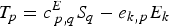
 is the elastic matrix (6 × 6) at constant electric field; e is the piezoelectric matrix (3 × 6) and
 is the dielectric matrix (3 × 3) at constant deformation. In practice, piezoelectric ceramics are poled in one direction. In this case, the model is reduced to only ten independent parameters: five elastic, three piezoelectric and two dielectric constants [2]. If losses are included, all parameters become complex constants [3]. Here complex material parameters are used for the constitutive equations; however, results are presented only for the real part of these parameters. The real part essentially determines the frequency of each resonant mode whereas the imaginary part determines the energy losses.
In recent years, a methodology to estimate the parameters in the piezoelectric model, based on the optimisation of a finite element simulation (FEM) to reproduce with high accuracy over a broad frequency band the complex impedance curves of a resonant piezoceramic disk was developed [4,5]. This approach not only opens new opportunities to use these elements but also to characterise slight variations between similar samples. This fact can be used to improve the fabrication process. For example; by studying how some changes in the fabrication process may affect a specific material parameter in the model, it might be possible to work towards improving certain properties in the final material. Other uses might include, for quality control in the fabrication process or to evaluate changes during the ceramic life cycle.
One of the objectives of this work was to find out if the results on the constitutive parameter model made using this methodology are good enough to detect these slight variations. The other objective was to determine the effect of aging over the parameters in the model.
After sintering, piezoelectric ceramics present spontaneous polarisation in the crystal structure when the temperature is below the Curie temperature. Inside the ceramic, ferroelectric domains grow to minimise the strains and charges created by the crystal distortion without generation of a macroscopic polarisation due to the random crystal orientation of the grains and charge compensation. This situation can be modified by heating and simultaneously applying an intense electric field. Due to the ferroelectricity, the electric dipoles within the domains align following the electric field and generate macroscopic polarisation. In this case the material presents macroscopic piezoelectric behaviour. Under the driving force of minimising the local electric or elastic energy, through different domain stabilisation mechanisms and irreversible microstructural changes, involving vacancies and defect dipoles, the material loses the macroscopic polarisation at a logarithmic rate with time, even remaining at rest. This effect is called aging [6,7].
Effects of aging are well known specially for commercial PZT ceramics. These are very stable and present small changes after several years. However, in the last years much effort has been made in the development of lead-free ceramics as suggested by environmental regulations [8]. Information on aging effects on these new materials is currently limited, but it is an important area of study, because it tells us about the stability of the material over time. Thus, we are looking for a technique to determine the aging effects in new materials. As a first approach, the technique was evaluated in a well-known material, the Pz27 from Ferroperm [9].
The present paper is an extended version of the results presented in the PIEZO2017, which took place in Cercedilla, Madrid. A set of Pz27 ceramic disks, thickness poled, was evaluated after 5 years without use, this way ageing effects are only due to spontaneous depolarisation. As the changes were very low, only one aspect ratio was used in this study, in order to reduce the variability of the results. The material parameters of a set of ten equal samples with thickness = 2 mm and diameter = 10 mm were estimated using the FEM optimisation approach.
FEM optimisation to determine the piezoelectric model
The use of FEM simulations allows the implementation of an iterative technique to obtain the parameters in the Equations (1a) and (1b). Usually we take the electrical impedance as the experimental data to be adjusted. Essentially, starting from a seed with a set of initial values for all parameters, the FEM obtains the simulated complex impedance and an error between results is computed. Depending on this error, the material parameters in the model are changed and the results are calculated again. The process is repeated iteratively until a desired level of error is achieved or until a preset number of simulations is reached. It is not the objective here to describe in further detail the algorithms used in the optimisation, which are described elsewhere [10]; only the relevant information for this particular work is given. The optimisation is made over all parameters [c11, c12, c13, c44, c33, e31, e33, e15, ε11, ε33], considering complex numbers to include losses. However results are given only for the real part, which essentially determines the frequency of each resonance.
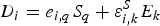
In this work, references to errors equate to the difference between modulus of impedance curves, thus, errors are defined as
One important fact is to assure the convergence of the FEM simulations. Here we are trying to detect slight variations among impedance curves, for this, the convergence error must be less than the difference between original impedance curves and the aged ones. All numerical simulations must use a finite size element to make the model. In FEM simulations the size of the element determinates the accuracy in the approximation of the results. Ideally we must use an infinitesimal element to reproduce all characteristics; however the simulation time grows with the square of the number of elements in this case. Then we must make a trade-off decision and fix a finite size for the elements. In this case, Equation (2) is evaluated using two numerical curves, one with a high number of elements, as a reference, and the other using the selected number of elements. The difference between the reference curve and other simulation using a smaller number of elements is called convergence error. The objective is to determine the size of the element with a convergence error less than the differences due to aging. To assure that we use a mesh size of 66 μm in the FEM simulations of the rotationally symmetric disk, corresponding to 30 elements in the thickness and 76 in the radial direction. Finite elements are implemented using our own code; the elements are square with four nodes and uses complex numbers for all parameters in the model. The geometry is bi-dimensional and is assumed axisymmetric; all computations are made in the frequency domain [5].
Experimental data
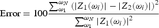
In order to evaluate the difference in the material parameters due to aging, a set of ten samples from the same fabrication process were used. For each sample the modulus and phase of the electrical impedance was measured using an HP4194A impedance analyser. To reduce the noise in the acquisition the average mode is used with 64 sweeps. Also each sweep is made using the medium integration time. Before making a measurement, the impedance of the wires and the sample holder were compensated. The same sample holder was used for both measurements, original and aged, this holder supports the sample using a very low force only at the centre point by using two needles. A 1000-point linear sweep over two frequency decades in the range [13 kHz to 1.3 MHz] was used. In this case, the frequency resolution was around 1.3 kHz. To evaluate if the resolution is good enough to reproduce the impedance curve we must take in to account the method to evaluate the function error, Equation (2). In this case the error is a sum over the complete frequency range, and the differences in a specific point do not have a great weight in the sum. Of course, to assure that all resonances are well sampled, we must have several points around each resonant frequency. As we can see in Figure 1, for this soft piezoelectric ceramic this requirement is fulfilled.
Results of the optimisation: modulus and phase of the electric impedance for a thickness = 2 mm, diameter = 10 mm Pz27 piezoelectric ceramic.
Measurements were performed on ten samples named S1 to S10. Two different measurements were taken for each sample: one in the original state and another after 5 years of aging. Ceramics had not been used for any other purpose before, and so all existing changes arise from spontaneous depolarisation (Figure 2).
Example of the changes in |Z| of a disk due to aging. As the differences are slight the effect is shown around the thickness mode.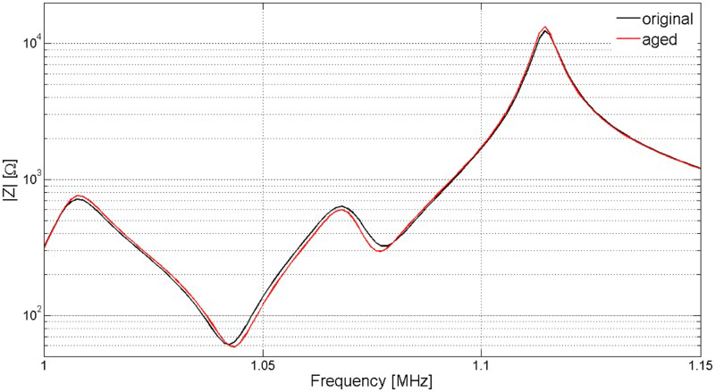
The changes in the resonance spectra between original and aged samples.

Table 1 shows differences on the order of 1% (mean 0.6, standard deviation 0.5). There is an appreciable variation between different samples. Therefore, similar variation in the evolution of parameters can be expected. The convergence error computed using the 66 µm grid is nearly 0.005%. This shows that using this mesh grid we have sufficient convergence to estimate the changes in the model.
Results
Mean and standard deviation std of the material parameters of the original samples (Ori), aged samples (Aged) and differences of the material parameters between original and aged samples (Δ).
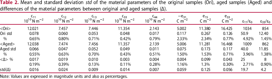
Note: Values are expressed in magnitude units and also as percentages.
The changes in each parameter is computed in absolute value and as a percentage calculated as follows:

The first row presents the parameters at the original state. The results are the mean value over the set of ten equal samples used in this work. The second row is the standard deviation of this set. The third row is the standard deviation expressed as a percentage of the parameter value. Next three rows are the same for the aged state. To compute the difference in the parameters, Equation (3) is used. In the last row, the standard deviation of the differences computed in the set is presented. For example, in the original state the set has a mean value of 12.021 for the stiffness c11, whereas in the aged state it has a mean value of 12.038. The standard deviation std of c11 values in the original state is 0.078, representing 0.65% of the mean value 12.021. At the bottom of the table, the difference between the mean of the original state values and the aged state of c11 has an absolute value of 0.017. This variation represents 0.19% of the original value, which are 12.021.
The standard deviations, obtained from the set of ten samples, represent the variation in the parameters due to dispersion in the fabrication process and not to the numerical estimation.
Figure 3 shows a detail of the differences between the experimental and numerical impedance curves in the region of the thickness mode for the original and an aged state. Both models fit very well the experimental data, with differences on the order of 1% or less for every fitting. However, these differences are the same in order as the differences between the original and aged samples.
Example of the differences between modelled and experimental |Z| in the original and in the aged sample. As the differences are slight the effect is shown around the thickness mode.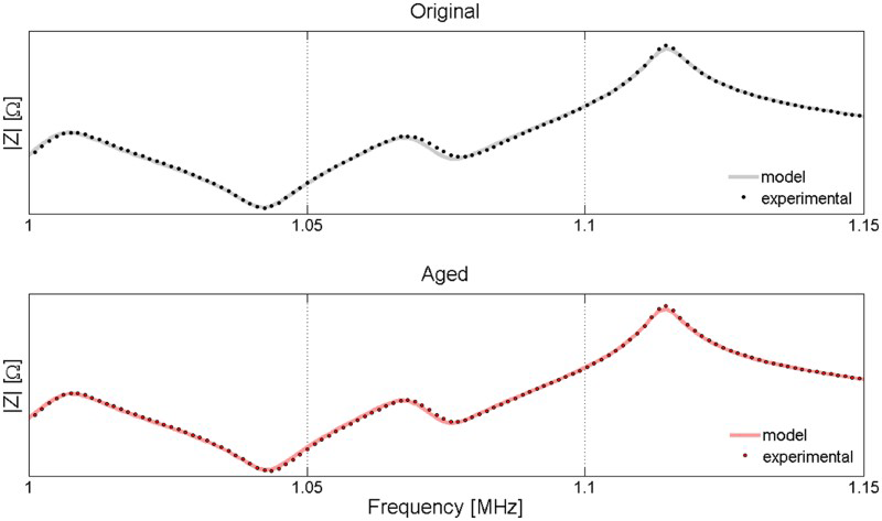
Conclusions
Errors between experimental and model computed using (2).

Thus, this methodology can detect tendencies in the parameters, although the variation detected was quite small to produce significant variations. The low variation between both states, original and aged, can be attributed to the large stability of PZT ceramics.
For this material, the parameters in the model have a low dispersion when computed for the ten ceramics set; the dispersion between the values of one individual parameter (Table 2) is on the order of 1%. Three parameters have higher standard deviations: e31, e15 and ε11. These parameters have the lowest sensitivity (i.e. the effect on the error between experimental data and FEM simulations is influenced only in a minor way by changes in this parameter) in the model [10]. Hence, the large variations for these parameters can be assigned to the numerical methodology used to determinate its value and not to the fabrication process.
The higher source for error between experimental and numerical data is in the model used for the FEM calculation. The model assumes a perfect disk and a homogeneous material without spatial variations in the properties. However, real ceramics are not homogeneous and may have parallelism and centralisation errors. The main source of error, therefore, is not on the optimisation technique, but in the hypothesis in the formulation of the finite element method. Note that, due to computational cost, the model must be axisymmetric.
As a summary of the changes detected for this specific set of ceramics we can divide the parameters in two different categories: if the mean value of the change for a specific parameter is equal or greater than the standard deviation, we conclude that a variation is detected, otherwise one cannot draw conclusions about this parameter. Using these criteria, elastic stiffness c11 and c13 increases, whereas the dielectric constants approach each other, that is, ε33 decreases its value whereas ε11 increases.
Footnotes
Acknowledgements
The authors thank ‘JECS Trust grant for attendance to the Winter School on Advanced Characterization of Piezoceramics, Cercedilla, Madrid (Spain). 19–22 February 2017’.
Disclosure statement
No potential conflict of interest was reported by the authors.