
Abstract
Prior studies have separately suggested the importance of physical distance or social distance effects for the creation of neighborhood ties. This project adopts a case study approach and simultaneously tests for propinquity and homophily effects on neighborhood ties by employing a full–network sample from a recently developed New Urbanist neighborhood within a mid–sized southern city. the authors find that physical distance reduces the likelihood of weak or strong ties forming, suggesting the importance of accounting for propinquity when estimating social tie formation. the authors simultaneously find that social distance along wealth reduces the likelihood of weak ties forming. Social distance on life course markers—age, marital status, and the presence of children—reduces the formation of weak ties. Consistent with the systemic model, each additional month of shared residence in the neighborhood increases both weak and strong ties. An important innovation is this study's ability to directly compare the effects of physical distance and social distance, placing them into equivalent units: a 10 percent increase in home value difference is equivalent to a 5.6 percent increase in physical distance.
Social Space and Physical Space: Homophily, Propinquity, and the Formation of Neighborhood Ties
A central question of sociology concerns the relationship between physical space and social space. That is, to what extent are social ties predicated upon physical proximity? the general question holds major implications for numerous areas of social research, including segregation in housing and education (Krysan and Farley, 2002), political deliberation (Putnam, 2000; Perrin, 2006), environmental preservation, health behavior (Gordon–Larsen et al., 2006), and more. Recent technological developments may have changed individuals’ ability to form and maintain social ties across greater physical distances (Fischer, 1992; Wellman and Hampton, 2001), while simultaneously reducing the importance of face–to–face interaction (Putnam, 2000).
Urban theorists have long been interested in the determinants of social ties between neighbors. This interest in tie formation is unsurprising given theories positing that ties lead to neighborhood satisfaction (Sampson, 1991) and neighborhood cohesion (Kasarda and Janowitz, 1974; Sampson, 1988; Hipp and Perrin, 2006), or that social ties heighten the ability of neighborhoods to band together collectively to reduce crime and disorder (Freudenburg, 1986; Sampson, Raudenbush, and Earls, 1997) and even to challenge political decisions that might otherwise threaten the community itself (Tilly, 1974; Guest, 2000). Indeed, a key focus of the New Urbanist movement is an attempt to increase the number of social ties between residents by implementing various design features (Kleit, 2005; Talen, 2006). One approach adopted by a line of research assesses the characteristics of household members with a greater number of ties in the neighborhood. Besides looking at household characteristics, this line of research also suggests that the context of the neighborhood—specifically, certain types of social distance within the neighborhood—will reduce the number of ties that exist. the term “social distance” refers to the salience of certain social characteristics that form both an awareness of similarity with others based on the characteristic and an awareness of difference with others not sharing the characteristic; this refers to such dimensions of social life as race/ethnicity, socioeconomic status, or religion (Poole, 1927; McPherson and Ranger–Moore, 1991). a second approach focuses on which ties exist in the neighborhood, rather than the total number. in this second approach, two key characteristics have been postulated: (1) a physical distance (or propinquity) effect in which households tend to create ties with other households closest to them, with the probability of a tie decaying with distance from the household (Zipf, 1949), and (2) a social distance effect in which households form ties with other households most similar to them along various demographic characteristics. While studies have looked at each of these two characteristics in isolation, almost no studies have considered them simultaneously.
When asking to whom individuals are tied, a key characteristic to consider is simply how physically close the neighbors are. Zipf (1949) suggested that individuals attempt to minimize effort by interacting with those physically closest to them. This notion of a propinquity effect—that individuals will tend to associate most with those closest to them in physical space—was observed in two classic studies in the early 1950s that controlled for social distance through their study design by focusing on a homogeneous population (Caplow and Forman, 1950; Festinger, Schachter, and Back, 1950). 1 While these studies provided keen insights regarding propinquity effects, their approach of controlling for social distance effects by studying a homogeneous population leaves unexplored the possibility that social distance effects will dominate physical distance effects as heterogeneity increases.
The notion of “social distance” is a fundamental concept in sociology (Poole, 1927) and is based on difference in statuses among individuals. Sometimes referred to as “Blau–space” (McPherson and Ranger–Moore, 1991), it is associated with such characteristics as race/ethnicity, economic resources, gender, life course stage, and social background. a broad literature has studied the importance of social distance for the formation of various types of social ties: neighborhood ties, workplace ties, organizational ties, or even multiple dimensions of ties simultaneously, generally finding considerable preference homophily effects along various social dimensions (Lazersfeld and Merton, 1954; Feld, 1982; Blau, Ruan, and Ardelt, 1991). However, since these studies nearly always necessarily ignore possible propinquity effects, it is uncertain whether such findings indeed reveal a homophily preference or simply the constraints of the local context. McPherson and Smith–Lovin (1987) termed these constraints of the local neighborhood “structural homophily,” since they reflect structural characteristics formed by exogenous forces. Researchers studying classroom network relations are aware of this possible contextual problem, and recent work has shown the importance of taking into account the socio/demographic context in which tie formation takes place (Quillian and Campbell, 2003; Mouw and Entwisle, 2006). Thus, despite the theoretical expectation that social distance will impact the formation of neighborhood ties, we have little evidence of which, if any, demographic characteristics are important.
Determining the origins of social ties is both conceptually and methodologically challenging. Conceptually, social ties may form and dissolve as a result of exogenous realities (e.g., physical and class mobility, life course effects) or as a result of other social ties. Methodologically, discerning the effects of physical space from the social preferences emerging from social space requires a full–network survey with independent measures of physical and social space, a particularly difficult task when studying the residents of an entire city. We provide such an examination here by employing a case study approach for one specific neighborhood in a city. This allows us to zero in on the dual effects of preference homophily and propinquity for one specific type of social tie—neighborhood ties.
We address the homophily versus propinquity question by studying all residents in a particular neighborhood of a mid–sized community in the south. We employ a full network design in which residents are given a roster of all other residents in the neighborhood and asked with whom they interact in various manners. This approach allows us to simultaneously take into account physical distance effects (since we know the exact location of the respondents’ housing units) and social distance effects (since we know the demographic characteristics of all the respondents to the survey). We focus on a New Urbanist community, in part because one important principle behind this approach is that by locating mixed housing in close proximity, social interactions between residents of different economic classes will be fostered (Talen, 2006). We are able to assess to what extent this principle is actually achieved in this particular neighborhood. While another study focused on social ties in a New Urbanist neighborhood as measured by ego–networks (Kleit, 2005), our approach using a full network design can more appropriately account for propinquity effects.
In what follows, we begin by describing why various characteristics of social distance should have effects on the formation of neighborhood ties. We then describe our sample and the methodology employed. Following that, we describe our results focusing on the determinants of tie formation between residents in this neighborhood. After presenting the results in which social distance effects are translated into physical distance units, we summarize our results and conclude with implications.
Physical and Social Distance and Tie Formation
While the notion that physical distance negatively affects interaction has a long history, we explore here the importance of a more general conceptualization of distance. Thus, we consider both physical and social distance and suggest that both can be attributed to an underlying principle. Early on, Zipf (1949) suggested that individuals follow a principle of least effort expended, and that this can explain propinquity effects. Mayhew and Levinger (1977, p. 93) built on this concept in positing a macro effect of physical distance on the form of ties observed in a metropolitan area and noted the Law of Distance–Interaction: the “likelihood of interaction or contact of any kind between two social elements is a multiplicatively decreasing function of the distance between them, or of the costs of overcoming that distance.” Thus, if individuals attempt to minimize effort, they will form ties with other individuals who are closest to them in physical space, ceteris paribus. Mayhew et al. (1995) extended this energy distribution principle from propinquity to the notion of social distance. Thus, they highlighted that the tendency to prefer communication with others who speak the same language can be considered a special case of the energy distribution principle. and it is straightforward to extend this notion of sharing the same language to other characteristics that create shared cultural cues. More recent work by Butts (Forthcoming) has formalized this general concept of distance, suggesting that physical and social distances are simply special cases of this more general principle. However, empirical work has failed to simultaneously address the effects of physical and social distance on neighborhood tie formation.
The notion of “social distance” can be observed along several different social categories. a long line of literature has suggested that economic inequality creates classes that foster social distance (Marx, 1978). Thus, while there is minimal social distance between any two members within a particular class, there is considerable social distance between any two members of different classes. in the twentieth century, the importance of racial/ethnic differences has come to dominate and define measures of social distance and is posited to cause such outcomes as racism, group conflict, and segregation (Green, Strolovitch, and Wong, 1998; Massey and Denton, 1987; Sampson, 1984; South and Deane, 1993; Tajfel and Turner, 1986). Nonetheless, social distance can also be created by various other characteristics such as cultural values, social background, or stage of the life course, and Blau (1977; 1987) built on the work of Simmel (1955) to focus on the degree of overlap between individuals in these various categories or “cross–cutting circles”. This perspective focuses on the distance between individuals in social space, rather than physical space, suggesting that it will reduce social interaction. But why might social distance reduce social interaction among individuals? We next consider three possible mechanisms.
Mechanisms of Social Distance
Past theory and research suggests three reasons why social distance might be important for affecting interaction between residents: (1) social distance can decrease the similarity in attitudes between two individuals; (2) social distance can decrease the chances of creating a shared group identity; and (3) social distance, as exemplified by social statuses, creates role differences. We consider each of these next.
First, Bourdieu (1984, pp. 476–477) argued that the social position of individuals affects their attitudes and cultural preferences. An individual's social origin shapes their views and attitudes throughout life, what Bourdieu referred to as “habitus”, creating social distance from those with different social origins. Thus, the awareness of others’ different social background will discourage interaction based on the expectation of a lack of common social ground.
Second, a long line of social psychology literature suggests that individuals with even superficial similarities can come to categorize themselves and others as members of the same group (Friedkin, 1999; Hogg, 1992; Simon, Hastedt, and Aufderheide, 1997; Turner, 1987). Once an individual self–categorizes him/herself into a particular group, self–categorization theory (Tajfel and Turner, 1986) posits that: (1) individuals will expect to agree with those who are functionally identical; (2) failing to agree with similar others will increase subjective uncertainty; and (3) the views of similar others will be influential as they provide feedback on the social validity of one's own views (Fleming and Petty, 2000). This suggests that groups fostered by similarity on social categories are important for providing self–validation and order to the world (Lau, 1989). the repeated interaction of group members will foster group identity, leading to even more interaction among those closer socially.
Finally, in social status theory (Merton, 1968) individuals inhabit social positions (or “social statuses”) that are accompanied by appropriate social roles. There are then various role expectations associated with each position, and we might expect these to lead to differences in the actions, cultural cues, and attitudes of an individual in one position compared with someone in another position. in network terminology, such individuals can be described as occupying structurally equivalent positions. Many statuses are categorical, bringing about social distance. for instance, consider marital status: membership in the social position of “married” precludes simultaneous membership in the social position of “single.” Thus, social status theory argues that the roles associated with these positions lead to different lifestyles that will sometimes minimize interaction between those in different statuses.
Determinants of Social Distance
Given these mechanisms of social distance, the question then is what social characteristics might be particularly important for fostering distance that reduces social interaction. Theoretical models have suggested five key determinants of social distance: (1) economic class; (2) life course position; (3) cultural values and attitudes; (4) gender; and (5) racial/ethnic differences. We are unable to test for the effects of racial/ethnic differences here as, common to many neighborhoods in the U.S., our study neighborhood is nearly perfectly homogeneous (ours is almost completely white). Nonetheless, we are able to test for the effect of these other dimensions while holding race/ethnicity constant. We consider each of these determinants of social distance next.
Arguably the most fundamental sociological determinant of social distance is economic class. While Marx (1978) articulated this as a dichotomous measure of differing classes, Weber (1968) expanded this to include a broader conception of social class that functioned more like a continuous measure. Weber's conceptualization included one's education level and the prestige of one's occupation. Recent works in this tradition have viewed economic inequality as social distance between individuals that leads to strain and hostility (Morenoff, Sampson, and Raudenbush, 2001; Hipp, 2007). Again, a key New Urbanist principle is the notion of bringing together in close proximity those of different socioeconomic backgrounds in the hope that it will foster social interaction across income levels (Talen, 2006). to the extent that income differences lead to reduced interaction between residents, this suggests an important implication for low–income housing policies.
The life course perspective has advanced the view that social positions fundamental to most societies—age, marital status, and presence of children—are important for creating social distance and reducing interaction (Michelson, 1976; La Gory and Pipkin, 1981; Elder, 1985, 1998). Age is particularly important for creating social distance, as birth cohorts experience different life events that create social distance in attitudes and viewpoints (Elder, 1999). Additionally, children are grouped in classrooms based on age, while “homogamy on age in marriage is so taken for granted that it is seldom even studied” in research of the U.S. (McPherson, Smith–Lovin, and Cook, 2001). Studies of factory workers (Feld, 1982) and persons aged 60 and over (Ward, LaGory, and Sherman, 1985) also found age homophily effects. Besides age, marital status and the presence of children are important determinants of social distance. Marital status leads to lifestyle differences from those who are single (Fischer, 1982), while the presence of children creates a host of role expectations that result in considerable lifestyle differences from those without children (Stueve and Gerson, 1977; Fischer, 1982). Indeed, recent work using ego networks has found that both marital status and age have important effects on tie formation (Kalmijn and Vermunt, 2007).
A third possible determinant of social distance comes from cultural, or attitudinal, differences. Thus, rather than structural characteristics giving rise to social distance, belief systems and values may give rise to social distance (Huckfeldt, 2004). for instance, a voluminous literature has focused on the possible importance of religion for fostering social distance between individuals in such things as attitudes and value systems, and even in dietary practices (Durkheim, 1915; Fischer, 1982; Bellah et al. 1985). Likewise, considerable scholarship suggests that political differences spring from differing value systems (Mouw and Sobel, 2003): if this is the case, we might expect this to reduce the formation of close ties and possibly even reduce the formation of weak ties within neighborhoods.
A fourth possible determinant of social distance is gender. Feminist scholarship has pointed out differences in the structural characteristics faced by men and women leading to differences in life chances (Beggs, 1995; Kalleberg, Reskin, and Hudson, 2000; Cohen and Huffman, 2003). If an awareness of these structural differences is fostered, one would hypothesize that this could lead to social distance that would inhibit the formation of neighborhood ties. on the other hand, the dyadic, balanced nature of most households on gender suggests the possibility that such social distance would not be fostered and thus not have an effect on the formation of neighborhood ties. We test these countervailing predictions here.
Despite the theoretical expectation that social distance will matter for the emergence of social ties within neighborhoods, there is actually minimal empirical evidence. While studies have frequently tested for the individual– and neighborhood–level predictors of the presence of more reported neighborhood ties by residents, testing for social distance effects in such studies would require cross–level interactions. That is, simply testing whether the presence of more households with children affects the number of neighborhood ties (Campbell and Lee, 1992; Logan and Spitze, 1994) implicitly tests whether all households in such neighborhoods report more ties. Testing for social distance effects requires testing whether households with children report more social ties in neighborhoods with a higher proportion of children—that is, a cross–level interaction between these two constructs. While studies testing for the effects of racial/ethnic heterogeneity on the number of neighborhood ties reported by residents come closer to testing for social distance effects, they still suffer from the ecological inference problem (Robinson, 1950) since they are not directly testing whether it is the individuals who are in the racial/ethnic minority who have the fewest social ties.
Finally, a limitation of most previous studies of social distance effects is their failure to take into account possible physical distance effects. If people simply prefer to interact with those physically closest to them—and neighboring households are socially similar—studies would incorrectly conclude that social distance effects are present. Butts and Carley (1999, p. 7) suggest that “fitting a gravity model on data with physical and social special dimensions will yield social distances in physical equivalents; thus, in principle one could ascertain the ‘extra distance’ in km between persons of differing race or gender.” to our knowledge, our study is the first to empirically attempt to measure these social distances in this manner, and we are able to provide estimates of these social distances “in physical equivalents.”
Data and Methods
Our data come from a survey conducted in a relatively new neighborhood of about 150 housing units in the southern United States. Thus, our “neighborhood” is about 20 percent as large as the typical block group—a unit of analysis that, some have suggested, may capture most local interactions (Grannis, 1998). the first houses were built in 2001 in this “New Urbanist” development within a city of approximately 50,000 residents, meaning it includes several different kinds of housing units, ranging from rental apartments and “affordable” townhomes to luxurious custom homes costing as much as $2 million. in addition, a “downtown” area includes a grocery store, restaurants, shops, and services. There are medical services, a retirement community, a health club, and an outdoor pool in the complex. the residents are mostly middle– and upper–middle income white homeowners in this neighborhood just a couple of miles from the downtown of the city in which it resides. This neighborhood is adjacent to other city neighborhoods and thus is not geographically isolated.
We obtained a list of all units in the neighborhood from the development's homeowners’ association. We conducted the mail survey in the Fall of 2003, employing many of the “total design” techniques of Dillman (1978): we mailed an introductory letter and the survey instrument to all adult respondents in the household; we then followed up with a postcard reminder one month later; and then two months later we sent a letter reminder to those who failed to complete the survey and mailed a new survey instrument to those who no longer had the one from the initial contact. We utilized techniques such as using stamps on enclosed self–addressed return envelopes rather than a postage meter or business reply mail. the result of these various techniques was a final response rate in which at least one member of 42 percent of the households returned completed surveys. 2 When more than one adult of the household returned a survey, we included both in our analyses (we describe below how we take nonindependence into account in the analyses). Our analyses are performed on dyads constructed from the 87 respondents returning surveys and the residents they named (since we have some information on nonrespondents, such as physical location and value of home). Given that we attempted to contact all respondents, this is actually a census of these residents.
Outcome Measures
Our key outcome measures are zero/one indicators of whether the dyad is linked in some manner. We provided survey respondents a list of all residents in the neighborhood and asked them which neighbors they: (1) talk to; (2) visit in their homes; (3) communicate with by email; (4) communicate with by phone; and (5) feel close to. 3 We labeled as weak ties those dyads in which the respondent reported any of the first four types of interaction with the other member of the dyad but did not report feeling close to them. If the respondent reported feeling “close to” the other member of the dyad, we counted this as a strong tie. We feel confident using this measure of “closeness” as a measure of tie strength since Marsden and Campbell (1984) found in a multiple indicators study that closeness is the best indicator of tie strength. in additional models, we considered the outcome of the number of shared ties of any type as a mediating variable.
Exogenous Measures
Our key predictor variables are dyad measures capturing the degree of difference between the two households/respondents constituting the members of the dyad. 4 to measure the physical distance of housing units from one another, we linked information on the latitude and longitude for each housing unit in our sample from the tax roles in the state where our sample was taken. We were then able to compute the direct distance between each set of households in the sample. Since there is reason to expect that distance exhibits a decay effect—as suggested by Zipf (1949)—we natural log transformed this measure. 5
We also included several measures of social distance. Note that we are assuming that these various social dimensions enter into the model additively: we performed exploratory tests for interactive effects between these dimensions and found none. to measure the effects of socioeconomic status on social interaction, we linked information on housing values from the tax roles in the state where our sample was taken to the survey respondents. Using housing values as a measure of socioeconomic status is more desirable than using such SES measures as income or education because (1) the value of the home is often more readily apparent than is the income or education level of the household members (making more readily apparent the social distance between the dyad members), (2) the value of the home is one of the strongest measures of wealth in the contemporary U.S., and (3) the seven–point Likert scale we used to measure income is a rather crude measure of income, in contrast to the more fine–grained measure possible when using housing value. We natural log transformed this measure since the effects of distance on home value likely have a diminishing effect and to minimize the presence of outliers.
We also measured difference between households along three key life course characteristics: age, marital status (classified as married or not), and the presence of children in the home less than 18 years of age. for each dyad of respondents, we computed the difference between the two households on each of these characteristics. Thus, if both households were married, or if both households were single, they would get a value of zero for the measure of difference in marital status. But if one household were married while the other was single, the dyad would get a value of one for the measure of difference in marital status. Thus, higher values for these measures capture greater social distance.
To capture possible cultural differences, we calculated social distance on three measures. Since southern culture may evoke unique characteristics, we took into account whether or not the respondents were born in the south. to account for possible differences in political persuasion, each respondent assessed their degree of liberalness on a seven–point Likert scale. 6 Our dyad measure thus calculated the absolute value of the difference between the two respondents on their assessments of this measure. to account for religious differences, each respondent assessed how important religion is to their life in a five–point Likert scale. 7 Again, our dyad measure calculated the absolute value of the difference between the two respondents on their reports to this measure.
While our study is of a relatively new neighborhood, there may nonetheless be important effects for the length of residence in the neighborhood. We took this into account in two manners. First, the systemic model (Kasarda and Janowitz, 1974) and social disorganization model (Sampson and Groves, 1989) both suggest that residents who have lived longer in the neighborhood will know more neighbors, and empirical evidence suggests that in neighborhoods with more residential stability residents will report a greater number of social ties (Connerly and Marans, 1985; Sampson, 1988; Sampson, 1991; Logan and Spitze, 1994; Warner and Rountree, 1997; Ross, Reynolds, and Geis, 2000). We accounted for this by including a measure of the shared length of residence for the respondents—that is, the minimum length of residence in months for the two members of the dyad. Second, we tested whether dyads whose members have lived in the neighborhood for similar periods of time—and thus share membership in a neighborhood cohort—are more likely to form ties. We constructed a measure of the difference in months in length of residence for the two members of the dyad. We also accounted for possible gender effects with a measure of the difference of the dyad based on gender.
Finally, since we are using dyadic data, we included network measures to account for the nonindependence of the dyads. Following Moody (2001) and Mouw and Entwisle (2006), we included four network measures: (1) the number of ties nominated; (2) the number of ties received; (3) whether the alter nominated the respondent (reciprocity); and (4) the number of shared ties (mutuality). We point out that there is some uncertainty whether it is appropriate to include such network measures in the model, or whether their inclusion constitutes over–specification (Quillian and Campbell, 2003). Mouw and Entwisle (2006) pointed out that controlling for these network measures provides an estimate of the direct causal effect independent of these measures, but that they can also be considered as mediating factors. We do so briefly down below. the summary statistics for the variables used in the analyses are shown in table 1.
Summary Statistics for Variables Used in Analyses of Survey of Respondents Conducted in a Relatively New “New Urbanist” Neighborhood of about 150 Housing Units in the Southern United States
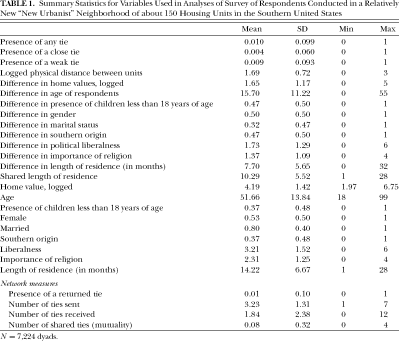
N= 7,224 dyads.
Methodology
Since our main outcome measures were dichotomous, we assumed a logit distribution. to account for the nonindependence of observations (since each respondent is reporting on the existence or lack of a tie with each of the other residents in the neighborhood), we employed an exponential random graph (p*) model, in which we included the four network measures described above to account for this dependence (Anderson, Wasserman, and Crouch, 1999; Pattison and Wasserman, 1999; Pattison and Robins, 2002). to account for missing data, we used multiple imputation. Given that the level of missing data was less than 5 percent for individual variables, imputing five data sets provided a satisfactory degree of information for our sample (Schafer, 1997). Multiple imputation allows utilizing the information from all cases and requires the less stringent assumption of missing at random rather than list–wise deletion's assumption of missing completely at random (for a complete discussion of the distinction between types of missing data, see Rubin, 1976; Rubin, 1987). All models were estimated in Stata 8.0. for the model with the count of number of shared ties as the outcome, we employed a negative binomial regression model.
Results
Determinants of the Presence of a Weak Tie
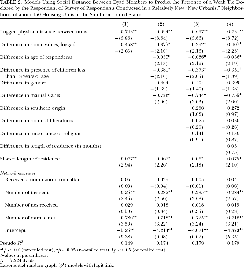
We begin by viewing the predictors of the presence of a weak tie between dyad members. Focusing first on the two key characteristics of propinquity and socio/economic differences, we see in model 1 of table 2 the expected inhibiting effects for both of these measures. Greater logged physical distance between the two members of the dyad reduces the likelihood of a weak tie, and greater difference in the logged value of the homes of the members of the dyad also reduces this likelihood. Both of these effects are quite substantial and quite robust: they remain significant and only diminish somewhat in the following models including the other determinants of social distance. for instance, when we include all of our social distance measures in model 4, a one–unit increase in logged physical distance between households results in a 52 percent reduction in the likelihood of the presence of a weak tie. 8 Also, a one–unit increase in the difference of logged home values in this same model results in a 33 percent reduction in the likelihood of a weak tie. If we assume that a one–standard deviation change is equally plausible for each of these predictors, we would conclude that they have almost identical effects on the likelihood of a weak tie being present (the odds are reduced about 40 percent). Thus, we see evidence that wealth differences reduce casual interaction between residents, even controlling for the physical distance between their units and our other measures of social distance.
Models Using Social Distance Between Dyad Members to Predict the Presence of a Weak Tie Declared by the Respondent of Survey of Respondents Conducted in a Relatively New “New Urbanist” Neighborhood of about 150 Housing Units in the Southern United States
p < 0.01(two–tailed test),
p < 0.05 (two–tailed test),
p < 0.05 (one–tailed test).
t–values in parentheses.
N= 7,224 dyads.
Exponential random graph (p*) models with logit link.
In model 2 we add the effects of four life course measures. All four measures show the expected negative effect on the presence of a weak tie, although difference in gender does not achieve statistical significance in this sample for a one–tail test at p < 0.05. the effects for age differences are robust, and remain in the subsequent models including additional dimensions of social distance. for instance, in model 4, with all of our social distance measures included, a one–standard deviation increase in the difference in age between the members of the dyad (about 11 years) results in a 33 percent reduction in the likelihood of a weak tie. 9 a similarly strong effect is found for dyads that differ on the presence of children under the age of 18: differing on this characteristic reduces the likelihood of a weak tie about 30 percent in model 4. Also, difference along marital status has an even stronger effect, as dyads differing in marital status are about 53 percent less likely to forge a weak tie compared with dyads similar on this characteristic. in addition, since these effects are additive, a dyad in which one member is married with children and the other is single with no children is 67 percent less likely to form a weak tie than a dyad similar on both of these measures (exp(–0.351 – 0.755) = 0.331).
In models 3 and 4 including our measures of social distance along cultural characteristics and difference in length of residence in the neighborhood, we find no significant effects. Thus, there is no evidence in this sample that difference in southern origin or difference in political liberalness reduces the likelihood of a weak tie among the dyad members. Also, while difference in the importance of religion shows a modest negative effect on the likelihood of a weak tie, it does not come close to statistical significance at p < 0.05. Finally, there is no evidence in model 4 that difference in length of residence reduces the probability of a weak tie between dyad members.
Determinants of the Presence of a Strong (Close) Tie
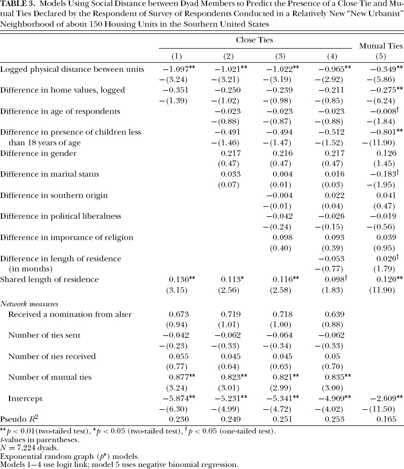
We next test whether the determinants of a tie labeled as “close” differ from those of the weaker ties just tested. Paralleling our strategy for testing the effects of weak ties, we begin with a model testing the effects of propinquity and differing home values in model 1 of table 3. the effect of physical propinquity on the presence of close ties in this model is similar to, and even stronger than, its effect on weak ties. a one–unit increase in the logged physical distance between the members of a dyad reduces the likelihood of a close tie about 62 percent in model 4 including all of our social distance measures. These strong propinquity effects highlight the importance of taking into account the physical distance between residents: studies viewing the demographic composition a resident's neighborhood ties while failing to take into account the characteristics of nearby households thus risk obtaining biased results.
Models Using Social Distance between Dyad Members to Predict the Presence of a Close Tie and Mutual Ties Declared by the Respondent of Survey of Respondents Conducted in a Relatively New “New Urbanist” Neighborhood of about 150 Housing Units in the Southern United States
p < 0.01(two–tailed test),
p < 0.05 (two–tailed test),
p < 0.05 (one–tailed test).
t–values in parentheses.
N= 7,224 dyads.
Exponential random graph (p*) models.
Models 1−4 use logit link; model 5 uses negative binomial regression.
On the other hand, although we see no evidence that the other distance measures in this model have a direct effect on the likelihood of a close tie forming, there are some effects of the network measures. of the four network measures we include in these models, it is notable that the measure of shared ties (mutuality) has a strong positive effect on the formation of both weak and close ties. for instance, each additional mutual tie increases the odds of a weak tie forming by about 2.3 times, and approximately doubles the odds of a close tie forming. These are very strong effects and highlight the importance of such mutual ties. Mouw and Entwisle (2006) pointed out that network measures such as mutuality are endogenous measures in this process, which allows estimating the total effect of these distance measures on the likelihood of close or weak ties by estimating models without the network measures. the logic is that, whereas these distance measures give rise to network ties, some of these created ties will be mutual, which will then create additional ties. Thus, these mutual ties in part mediate the relationship between the distance measures and tie formation.
To test this possibility, we estimated a model predicting the number of shared ties for a dyad. the results are presented in model 5 of table 3, and highlight that social distance based on socioeconomic difference, age, marital status, and the presence of children all reduce the likelihood of mutual ties forming. as well, physical distance also reduces the formation of mutual ties. the effect of distance based on the presence of children is particularly strong and suggests that whereas we did not detect a significant direct effect of this measure on the formation of close ties, there is an indirect effect through this formation of mutual ties. in support of this, we estimated a model predicting the presence of a close tie that did not include the four network measures and found that distance based on children was about 25 percent larger and significant at p < 0.05 for a one–tail test (results not shown). This suggests that distance based on the presence of children largely reduces the likelihood of a close tie because it reduces the number of friends in common.
We also highlight the strong effects for the measure of shared length of residence on the formation of both weak and strong ties in these models. for instance, an increase of 5 ½ months in shared length of residence in the neighborhood (one–standard deviation) increases the likelihood of a strong tie by about 71 percent and a weak tie by about 50 percent. as well, this shared length of residence has a strong effect on the presence of shared ties: an additional 5½ months of shared length of residence essentially doubles the number of shared ties. Given that these shared ties then lead to more weak and close ties, we see substantial support for the systemic theory hypothesis that increasing shared length of residence in the neighborhood will increase the likelihood of neighborhood tie formation, at least among this sample of a relatively new neighborhood.
Placing Social Distance Effects into Physical Distance Metric
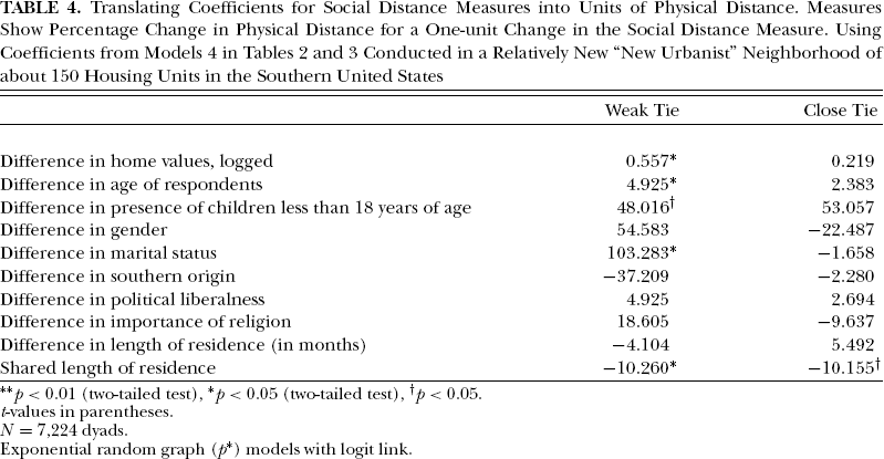
Finally, we translate the social distance measures from the above models into physical distance units to compare the magnitude of the effects. This follows the suggestion of Butts and Carley (1999, p. 7) that such a model can “yield social distances in physical equivalents.” While we caution that these estimates come from this study of a single community, we suggest that this exercise is nonetheless illustrative of what can be accomplished with this technique. to accomplish this, we used the estimates from model 4 in table 2, and model 4 in table 3 to (1) calculate the effect of a 1 percent change in physical distance (0.01 log units in physical distance ×β1, where β1 is the estimated coefficient for physical distance) and (2) divide the coefficient for a particular social distance construct (β2) by the value in (1). This translates a one–unit change in the social distance measure into the percentage change in physical distance (since this measure was log transformed), and the results are presented in table 4. for instance, a 10 percent increase in the difference in home values between dyad members is equivalent to a 5.6 percent increase in the physical distance between them in the model for weak ties. Each additional year difference in age between the dyad members is equivalent to moving 4.9 percent farther away in the model for a weak tie. There are strong effects for the presence of children: differing on the presence of children is equivalent to moving 48 percent further away in the weak ties model, and equivalent to moving 53 percent further away in the close ties model. Differing on marital status is approximately equivalent to doubling the physical distance between residents. Finally, each month shared residence in the neighborhood shows strong effects, as it is equivalent to moving 10 percent further away in both the weak ties and close ties models. 10
Translating Coefficients for Social Distance Measures into Units of Physical Distance. Measures Show Percentage Change in Physical Distance for a One–unit Change in the Social Distance Measure. Using Coefficients from Models 4 in Tables 2 and 3 Conducted in a Relatively New “New Urbanist” Neighborhood of about 150 Housing Units in the Southern United States
** p < 0.01 (two–tailed test),
p < 0.05 (two–tailed test),
p < 0.05.
t–values in parentheses.
N= 7,224 dyads.
Exponential random graph (p*) models with logit link.
Conclusion
Our sample of a New Urbanist neighborhood in a mid–sized southern city has provided key insights into the effects of social and physical distance for the formation of one particular type of social tie: neighborhood ties. While the possibility of propinquity effects on tie formation is well known, and two previous studies showed these effects for the formation of neighborhood ties (Caplow and Forman, 1950; Festinger, Schachter, and Back, 1950), studies rarely take these possible effects into account. By accounting for the demographic composition of the neighborhood, we were able to test the degree to which neighborhood ties form due to choice as opposed to simple constraint due to neighborhood composition. By taking into account propinquity effects, we were able to assess whether social distance matters above and beyond the effect of propinquity. Thus, by simultaneously estimating the effects of physical and social distance, our model yields what Butts and Carley (2000, p. 7) refer to as “social distances in physical equivalents.” We are aware of no other study that has tested this using neighbor networks.
Simultaneously testing the effects of physical and social distance has highlighted the importance of both. the strong effects of physical distance for various forms of ties provide a cautionary note for studies testing homophily effects, without accounting for the context in which those ties form. the evidence here is clearly consistent with the notion that residents choose those closest to them when choosing with whom to interact. While this physical distance is important for the formation of weak ties between neighbors, it has an even stronger effect on the formation of close ties between residents. Thus, taking into account the characteristics of the neighbors physically closest to a resident is important for determining homophily preferences.
Nonetheless, we found that certain dimensions of social distance matter even when accounting for such propinquity effects. Most notably, we found that difference in home values of the dyad members reduces the formation of weak ties. Note that although similar valued homes tend to be located physically close to each other, our study took this into account by controlling for the physical distance between households. This socioeconomic difference also has an indirect effect on tie formation by reducing the formation of mutual ties, which are important for fostering both strong and weak ties. These findings have important implications for the flow of information within a neighborhood and the building of cohesion that might foster the ability to band together in times of neighborhood stress (Sampson, Raudenbush, and Earls, 1997; Morenoff, Sampson, and Raudenbush, 2001). Whereas many analysts rightfully lament the wealth differences among neighborhoods that likely lead to differences in political interests engendering splintering of the polity (Tilly, 2003), our findings suggest that wealth differences affect the degree of social interaction between residents within relatively small neighborhoods as well. This has important implications for theoretical models such as the social disorganization theory positing that reduced interaction will increase neighborhood crime rates—based on our findings that income/wealth disparity in a neighborhood reduces weak ties between dyad members, future studies will want to test whether this leads to a macro structural effect in which neighborhoods with more inequality have fewer social ties overall. Past research in the social disorganization literature has generally failed to test the effect of neighborhood inequality on tie formation (for an exception, see Hipp, 2007).
This effect of wealth inequality may also imply important policy implications for the New Urbanist perspective, as it suggests a need for more active efforts to bridge the gap between residents of different economic backgrounds. While New Urbanist developments that place units of differing values nearby may help cohesion—as our findings regarding the importance of propinquity imply—our findings suggest that this will not be enough to bridge these economic differences that appear to inhibit the formation of social ties. to the extent that such ties are important for fostering community cohesion and collective action, policymakers would need to directly address this through efforts aimed specifically at bringing these different economic groups into direct contact with one another.
And while studies testing the effect of social distance on social tie formation often focus exclusively on either race or class differences, our findings also highlighted the importance of differences in stage of the life course for fostering neighborhood ties (Elder, 1998). Difference in both age and marital status significantly reduced the likelihood of weak tie formation—a form of tie hypothesized to have important effects for neighborhood crime fighting activity (Bellair, 1997; Beyerlein and Hipp, 2005). in addition, we found even stronger effects for difference in the presence of children living in the home: residents differing along this dimension were less likely to form weak ties, and their far fewer shared ties reduced the formation of close ties.
Our study also showed strong positive effects on the formation of both weak and strong ties for those who have shared a longer period of time in the neighborhood. We have suggested that this is a particularly appropriate measure of length of residence effects: in contrast, studies measuring the effects of general neighborhood residential stability on the formation of neighborhood ties do not test whether it is the families with longest residence in the neighborhood who have the most ties, whereas studies using the length of residence of the household to predict the number of neighbor ties do not take into account whether many of the other residents in the neighborhood are new (which should reduce the number of ties). Our measure appropriately captures this effect, and the robust findings are strong evidence indeed that at least in the early phases of neighborhood residence, greater shared time in the neighborhood will foster the formation of more ties, both strong and weak. How long this strong positive relationship continues beyond the first two years of residence in the neighborhood—which we were studying here in this new neighborhood—is an empirical question that future studies of mature neighborhoods will need to address.
There are some limitations to our study that we should acknowledge. First, our study focused on a single new neighborhood in a mid–sized southern city. Thus, as we have highlighted at points above in the manuscript, caution must be employed when generalizing these findings to other locations and to older neighborhoods. This should be viewed as a case study that provides important insights into the effects of physical and social distance for the formation of neighborhood ties. Second, our sample size was relatively small, and our response rate was relatively low. as we noted above, the low statistical power at times limited our confidence in some empirical relationships observed, particularly when studying less frequent outcomes such as strong ties. We therefore emphasize the case study nature of these analyses, and how they provide important insights into uncharted territory. Confidence in our findings would be enhanced by future replications with larger samples. Third, we were also limited by the cross–sectional nature of our study. While the results were consistent with the predictions of models suggesting limiting effects of social and physical distance on the formation of neighbor ties, confidence would be increased through replications using longitudinal data.
Despite these limitations, it should be highlighted that because of the difficulty of collecting data on full networks within neighborhoods, virtually no studies have explored these questions simultaneously. Thus, our case study has provided unique insights on the importance of both physical and social distance for the formation of neighborhood ties not previously available in the literature. Our findings highlight the limitation of past studies only viewing the composition of ego networks when assessing the importance of homophily effects. We have suggested that failing to take into account the demographic characteristics of the general neighborhood—and even taking into account the demographic characteristics of the households physically closest to the household—can lead to inappropriate conclusions due to failure to take into account compositional effects. This is also an issue for studies of other types of ties, for instance, viewing the homophily of work or organizational ties without accounting for the context precludes truly testing for a homophily preference. Our findings also highlight the important of wealth differences—even “within” neighborhoods—for affecting the formation of social ties between neighbors. This finding suggests that inequality of wealth may be an important characteristic for social disorganization scholars to take into account when measuring the disorganization and collective efficacy of neighborhoods.