
Abstract
Consider a firm that sells identical products over a series of selling periods (e.g., weekly all‐inclusive vacations at the same resort). To stimulate demand and enhance revenue, in some periods, the firm may choose to offer a part of its available inventory at a discount. As customers learn to expect such discounts, a fraction may wait rather than purchase at a regular price. A problem the firm faces is how to incorporate this waiting and learning into its revenue management decisions. To address this problem we summarize two types of learning behaviors and propose a general model that allows for both stochastic consumer demand and stochastic waiting. For the case with two customer classes, we develop a novel solution approach to the resulting dynamic program. We then examine two simplified models, where either the demand or the waiting behavior are deterministic, and present the solution in a closed form. We extend the model to incorporate three customer classes and discuss the effects of overselling the capacity and bumping customers. Through numerical simulations we study the value of offering end‐of‐period deals optimally and analyze how this value changes under different consumer behavior and demand scenarios.
1. Introduction
The rapid growth of online purchases of airline tickets and other travel‐related products has presented the travel and leisure industry with a number of challenges and opportunities. These include the need to develop the capability to rapidly change prices and availability of inventory, track and respond to competitor moves, and address changes in consumer behavior. This growth has also provided the capability to offer inventory that is not selling at the expected rates, so called “distressed” inventory, at a discount in the days before a departure of a flight or other product: hotel room night, vacation package, weekend car rental, etc. Although frequently referred to as the “last minute” deals, such discounts are often offered days or weeks before the departure; for example, the lowest airfares are observed 3–8 weeks before departure (Stringer 2002).
Such end‐of‐period discounts present an opportunity to purchase products at noticeably lower prices, and consumers are taking advantage of the offers. For example, a quick web search for a week‐long all‐inclusive vacation for an approaching weekend in the Fall of 2009 produced choices for less than US$400; this compares with prices in excess of US$1,000 offered for the vacation months in advance. Increasingly, many travelers are learning to expect such end‐of‐period discounts and “prefer to book later in the hope of getting a good deal” (Fenton and Griffin 2004). According to American Express, “nearly half of all travelers say they intend to wait until the last minute to plan their vacations” (De Lisser 2002). Similarly, in private conversations, executives of a leading vacation tour operator noted that as a result of customer waiting for deep discounts, early bookings are “slow” and 27% of the bookings are made in the last 15 days. That is, travel firms are observing that as customers increasingly expect end‐of‐period discounts, additional inventory is distressed. As a result, firms sell more units at a discount and lose revenue. This suggests that firms should carefully consider consumer response and incorporate it into their management policies.
The goal of this paper is to develop a stylized model that incorporates consumer response to revenue management. In this paper, we assume a travel firm (airline, car rental firm, hotel, etc.) needs to determine the number of units (seats, cars, rooms, etc.) to place on sale at the end of each of a number of selling seasons (flights, weeks, etc.) that we refer to as periods. (Note that the term period refers to different flights, not the slices of time during the sales of a single flight.) The objective of the firm is to maximize the total discounted revenue over the horizon. In each period, a fraction of the customers purchase at a regular, nondiscounted price and a fraction waits for a potential end‐of‐period sale. Customers who wait, but do not receive inventory at the discounted price, may be offered inventory for purchase at a higher price at the end of the same period. The decision made by the firm is to determine the number of units (if any) to put on sale in each period, understanding that the fraction of customers that wait for a sale in the following period is affected by the decision in the current period.
We assume the discounted price is fixed, and the firm determines the number of units available at this price. Such a quantity‐oriented approach is dominant in the travel industry as opposed to a price‐changing approach, which is more common in other industries such as retailing (Talluri and van Ryzin 2004). We consider model variations with two and three prices in order to derive insights about the optimal policies. In practice, one would implement revenue management with more price levels, e.g., hotels and cruise lines typically use 6–8. 1 Our initial model with two prices (and two customer classes) models such industries as packaged tours and performance events, where a common practice of prepublishing prices in catalogs effectively reduces the firms' ability to increase prices in the case of high demand. Our subsequent model with three classes captures the examples of airlines, car rental firms, and hotels that can increase their price if there are customers willing to spend more for the product.
The fundamental contribution of this paper to the literature is the proposal and solution of a model of revenue management that incorporates consumer response to a firm's policy. Our model is distinguished from previous work in a number of directions. First and foremost, we model a series of repetitive revenue management decisions that influence customers' behavior for the future periods as consumers learn in this multiple‐period environment. The vast majority of the literature considers a single selling period (flight, etc.), and effectively ignores the possible effects on future periods. Second, we incorporate the double uncertainty of stochastic demand and stochastic consumer behavior. We show that the resulting dynamic programming model is not amenable to standard solution methodologies and make a theoretical contribution by presenting a solution methodology to a subclass of dynamic programs in which the state of the system evolves nonmonotonically. Third, we derive the optimal, closed form policies for several simplified models, and through numerical studies we document the degree to which the optimal solution provides benefits over reasonable rule‐based heuristics. Finally, we discuss the effects of different patterns of behavior with respect to the types and speed of learning, and with respect to the allowance of customer bumping.
The paper generates several managerial insights. First, we show that in the longrun a firm benefits by offering end‐of‐period discounts, even when consumers learn and react to the firm's decisions by waiting. The optimal policy, however, greatly depends on the way customers learn. If customers self‐regulate their waiting behavior (e.g., recognizing that if all customers wait, no discounts will be provided), then the firm's policy is a passive one, where the firm puts some inventory on sale in every period. However, if the fraction of customers waiting for a discount evolves by interpolating or smoothing between its current state and some measure of the number of units placed on sale, then the firm takes an active policy. We show that a “bang–bang” policy, where the firm intermixes periods with many units on sales with those with none, is optimal. Second, we show that allowing some inventory to perish (and not be sold) may be more profitable than selling it at a discount. Third, we show that even in the absence of no‐shows, overselling the capacity and bumping passengers may be an important factor in managing consumer behavior. Finally, we demonstrate that an intuitive heuristic that makes inventory available at a discount when regular sales are low performs rather poorly; in fact, it does the opposite of what should be done when consumers learn and react to firms' inventory policies.
The remainder of the paper is organized as follows. In section 2, we position our model in the body of relevant literature. In section 3, we introduce the model and discuss key assumptions. In section 4, we study the optimal policy for two customer classes under the assumption of “self‐regulating” learning, and present the solution to the resulting dynamic program. The case of “smoothing” learning is discussed in section 5, where we introduce two simplifications to our general model and present their optimal policies in the closed form. In section 6, we extend our models to the case with three customer classes, and discuss the effects of bumping on customer behavior and on the resulting optimal policy of the firm. Numerical results are presented in section 7, followed by the conclusions and prospects for future research. The paper is accompanied by supporting information appendices that contain additional model discussions, proofs, and two model extensions.
2. Literature Review
As revenue management has been an active area of research, we review only the literature directly related to the current study. McGill and van Ryzin (1999), Bitran and Caldentey (2003), and the book by Talluri and van Ryzin (2004) provide comprehensive reviews of the broader literature. Most previous research focusses on pricing and inventory policy for either a single flight or product, or a network of flights or multiple products, where strategic response by customers to the determined policy is ignored.
Relevant work that considers multiple selling seasons includes papers on intertemporal price discrimination and advance selling, such as Stokey (1979), Sobel (1984), and Conlisk et al. (1984). A summary of retail pricing can be found in Lazear (1986). Besanko and Winston (1990) and Gale and Holmes (1993) discuss the optimal price skimming by a monopolist. Dana (1999), Xie and Shugan (2001), and Tang et al. (2004) discuss advance selling. These works do not consider customer learning and in this regard are different from ours. Customer learning is often modeled through reference price effects; for example, consider Greenleaf (1995) and Popescu and Wu (2007). These models do not consider the internal dynamics of selling to several classes of customers within each selling season, which is a major feature of revenue management systems. Sen and Zhang (1999) consider a newsvendor problem with two customer classes whose price assumptions are similar to our single‐period model; they do not study repetitive problems and customer learning.
Recently, a number of papers (Aviv and Pazgal 2008, Cachon and Swinney 2009, Elmaghraby et al. 2008, Gallego et al. 2008, Liu and van Ryzin 2008, Zhang and Cooper 2008) consider customer behavior with respect to markdown policies. In our model the firm does not precommit to a price path as in these papers. We allow the firm to decide whether there should be a markdown, markup or both: a markdown could happen if all unsold inventory is put on sale, a markup could happen if no inventory is put on sale, or the price path could be a markdown followed by a markup. Further, these papers consider only a single selling period.
Several papers allow for both markups and markdowns. Asvanunt and Kachani (2007) consider the purchasing strategy of a single strategic consumer and model her waiting decision as an optimal stopping problem. They also report an empirical study demonstrating practical effectiveness of their solution. Their extension to the case with multiple strategic consumers assumes that consumers are oblivious to other strategic buyers. Levin et al. (2010) allow each consumer to consider their effect on the others, but assume that the future utility of a unit is the same for all consumers. In contrast, we assume that customers' willingness‐to‐pay is constant through the selling season and that the firm rations the discounted units.
Su (2007) considers a game between the firm and a fraction of consumers who act strategically and shows how the size of this fraction determines whether the firm should increase or decrease the price. Anderson and Wilson (2006) also assume that an exogenous fraction of customers will wait. These works, however, do not specify how the fraction of customers who act strategically is determined. In contrast, this is a key feature of our model, where a fraction of customers who wait is changing, as consumers learn from past decisions of the firm.
All of the above‐mentioned works assume a single period in which the derived equilibrium policies of the firms and customers are arrived at after a process of learning and reacting. These works do not recognize the possible dependency between the outcome of one selling season and the behavior of consumers in the future seasons, conveyed, for example, via news articles, information on websites or word‐of‐mouth. Our work presents a model with multiple selling periods and captures this dependency.
Three works consider a multiple‐period setting similar to ours. Cooper et al. (2006) model the “spiral‐down” effect and demonstrate that in a multiple‐period problem with customer learning the effect of otherwise optimal (single‐period) revenue management policy could be significantly diluted. Gallego et al. (2008) investigate a model in which a firm's decision about the number of units sold at a discount alters consumers' expectations about the probability of acquiring a discounted item in the future. They demonstrate numerically that the optimal inventory policies could evolve from one period to the next in a complex fashion that cannot be captured by a single‐period model. Liu and van Ryzin (2011) consider a case where consumers learn about firm's capacity using a moving average smoothing process, and decide whether to wait for a possible markdown or not. In contrast with the previous paper, however, they find that the optimal policy converges to either a rationing equilibrium (with a high early purchase price and a low markdown price) or a low‐price‐only equilibrium. Our approach is more general than the above: we do not limit ourselves to markdowns, but we consider alternative learning processes, incorporate the effects of overselling/bumping on consumers' propensity to wait, and allow for stochastic demand from multiple customer classes. We present our model next.
3. Model
Consider a sequence of identical offerings of a perishable product or service, for example, weekly all‐inclusive vacations at the same resort, Wednesday morning flights from London to New York, or weekend car rentals. To distinguish between the copies of the product offerings, we say that they are offered in different periods, and there is one offering per period. In each period t=1, 2, … , T, for finite T, there are N units of product available. For simplicity, we treat all demands and capacities as continuous variables, and assume that for Δ>0, Δ units of inventory fill Δ units of demand.
We initially assume that there are two prices, p 2≥p 1, and two customer classes, such that p i , i=1, 2, is the highest price that class i is willing to pay for the unit of product, i.e., class 1 is the lower class customer and class 2 is the higher class. Later, in section 6, we present an extension to three prices/customer classes.
Let  , i=1, 2 be the demand for class i and let
 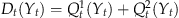 be the total demand (at price p
1, note class 1 customers do not purchase at p
2). Here Y
t
is a random demand parameter, reflecting, for example, weather, exchange rate or other exogenous factors that influence the demand. As naturally demand from different classes can depend differently on those factors, we assume that
be the total demand (at price p
1, note class 1 customers do not purchase at p
2). Here Y
t
is a random demand parameter, reflecting, for example, weather, exchange rate or other exogenous factors that influence the demand. As naturally demand from different classes can depend differently on those factors, we assume that  is a vector of random variables with joint CDF F
Y
(y), defined on a finite, convex set
is a vector of random variables with joint CDF F
Y
(y), defined on a finite, convex set  . Such construct allows us to capture correlations between demand classes; see Appendix S3. We assume
  for all
  in order to avoid trivial cases when all capacity is sold and hence no discounts and learning are possible.
As in other models in the literature, some class 2 customers may wait for a discount that may be offered to attract class 1 customers at the end of the period. In line with earlier works (e.g., Pfeifer 1989), we refer to these diverting customers as “shoppers.” However, a key feature of our model is that their waiting behavior changes over time in response to the firm's decisions. We assume that consumer waiting behavior is described by a waiting parameter, θ t , that represents the propensity of customers to wait for a discount. For example, there could be a random fraction, α t , of class 2 customers waiting and θ t could be the average fraction waiting (this is the construct we use in our simplified models). The waiting parameter θ t changes over time capturing customer learning. We assume that θ t is known at the beginning of period t. The dynamics of the selling period are depicted in Figure 1.
The firm initially sets the price at p
2 and observes the initial sales, S
t
, to class 2 customers. The remainder of class 2 customers, M
t
, are shoppers who wait for a potential discount toward the end of the period; note  . Class 1 customers as per Cachon and Swinney (2009) are “bargain‐hunters”: they do not act strategically and rather all wait and purchase only if price p
1 is offered. The total demand at price p
1 therefore is
. Class 1 customers as per Cachon and Swinney (2009) are “bargain‐hunters”: they do not act strategically and rather all wait and purchase only if price p
1 is offered. The total demand at price p
1 therefore is 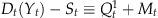 .
.
At a point in time close to the end of period t, denoted as the sale time, the firm determines x
t
, the number of unsold units to put on sale at price p
1, x
t
≥0. If  , then all waiting demand is satisfied and the firm receives revenue of p
2
S
t
+p
1
x
t
and moves to the next period. Otherwise, the firm can receive additional revenue by accommodating the unserved class 2 shoppers as follows.
, then all waiting demand is satisfied and the firm receives revenue of p
2
S
t
+p
1
x
t
and moves to the next period. Otherwise, the firm can receive additional revenue by accommodating the unserved class 2 shoppers as follows.
Let B t (S t , x t , Y t ) be the number of unserved class 2 customers. We assume that once all x t discounted units are sold, the firm again offers units for sale at price p 2 to accommodate unserved class 2 shoppers (or in the three prices extension, section 6, at a higher price p 3). In some industries, for example in airlines, it is common to oversell the capacity, forcing some customers to be “bumped,” i.e., displaced from their seat by another, typically higher‐paying, customer. In such cases with bumping we assume that if B t exceeds the number of unsold units (N−S t −x t ) customers that purchased at a discount are bumped; their units are sold at price p 2 (or p 3 in the three prices model) and the firm incurs a penalty p C per unit bumped. In other industries, for example in cruise lines, only unsold units may be sold at this time. This may occur because of competitive norms, legislation or regulation, or for logistical reasons, such as when a physical object is sold. Letting p C =p 2 (or p 3 in the three prices model) accomplishes this goal as there is no economic justification for overselling. Thus in cases without bumping the potential demand, B t −(N−S t −x t ) is lost.
Observe that there are incentives for class 2 customers to purchase early. Without bumping, class 2 customers may not be served and presumably they would prefer to purchase at p 2 rather than not. With bumping, class 2 customers that purchase a discount seat are subject to bumping. We assume that bumped customers cannot repurchase a unit in the same period—this is a reasonable assumption supported by discussions with travel industry personnel (see model discussion in the supporting information Appendix S1).
The total revenue of the firm net the bumping cost for period t given (S
t
, x
t
, Y
t
) is 
For notational convenience, let  represent the conditional random vector Y
t
having observed S
t
and knowing θ
t
. The expected single‐period revenue in period t is then given by
represent the conditional random vector Y
t
having observed S
t
and knowing θ
t
. The expected single‐period revenue in period t is then given by 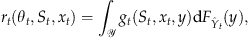
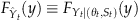 is the CDF of
  .
.
We refer to the two‐vector (θ
t
, S
t
) as the state of the system. We assume that the system evolves based on the decision x
t
according to a function h(θ
t
, x
t
), defining θ
t+1, and a random draw of S
t+1 from the distribution of future sales,  . We refer to h as the learning function because it reflects the changes in the waiting behavior of the customers as they learn about the policy of the firm. We define two types of the learning functions:
smoothing: if
self‐regulating: if
 and
and  , e.g.,
 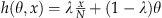 for 0≤λ≤1;
 and
and  , e.g.,
  for
for  .
.
We note that the current literature (e.g., Liu and van Ryzin 2011, Popescu and Wu 2007) considers smoothing dynamics in the parameters of the aggregate demand model. By presenting alternative learning mechanisms, we consider broader cases and derive additional insight; see more discussion about learning behaviors in the supporting information Appendix S1.
The objective of the firm is to maximize the expected T‐period revenue, discounted at a fixed rate δ∈(0, 1). Therefore, the firm determines the number of units on sale, x
t
, for each period t=1, 2, … , T and some initial θ
1, by solving the following dynamic program 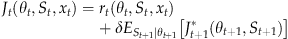
We refer to (3) as the general model, as it expresses the uncertainty in the overall demand as well as in the fraction of class 2 customers waiting in every period. In sections 5.1, 5.3 and 6 we consider simplified models, where one of these uncertainties is removed.
We approach the problem by establishing properties of J
t
(θ
t
, S
t
, x
t
), in particular concavity and supermodularity. To do so, we make several assumptions on the demand and stochastic ordering of the random variables. Specifically, recall that a random variable X with CDF F
X
(x, θ) is said to be stochastically increasing (decreasing, convex, concave, supermodular, etc.) in parameter θ iff 1−F
X
(x, θ) is increasing (decreasing, convex, concave, supermodular, etc.) See sections 2.2 and 3.9.1 in Topkis (1998) as well as Shaked and Shantikumar (1994) for more discussion about stochastic ordering, examples, and applications. We assume that demand function D
t
(Y
t
) is increasing in Y
t
. We assume that (i) S
t
is stochastically decreasing in θ
t
; (ii)  is stochastically increasing in S
t
; and (iii)
is stochastically increasing in S
t
; and (iii)  is stochastically increasing in θ
t
.
is stochastically increasing in θ
t
.
These assumptions are consistent with the following intuitive observations. Because θ
t
measures the propensity of customers to wait, the number of customers who purchase (i.e., do not wait), S
t
, should decrease in θ
t
. Similarly, more customers purchasing at the initial price implies increased  . Defining
  to be increasing in at least one element of Y
t
and not decreasing in any implies
to be increasing in at least one element of Y
t
and not decreasing in any implies  increasing in S
t
. The distribution of the conditional random variable
increasing in S
t
. The distribution of the conditional random variable  is dependent on θ. Upon observation of the same sales, S
t
, any increase in θ would imply greater class 2 demand leading to a (stochastic) increase in
is dependent on θ. Upon observation of the same sales, S
t
, any increase in θ would imply greater class 2 demand leading to a (stochastic) increase in  .
.
For more discussion on the various elements and assumptions of our model (aggregate demand, waiting parameter, bumping, allocation of discounted unit, discount price, and learning behaviors), refer to the supporting information Appendix S1. In what follows we analyze the model; first for the case of self‐regulating learning, and then for smoothing.
For the case of self‐regulating learning, we show that the standard methodologies for establishing concavity, such as Topkis (1998, section 3.9.2), Puterman (1994, section 4.7.3), or their recent extensions (e.g., Smith and McCardle 2002) are not applicable. In their models, the state of the system evolves monotonically in the previous state and decision. That is, the components of the state vector either increase or decrease in the previous state and decision. In our general model (1), state transitions are not monotonic, as S t is stochastically decreasing in θ t , while θ t is increasing in either θ t−1 or x t−1, or both. We therefore develop the necessary methodology and show concavity in section 4.
In section 5, we study the case with a smoothing learning function and show that in general concavity does not hold, unless the speed of customer learning is “slow.” Then we consider two simplifications to the general model and derive their solutions in closed form. Section 6 presents a model with three customer classes.
4. Optimal Policy for Self‐Regulating Learning
In this section, we derive the conditions under which the revenue‐to‐go function is concave when the learning function, h(·), is self‐regulating. Concavity implies that the optimal policy for the firm places some units on sale in each period, relying on the consumer behavior regulating the number of customers waiting.
We organize this section as follows. First in section 4.1 we show that J
t
(θ
t
, S
t
, x
t
) is concave, supermodular, and increasing under that assumption that these properties hold for the single‐period expected revenue function, r(θ, S, x). Then in section 4.2 we discuss the properties of the revenue function  , given in (1) that ensure concavity, supermodularity, and monotonicity of r(θ, S, x). We conclude by presenting an example.
4.1. Concavity in Dynamic Programs with Non‐Monotonic State Transitions
Observe from (3a) that since θ
t+1=h
t
(θ
t
, x
t
) is independent of S
t
, the expected future revenue,  , does not depend on S
t
and therefore, letting
, does not depend on S
t
and therefore, letting  , we can substitute
We make the following four assumptions, which we show hold in the next section. We assume that r
t
(θ
t
, S
t
, x
t
) is (A1) jointly concave in (θ
t
, x
t
), (A2) supermodular in (θ
t
, S
t
, x
t
), (A3) increasing in S
t
, and (A4) S
t
is stochastically concave in θ
t
(and recall that by assumption (i) from section 3 it is also stochastically decreasing in θ
t
). We also make the fundamental assumption of section 4 (A5) h
t
(θ
t
, x
t
) is linear self‐regulating, i.e.,  ,
,  .
.
Concavity and supermodularity in (4) are related by the following lemma (all proofs are presented in the supporting information Appendix S2):
L
Therefore, it is sufficient to show that φ is concave in h, which in our original notation corresponds to  being concave in θ
t
. Observe
being concave in θ
t
. Observe  . Concavity of this integral is established by the following lemma, which extends the only‐if part of Corollary 3.9.1(c) of Topkis (see p. 161) to the case where the integrant depends on the parameter.
L is concave in θ.
As a simple example of a distribution family that satisfies the conditions of the above lemma, consider Uniform[0, a−b θ] for a, b≥0, a−bθ>0. Refer to Shaked and Shantikumar (1994) for further discussion of how to construct random variables with the necessary properties.
Our main result in this section is given by the following theorem.
T
Problem (3) defines a subclass of dynamic programs for which a vector of the system state is not monotonic in the previous period's state and decision. In this section, we have shown how to establish concavity for such dynamic programs. A similar logic with a different set of initial assumptions could be used to prove other properties, for example, convexity. We also note that to our knowledge there is no published research dealing with concavity (convexity) in the dynamic programs with nonmonotonic transitions. As such, this is a technical contribution of our paper.
Next, we discuss the underlying conditions on the customer behavior that ensure concavity.
4.2. Sufficient Conditions for Concavity of J
t
(
θ
t
, S
t
, x
t
)
In this section, we study the properties of  and the other parameters of the model that ensure that the expected single‐period revenue function r(θ, S, x) is concave, supermodular, and increasing, so that by Theorem 1 the revenue‐to‐go, J
t
(θ
t
, S
t
, x
t
), is concave for every period. Since the discussion relates to a single period, time indices are omitted.
and the other parameters of the model that ensure that the expected single‐period revenue function r(θ, S, x) is concave, supermodular, and increasing, so that by Theorem 1 the revenue‐to‐go, J
t
(θ
t
, S
t
, x
t
), is concave for every period. Since the discussion relates to a single period, time indices are omitted.
 determines the number of class 2 “shoppers” who remain waiting once all discounted units are sold. That is, B is the initial number of class 2 shoppers,
  , minus those who bought at a discount, where the latter reflects allocation of discounted units. Therefore B should satisfy the following intuitive conditions. B1:B is increasing in
  and decreasing in S and x; B2:∂B/∂x≥−1; B3:∂B/∂S≥−1; B4: if x≥D(y)−S, then B(S, x, y)=0; and B5:B(S, x, y) is piecewise concave in x on [0, D(y)−S) and [D(y)−S, N].
The increasing/decreasing properties of (B1) follow directly from the definition. Conditions (B2) and (B3) hold because the discounted units are allocated between class 1 and 2 customers: if additional Δ discounted units are available, some of them will be sold to class 1 customers, and so the number of class 2 customers remaining can decrease by at most Δ, and similarly, if additional Δ class 2 customers purchased early, then the chances of waiting class 2 customers to obtain discounted units decrease (because the number of class 1 customers does not change), thus the number of unserved class 2 customers decreases by at most Δ. (B4) implies if sufficient capacity is available to accommodate all customers, then no customers remain. Finally, (B5) implies the rate of decrease in the number of unsatisfied customers (weakly) increases with the number of discounted units, e.g., as would be the case if units are allocated randomly. In addition to assumption (ii) that  is stochastically increasing, we also assume that
  is stochastically concave in S and θ, and stochastically supermodular in (θ, S). These additional assumptions hold until the end of this section. We have the following lemmas:
L
L for all
 or if
or if
 .
.
Lemma 4 implies that if there is always sufficient demand to fill the capacity the revenue function is concave. Otherwise, the assumption ∂B/∂x≥−p
1/p
2 implies that for a Δ increase in x, at most p
1/p
2 × 100% is allocated to class 2 customers and (1−p
1/p
2) × 100% goes to class 1. For example, if discounted inventory is allocated in proportion to demand, the ratio of class 1 to class 2 customers should be greater than (p
2−p
1)/p
2. If demand is low and ∂B/∂x<−p
1/p
2, then for each additional unit of x, the additional sales at the lower price cannibalize too much of the revenue from the waiting class 2 customers. In this case, offering no discounts is optimal, though concavity in the expected revenue cannot be assured. We note that concavity of r(θ, S, x) in x could hold in this case if the distribution of  places sufficiently small probability on
  .
.
The optimal number of units on sale in the single period can be determined by solving the first‐order condition \xE2\x88\x82r(θ, S, x)/∂x=0, and is given by the following corollary:
C , satisfies
Recalling ∂B/∂x<0, the first‐order condition implies x should be chosen to balance the marginal additional revenue gained from bargain‐hunters (class 1) less the marginal diverted revenue from class 2 customers who purchase at p
1 with the marginal penalty costs less the penalty costs saved by serving additional class 2 customers. That is, (5) expresses the newsvendor‐like balance: 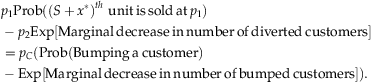
Joint concavity and supermodularity of r(θ, S, x) are discussed in the following lemma:
L for all
 in the support of
 and
and
 ; or (ii)
 for all
 in the support of
 , and
, and
 .
.
Summarizing, we have the following theorem:
T
As an example of a function that satisfies the assumptions, suppose that demands from class 1 and 2 customers are given by multiplying nominal demands, d
1 and d
2, by a random variable, Y. Demand at price p
2 is yd
2 and at price p
1 is y(d
1+d
2). Let  be the minimum value of the support of Y. For the case with p
C
=0 and
be the minimum value of the support of Y. For the case with p
C
=0 and  , consider
  . Here, the number of remaining class 2 customers reflects the total number of class 2 customers that wait,
  , net the number of class 2 customers that purchased product at the end‐of‐period sale. Further, the discounted units are allocated on proportion, which is constant and depends on the nominal demands, d
2/(d
1+d
2). With this,
, net the number of class 2 customers that purchased product at the end‐of‐period sale. Further, the discounted units are allocated on proportion, which is constant and depends on the nominal demands, d
2/(d
1+d
2). With this, 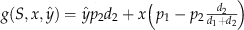 , which is supermodular in
  , and linear in
  . Therefore, the conditions of Theorem 2 hold and the expected revenue‐to‐go function is concave for every period, and so the optimal number of units on sale is easy to find.
Our results also suggest a neat interpretation of the optimal policy for the case with self‐regulating learning. First, concavity implies that the firm places some units on sale in every period. Furthermore, since the revenue function is supermodular, the number of units on sale increases in the waiting parameter. But, the self‐regulating learning behavior controls the number of customers waiting in the subsequent period so that it does not continue to increase. The firm takes a passive role, placing some units on sale, and relying on the consumer behavior to control future waiting. This is not the case for smoothing learning functions, where the firm must actively manage consumer waiting as we discuss below.
5. Optimal Policy for Smoothing Learning Function
In this section, we assume that the learning function h
t
(θ
t
, x
t
) is smoothing; that is, the next period's waiting parameter, θ
t+1, increases in both the current waiting parameter, θ
t
, and the number of units on sale in period t, x
t
. We show that in the general model the revenue‐to‐go function is not necessarily concave, unless the speed of consumer learning is “slow” as defined below. To address the problems with arbitrary speed of learning, we present two simplified models and show that for either simplification, the optimal policy has a “bang–bang” structure where the firm alternately places a number,  , or zero units on sale. We describe this optimal policy in the closed form.
Under the assumption that the learning function is linear, concavity and supermodularity of the revenue‐to‐go require, respectively: 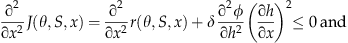
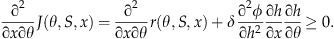
Because smoothing learning implies  , for (6) and (7) to hold when r is concave and supermodular, we must place some restrictions on the curvature of φ(h(θ, x)).
3
Specifically, observe that ∂h/∂x reflects the speed at which customers learn about the firm's decisions. If r is concave, then from (6) if ∂h/∂x is small enough then J would be also concave.
, for (6) and (7) to hold when r is concave and supermodular, we must place some restrictions on the curvature of φ(h(θ, x)).
3
Specifically, observe that ∂h/∂x reflects the speed at which customers learn about the firm's decisions. If r is concave, then from (6) if ∂h/∂x is small enough then J would be also concave.
Slow learning has been documented in the works on reference price learning with respect to the sales promotions. Greenleaf (1995) and Hardie et al. (1993) studied point‐of‐sales data for such commodities as peanut butter and refrigerated orange juice, and reported an analog of our ∂h/∂x to be at 0.075 and 0.17, respectively. However, we know of no research regarding the speed of learning for discounts in services. This is of interest for future research.
The speed of learning also plays an important role in Gallego et al. (2008) and Liu and van Ryzin (2011). Specifically, in the former, numerical simulations suggest that in the case of slow learning, the firm should offer a constant number of units on sale, and otherwise the number should be raised and lowered in alternate periods. Next, we prove a similar result analytically and provide a closed form expression for the number of units on sale.
5.1. Simplified Models
In this section, we simplify the general model so that upon observing the initial sales, the firm can infer the exact number of customers waiting for period t. The future demand and purchasing behavior remain stochastic. This simplification allows us to solve the problem in the closed form while utilizing a less constrained B(S, x, y) and relaxing the linearity assumption of the learning function.
For the remainder of the paper, let  be a random variable and let demand from each class reflect a nominal demand, d
i
, i=1, 2 multiplied by Y. For class 2, demand is d
2
Y
t
and for class 1, demand is d
1(a+bY
t
), where a, b are given constants. Observe that with b>0 class 1 and 2 demands are positively correlated, with b<0 then are negatively correlated, and for a>0, b=0 class 1 demand is a constant. Note that in the two former cases demands are perfectly correlated. An extension to the nonperfectly correlated demands is presented in the supporting information Appendix S3. With these, the total demand from both classes is D
t
(Y
t
)=Y
t
d
2+(a+bY
t
)d
1. We assume
be a random variable and let demand from each class reflect a nominal demand, d
i
, i=1, 2 multiplied by Y. For class 2, demand is d
2
Y
t
and for class 1, demand is d
1(a+bY
t
), where a, b are given constants. Observe that with b>0 class 1 and 2 demands are positively correlated, with b<0 then are negatively correlated, and for a>0, b=0 class 1 demand is a constant. Note that in the two former cases demands are perfectly correlated. An extension to the nonperfectly correlated demands is presented in the supporting information Appendix S3. With these, the total demand from both classes is D
t
(Y
t
)=Y
t
d
2+(a+bY
t
)d
1. We assume  and d
2+bd
1≥0 to ensure that D is increasing in Y.
and d
2+bd
1≥0 to ensure that D is increasing in Y.
Let  be the fraction of the class 2 demand that waits for the end‐of‐period sale in period t. We refer to α
t
as the waiting fraction. Observe that M
t
=α
t
Y
t
d
2 and S
t
=(1−α
t
)Y
t
d
2.
be the fraction of the class 2 demand that waits for the end‐of‐period sale in period t. We refer to α
t
as the waiting fraction. Observe that M
t
=α
t
Y
t
d
2 and S
t
=(1−α
t
)Y
t
d
2.
In this section, we consider two simplifications:
Deterministic waiting fraction model: in which the demand multiplier, Y
t
, is stochastic, but its distribution does not depend on the waiting parameter; the waiting fraction is deterministic with α
t
≡θ
t
, and evolves according to a smoothing concave learning function α
t+1=h
t
(α
t
, x
t
);
Deterministic demand model: in which Y
t
≡Constant for all t=1, 2, … , T and w.l.o.g. we set Y
t
≡1; the random waiting fraction, α
t
, is stochastically increasing and concave in the waiting parameter θ
t
, which evolves according to a smoothing concave learning function θ
t+1=h
t
(θ
t
, x
t
).
Let A
t
(α
t
, Y
t
) be the actual demand for the discounted seats. A
t
(α
t
, Y
t
)=D
t
(Y
t
)−S
t
=ad
1+Y
t
(d
2+bd
1)−S
t
. Since the firm puts x
t
units on the end‐of‐period sale, min[x
t
, A
t
] units are sold at the discounted price p
1. Assuming that the discounted inventory is allocated proportionally between class 1 and class 2 customers based on their realized demands, the number of class 2 customers that purchase discounted units is 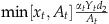 . The number of unserved class 2 customers after the sale is
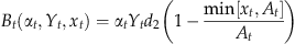
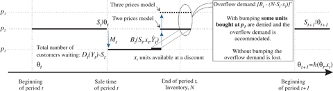
Observe that for either simplified model by knowing θ t and observing S t the firm can determine the exact (realized) values for α t and y t , and therefore at the sale time there is no uncertainty for the current period. If A t +S t =D(y t )<N, then the firm has excess capacity and bumping cannot occur. Otherwise the capacity is scarce, and bumping can occur if too many units are put on sale.
Since the firm knows which case realizes with certainty, it forces an intuitive restriction p C ≥p 1. Otherwise firms could intentionally sell discounted products and later bump class 1 customers (as overflow) for a premium of p 1−p C >0.
5.2. Single‐Period Solution for the Simplified Models
Let  be the maximum number of discounted units such that (i) all class 2 customers are allocated a product without bumping others; and (ii) all
  units are sold. In the case of excess capacity, the firm cannot sell all available inventory, and so
  . For the scarce capacity case, solving
 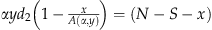 yields
  . Observe
  . In summary,
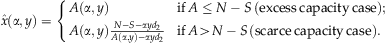
T , such that if
 then
then
 . Otherwise, in the case of scarce capacity,
  , and in the case of excess capacity any
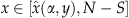 is optimal.
We note that  if D
t
(Y
t
)p
1≤Y
t
d
2
p
2. That is,
if D
t
(Y
t
)p
1≤Y
t
d
2
p
2. That is,  if the potential revenue at price p
2 exceeds the potential revenue at p
1. In this case, the single‐period optimal policy is “bang–bang”: the optimal number of discounted units drops down to zero if too many customers wait (i.e., when
if the potential revenue at price p
2 exceeds the potential revenue at p
1. In this case, the single‐period optimal policy is “bang–bang”: the optimal number of discounted units drops down to zero if too many customers wait (i.e., when  ); and it jumps up to
  otherwise. In the opposite case, if
  , then α is always smaller than
  and some number of units are always placed on a discount. Next we prove that a similar “bang–bang” policy holds for every period.
5.3. Multiple‐Period Solution for Simplified Models
Let R
t
(θ
t
, α
t
, y
t
, x
t
) be the expected revenue‐to‐go, given that for period t, the waiting parameter is θ
t
, the realized waiting fraction is α
t
, the observed demand multiplier is y
t
and x
t
units are put on sale. The optimal number of discounted units,  , can be found for each period, t=1, 2, … , T, by solving the following dynamic program:
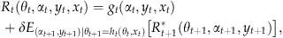

 for all (θT
+1, αT
+1, yT
+1); and θ
t+1=h
t
(θ
t
, x
t
) is increasing and concave in either argument. Because θ
t+1=h
t
(θ
t
, x
t
) does not depend on the realized values of α
t
and y
t
, we can write R
t
(θ
t
, α
t
, y
t
, x
t
)=g
t
(α
t
, y
t
, x
t
)+δφ
t+1(h
t
(θ
t
, x
t
)). In our two simplified models, φ
t+1 takes the following specific forms:
for all (θT
+1, αT
+1, yT
+1); and θ
t+1=h
t
(θ
t
, x
t
) is increasing and concave in either argument. Because θ
t+1=h
t
(θ
t
, x
t
) does not depend on the realized values of α
t
and y
t
, we can write R
t
(θ
t
, α
t
, y
t
, x
t
)=g
t
(α
t
, y
t
, x
t
)+δφ
t+1(h
t
(θ
t
, x
t
)). In our two simplified models, φ
t+1 takes the following specific forms:
In the deterministic waiting fraction (DW) model, α
t
≡θ
t
for all t by assumption and the distribution of Y
t
is independent of α
t
. Therefore,
In the deterministic demand (DD) model, Y
t
≡1 for all t by assumption, and so w.l.o.g. y can be dropped from the expectation of the future revenue, leading to


Let  be the set of “potentially optimal” solutions for period t. Our main result for the simplified models is that
  for all t=1, 2, … , T. The concept of our proof is the following. Suppose that the expected future revenue, φ
t+1, is decreasing and convex in x
t
and α
t
. Since g
t
(α
t
, x
t
, y
t
) is piecewise linear in x, R
t
consists of two adjacent and convex segments. Since g is also decreasing for
for all t=1, 2, … , T. The concept of our proof is the following. Suppose that the expected future revenue, φ
t+1, is decreasing and convex in x
t
and α
t
. Since g
t
(α
t
, x
t
, y
t
) is piecewise linear in x, R
t
consists of two adjacent and convex segments. Since g is also decreasing for  , R
t
is also decreasing if
, R
t
is also decreasing if  . Therefore,
 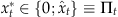 . We summarize this result in the theorem below.
T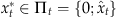 for all periods t=1, 2, … , T.
To summarize, for the case with a smoothing learning function for both simplified models, the optimal policy is “bang–bang”; it places either 0 or  units on the end‐of‐period sale depending on the realized waiting fraction, α
t
. The firm increases the number of “shoppers” by offering units on sale, and then withdraws revenue from those shoppers by periodically not offering any discounted units, subsequently decreasing the likelihood of future waiting.
units on the end‐of‐period sale depending on the realized waiting fraction, α
t
. The firm increases the number of “shoppers” by offering units on sale, and then withdraws revenue from those shoppers by periodically not offering any discounted units, subsequently decreasing the likelihood of future waiting.
By following such policy, the firm simultaneously achieves high utilization of its capacity and controls the number of customers waiting. This policy is quite different from that of the self‐regulating case, because the firm actively manages the waiting, as opposed to relying on the consumers to regulate the waiting themselves. Observe that since  bumping is never optimal. This is because the marginal revenue p
2 per unit could as well be obtained from the initial sales, and since the future revenue is decreasing in x
t
, the firm puts fewer units on sale and reduces the future waiting. This is not the case if the firm can obtain a marginal revenue in excess of p
2, as happens in the three‐price model that we study next.
bumping is never optimal. This is because the marginal revenue p
2 per unit could as well be obtained from the initial sales, and since the future revenue is decreasing in x
t
, the firm puts fewer units on sale and reduces the future waiting. This is not the case if the firm can obtain a marginal revenue in excess of p
2, as happens in the three‐price model that we study next.
6. Three‐Price Model
Next we study the case where a firm may choose to offer some units for sale at p 1, while raising the price to a higher value for the remaining inventory. By doing so the firm can both capture the low‐price demand, as well as the demand willing to pay extra for being accommodated after all discounted units are already sold. The three‐price model reflects frequently observed situations where the “walk‐up” price is higher than the regular, while some units have been sold at a discount earlier.
Let p
3≥p
2 be the “high” price. We build up on the simplified model of section 5.1 amended as follows. We assume only class 3 customers are willing to purchase at price p
3 and let their demand in period t be Y
t
d
3≡Y
t
D
3. The number of customers who are willing to pay price p
2 is now Y
t
D
2, where D
2=d
2+d
3. Also let D
1=d
1+d
2+d
3. We assume  as before. At the sale time the firm decides x
t
, the number of units to offer at the discounted price p
1. The remaining units are offered at price p
3.
as before. At the sale time the firm decides x
t
, the number of units to offer at the discounted price p
1. The remaining units are offered at price p
3.
To determine the revenue of the firm, S
t
≡(1−α
t
)Y
t
D
2 units are sold at the initial price p
2, and min[x
t
, A
t
] units are sold at the discounted price p
1, where A
t
≡(a+bY
t
)d
1+α
t
Y
t
D
2. Let ψ
t
(α
t
)∈[0, 1] be the fraction of class 3 customers who wait for a discount, given that there is a fraction  of class 2 and 3 customers waiting combined. That is, the total number of class 3 customers waiting is ψ
t
(α
t
)Y
t
d
3, and the number of class 2 customers is αY
t
D
2−ψ
t
(α
t
)Y
t
d
3. Since the latter is non‐negative, it is implied that ψ
t
(α
t
)Y
t
d
3≤αY
t
D
2 for all
of class 2 and 3 customers waiting combined. That is, the total number of class 3 customers waiting is ψ
t
(α
t
)Y
t
d
3, and the number of class 2 customers is αY
t
D
2−ψ
t
(α
t
)Y
t
d
3. Since the latter is non‐negative, it is implied that ψ
t
(α
t
)Y
t
d
3≤αY
t
D
2 for all  .
.
As before, we assume that the discounted units are allocated on proportion. That is, the number of discounted units that are sold to class 3 customers is 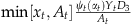 and the net single‐period revenue is
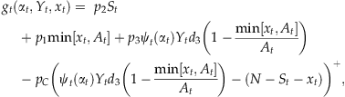
In this section, we assume that the demand multiplier, Y t , is stochastic, and the waiting fraction, α t , is deterministic. 4 We assume that the distribution of Y t does not depend on α t , and that in turn, α t evolves according to a linear learning function α t+1=h t (α t , x t ). We place no restriction whether h(·) is smoothing or self‐regulating.
In order to proceed we need to further specify the properties of ψ(α). Consider the case where it is the firm's policy not to oversell capacity and subsequently lose unsatisfied customer demand (the “no‐bumping” case). Because class 3 customers have a higher valuation for the product, they are less willing to wait and risk not receiving a unit. Therefore, we assume ψ is “small,” compared with α, and class 3 customers do not wait unless many class 2 customers are already waiting. For example, if we assume that class 3 customers do not wait, unless all class 2 customers are already waiting, then 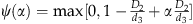 for α∈[0, 1].
In the case where the firm is willing to bump passengers (the “bumping” case), class 3 customers who waited but did not get a discounted unit do not have capacity concerns, as they are guaranteed a product at their reservation price, p
3 (since  ). Therefore, they are more likely to wait, and we assume ψ is “large”; there may be a fraction of class 3 customers waiting even if no class 2 customers wait. For example, if
  for
for 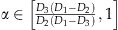 , the fraction of class 3 customers that always wait is
  .
.
We assume that ψ is non‐decreasing convex. In the no‐bumping case ψ=0 for  for some
  and ψ′D
3=D
2, otherwise. In the bumping case, ψ′D
3≤D
2 and ψ′A(α, y)≤ψyD
2. Functions that satisfy these assumptions correspond to the “small” and “large” ψ as per the discussion above.
and ψ′D
3=D
2, otherwise. In the bumping case, ψ′D
3≤D
2 and ψ′A(α, y)≤ψyD
2. Functions that satisfy these assumptions correspond to the “small” and “large” ψ as per the discussion above.
We redefine  to include the waiting of class 3 customers as follows:
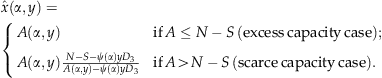
By the same argument as in the proof of Theorem 3, we obtain that the single‐period optimal policy resembles that of the two‐price model.
T , such that if
 , then
  in the case of scarce capacity, and any
 is optimal in the case of excess capacity. Otherwise,
  .
.
In this case,  if D
t
(Y
t
)p
1≤Y
t
D
3
p
3. That is, if the revenue from the high‐price segment exceeds the revenue from all segments at the low price, then the single‐period optimal policy is “bang–bang.” For multiple periods the result extends as follows:
if D
t
(Y
t
)p
1≤Y
t
D
3
p
3. That is, if the revenue from the high‐price segment exceeds the revenue from all segments at the low price, then the single‐period optimal policy is “bang–bang.” For multiple periods the result extends as follows:
T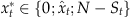 , and without bumping
 for all periods t=1, 2, … , T.
In sum, the optimal policy follows a pattern similar to that of the two‐class model: increasing the fraction of customers waiting by offering units on sale followed by periods where no units are discounted. By doing so, the firm can withdraw revenue from waiting class 3 customers while decreasing future waiting. There is, however, a major difference between the two‐ and three‐price models. In the former, even if the firm's policy was to bump customers if overflow occurs, doing so was never optimal. In contrast, in the latter, the optimal solution could involve selling all of the available N−S units at p 1, bumping some customers, and paying penalty p C <p 3. By doing so the firm can encourage more class 3 customers to wait, and potentially get revenue p 3 in excess of the regular price p 2 per unit, even though it may result in paying bumping penalties.
7. Numerical Studies
In this section, we provide several examples to illustrate the value of making decisions optimally as compared with several heuristics managers use in real‐life situations, and examine how this value and the optimal policy itself change in different situations. We also analyze how to select the optimal discount price  . We use the three‐price model because it allows for all types of consumer behavior that we study in our paper. We consider the case with positively correlated demands (i.e., with a=0, b=1 leading to the class 1 demand of Y
t
d
1).
. We use the three‐price model because it allows for all types of consumer behavior that we study in our paper. We consider the case with positively correlated demands (i.e., with a=0, b=1 leading to the class 1 demand of Y
t
d
1).
We set N=100, δ=0.95, D 2=50, p 1=100, p 2=300, and p 3=500, and consider four families of instances: smoothing bumping (MB), smoothing no‐bumping (MN), self‐regulating bumping (RB), and self‐regulating no‐bumping (RN). For each family of instances we study four demand curves, with D 1=150 or D 1=100, and D 3=30 or D 3=10 for class 3 customers. We denote these demand curves as “150–50–30,” “150–50–10,” “100–50–30,” and “100–50–10,” respectively. For cases with bumping we study two penalties: p C =150 and p C =450.
We use functions 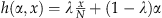 and
and  for 0<λ<1 for the smoothing and self‐regulating learning, respectively. We use
 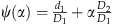 and
and 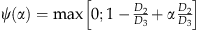 for waiting functions with and without bumping, respectively.
We set  and
and  , so that the demand multiplier Y
t
∈[0.6, 1.4], and examine three distributions: truncated Normal[1, 0.2],
5
Beta[1.75, 3], and Beta[0.8, 2], with the expected values and CVs, respectively (1, 0.913, 0.841) and (0.181, 0.191, 0.237). The results are very similar and below we report only the case with Beta(0.8;2).
, so that the demand multiplier Y
t
∈[0.6, 1.4], and examine three distributions: truncated Normal[1, 0.2],
5
Beta[1.75, 3], and Beta[0.8, 2], with the expected values and CVs, respectively (1, 0.913, 0.841) and (0.181, 0.191, 0.237). The results are very similar and below we report only the case with Beta(0.8;2).
For each instance we compute the expected infinite horizon discounted revenue (the revenue), assuming that the system starts from steady state—intuitively, this is the revenue that the firm will generate starting at an arbitrary time in the future. To compute the revenue we discretize α t as {0; 0.01; 0.02; … ; 1} and discretize y t as {0.6; 0.7; … ; 1.4} for a total of 909 states. We use successive approximations with error bounds to compute the infinite horizon expected revenue function value (Bertsekas 1987, pp. 188–193). Then, we determine the subset of recurrent states and the steady state probabilities, and obtain the expected revenue as the weighted sum (Puterman 1994, pp. 589–594).
In Figure 2a, we present a sample path for the optimal decision,  , and the fraction of customers waiting, α
t
, and in (b) we present the recurrent states and the frequencies with which they are visited in the steady state. We observe that the optimal decision and the fraction of customers waiting follow the cycles of variable length. This expresses the “bang–bang” structure of the optimal policy: if in period t the fraction of waiting customers, α
t
, gets large enough, then the firm puts
, and the fraction of customers waiting, α
t
, and in (b) we present the recurrent states and the frequencies with which they are visited in the steady state. We observe that the optimal decision and the fraction of customers waiting follow the cycles of variable length. This expresses the “bang–bang” structure of the optimal policy: if in period t the fraction of waiting customers, α
t
, gets large enough, then the firm puts  units on sale and so α
t+1 drops. Hence in period t+1 the firm puts
units on sale and so α
t+1 drops. Hence in period t+1 the firm puts  units on sale and α
t+2 increases again; note the 1‐period time lag between x and α in (a). Following such cycles, the optimal policy visits a variety of states; see (b). Because of the uncertainty in demand, the length of cycles is random. Thus, the customers cannot anticipate the transitions and hence the decision of the firm.
units on sale and α
t+2 increases again; note the 1‐period time lag between x and α in (a). Following such cycles, the optimal policy visits a variety of states; see (b). Because of the uncertainty in demand, the length of cycles is random. Thus, the customers cannot anticipate the transitions and hence the decision of the firm.

,
7.1. Performance of the Optimal Policy and Managerial Insights
To better understand the performance of the optimal policy, we compare it with four heuristics that appeal to managers. In each heuristic we determine the number of units to put on sale through different methods. We consider the following:
Do‐nothing: Let x t =N−S t or x t =0 for all t, whichever is better.
BestP: Let x
t
=N−S
t
with probability  and x
t
=0 with probability
and x
t
=0 with probability  , where the value of
  is the one that results in the highest revenue.
S
*: Let x
t
=N−S if  and x
t
=0, otherwise, where the value of
and x
t
=0, otherwise, where the value of  is the one that results in the highest revenue.
Beta
*: Let x
t
=N−S
t
with probability  , and x
t
=0 with probability
, and x
t
=0 with probability  , where the value of
  is the one that results in the highest revenue.
The rationale behind the do‐nothing heuristic is straightforward: choose the better of “all” or “none” on sale and do so consistently in all periods. The BestP heuristic attempts to prevent consumers from guessing if a sale will occur in a given period.
6
Heuristics S
* and Beta* represent a nave managerial approach where discounts are offered in periods with low regular price sales (i.e., when S
t
is small). The former heuristic does so when a threshold is crossed, whereas the latter places units on sale based on a linear probabilistic rule. We find  ,
,  , and
, and  through numerical search. Given the revenues of the optimal and heuristic policies, we compute the relative improvement of the optimal policy over a particular heuristic as (optimal revenue−heuristic revenue)÷(heuristic revenue).
Figure 3 presents the relative improvements over the heuristics for the four families of instances with 150–50–30 demand curve and Beta(0.8;2) demand multipliers. Our main observation is that in all cases the optimal policy generates 5–15% additional revenue over the best heuristic. This value changes depending on the speed of learning and the type of consumer behavior. It also depends on which heuristic is the best.
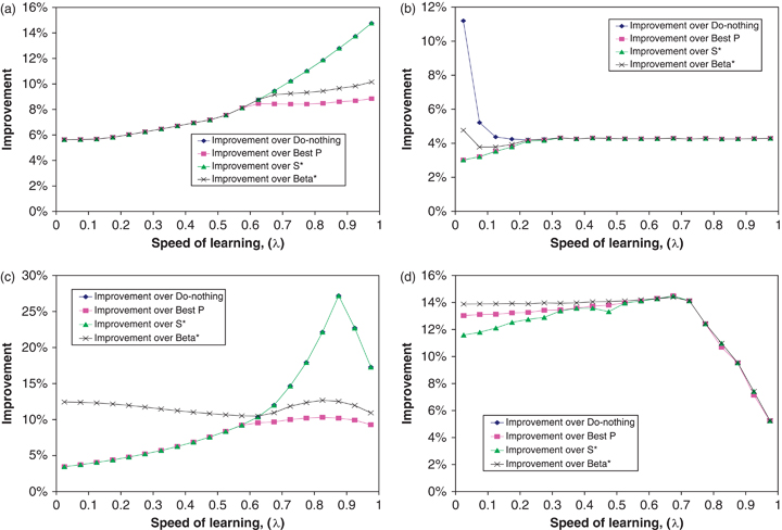
In the cases without bumping (Figure 3a and c), the best heuristic is BestP, as it outperforms heuristics S
* and Beta*. At a first glance this might seem slightly counterintuitive, since the latter are based on the intuitive managerial approach to put more units on sale when S
t
is small. However, recall that the optimal policy suggests exactly the opposite to this nave approach. Specifically,  if
if  , and since S
t
=(1−α
t
)y
t
D
2, it follows that (in expectation) it is optimal not to put units on sale in the periods with small S
t
.
, and since S
t
=(1−α
t
)y
t
D
2, it follows that (in expectation) it is optimal not to put units on sale in the periods with small S
t
.
The improvement over the BestP heuristic depends on the speed of learning. This is because the optimal policy determines when to offer a discount (the timing), and if one is offered, then how many units to discount (the number). By choosing the best probability, the BestP heuristic “optimizes” the long‐run average number of units on sale, but cannot achieve the right timing of sales. In the cases of slow learning in order to change waiting behavior, the firm must have consistent series of periods with and without discounts. The BestP heuristic cannot ensure such consistency, and therefore chooses to do nothing (indeed  for λ<0.625 on Figure 3a and for λ<0.575 on Figure 3c). For faster speeds of learning, consistency is not required as customers readily change their waiting behavior; therefore the timing of sales is less important than the average number of units on sale.
In the instances with bumping (Figure 3b and d), the best heuristic is S *. This is because even though all heuristics bump customers in the situations where the optimal policy does not, S * bumps the least. As discussed above, the S * heuristic has a direct control over the timing, as opposed to the probabilistic heuristics, which do not. Better timing implies less frequent bumping and consequently lower (total) bumping penalty, so the S * heuristic returns higher revenue in the cases with bumping than other heuristics. Also, because the total penalty is proportional to p C , the improvement is naturally larger in the cases with large p C : compare (b) and (d) in Figure 3.
Next, we study the factors that influence whether strategic revenue management as we discuss in this paper will be effective. Table 1 classifies different instances into those where the firm benefits from offering end‐of‐period discounts and those where it does not. In the cases with few class 3 customers (rows 1 and 2 in Table 1), observe that discounts increase revenue only in the cases with bumping. This is because if the firm bumps customers to accommodate class 3 overflow, then it provides an incentive for more class 3 customers to wait (through the ψ(α) function). But because there are few class 3 customers overall, the number of waiting class 3 customers is still small compared with the number of class 1 customers. As a result, only a few class 3 customers who wait are able to buy at a discount, while most buy at p 3, hence increasing firm's revenue. In contrast, when there are many class 3 customers and few class 1 customers (row 3), the threat imposed by refusing to bump customers forces fewer high‐value class 3 customers to wait (through ψ(α)), allowing the firm to sell much of its capacity early at price p 2 and gain revenue by offering discounts that are mostly purchased by class 1 customers. Without the threat (i.e., with bumping) the reaction function ψ(α) changes and too many class 3 customers wait and purchase discount seats, instead of purchasing them early at price p 2. Thus, given a choice, depending on the relative class 1 and class 3 demand, the firm may or may not prefer to oversell its capacity and bump passengers. That is, the firm can use bumping strategically to induce appropriate customer behavior and enhance the effectiveness of its revenue management policy.
7.2. Selecting the Optimal Discount Price, 
Our model assumes that the discount price, p
1, is fixed for the entire horizon of T periods, and as we argue in the introduction, building a model where customers react to both price and availability of discounted units is nontrivial. As research in dynamic pricing shows, however, a heuristic that charges an optimally selected single price (as opposed to optimizing it dynamically) often performs only marginally suboptimally (Gallego and van Ryzin 1994). Therefore, as a heuristic policy, the firm could search for the optimal “static” discounted price,  , charge it in every period, and then determine the number of discounted units to put on sale following our optimal policy.
We search for such optimal static price,  , numerically over its domain, [0, p
2]; see Figure 4. In this example, we impose a demand curve D(p)=200−0.5p (so that D(300)=50 and D(100)=150 as in previous examples). We also assume that the value of a discount influences the rate at which customers are willing to change their behavior, i.e., the speed of learning. In particular, we assume λ(p)=0.3−0.001p. We experimented with other functions for demand and speed of learning, but observed no qualitative differences from the case presented (see Figure 4).
, numerically over its domain, [0, p
2]; see Figure 4. In this example, we impose a demand curve D(p)=200−0.5p (so that D(300)=50 and D(100)=150 as in previous examples). We also assume that the value of a discount influences the rate at which customers are willing to change their behavior, i.e., the speed of learning. In particular, we assume λ(p)=0.3−0.001p. We experimented with other functions for demand and speed of learning, but observed no qualitative differences from the case presented (see Figure 4).
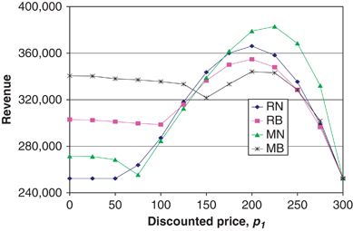
Two observations are evident from Figure 4. First, the revenue is not concave and often not quasiconcave in the price, therefore it may not be possible to determine the optimal discount analytically. There is an obvious optimal point, however. Such a point exists because the firm uses class 1 demand to achieve two goals. On one hand it wants p 1 to be high, because then it obtains larger revenue from the sale of each discounted unit. On the other hand, it wants D(p 1) to be high, because under proportional allocation class 1 customers displace some waiting class 3 customers, so that they purchase at the higher price, p 3. Since price negatively affects demand, these goals conflict and an optimal trade‐off point is found.
Figure 4 also provides a neat illustration to the earlier point that firms can strategically use bumping to increase revenue. Observe that when the discounted price is small, hence, class 1 demand is high, more revenue is obtained when the firm bumps passengers (RB and MB curves are higher than RN and MN). Conversely, when the price is large, class 1 demand is small, and the firm benefits from not bumping (RN and MN curves are higher).
8. Conclusions
Our work is motivated by the concern that given the increased ability to search for better prices for travel‐related products (flights, vacation packages, etc.), consumers will learn to expect end‐of‐period deals and will strategically wait for them. We study the problem for cases of two and three customer classes. The two‐class problem represents the case where a list price is given (as in the cruise or vacation packages industries); the three‐class problem reflects typical airline pricing where prices may decrease or increase in the days before departure. We formulate the problem as a dynamic program and develop a unique solution approach amenable to the novel structural properties we find in the problem.
For the case of two customer classes with self‐regulating customer behavior, we show that the firm in general will set some units on sale in each period and allow the customer behavior to limit the number receiving the benefit of the reduced price inventory. In contrast, in the case of smoothing customer behavior, we show the firm should follow a “bang–bang” sale policy, either placing most of the remaining units on sale or none. Thus, the firm takes a more active role, adjusting the customers' expectations by alternately increasing the number of customers waiting until a threshold is crossed, upon which the firm places no units on sale. By doing so, the firm is able to regulate the number of customers waiting and to increase its revenue by increasing utilization, allowing some units that would otherwise not be sold to be purchased by the lower‐value customers.
In the model with three customer classes, we consider how high‐value customers react to a firm's bumping policy. In the cases with bumping, high‐value customers have a higher incentive to wait. As a result, in addition to the “bang–bang” policy, it could be optimal to discount all units remaining and pay bumping penalty. Such policy, however, is beneficial only if there are few high‐value customers. Establishing a policy of not bumping passengers is beneficial when there are many high‐value customers. Overall, the benefit from following the optimal policy is 5–15% more revenue as compared with several intuitive managerial heuristics.
We acknowledge that the model formulated here does not account for all factors that may influence strategic customer behavior in revenue management. Future studies should consider more explicit formulations of customer utility, competition between firms and gaming by both firms and customers. In addition, empirical work is needed to better understand consumer learning behavior with regards to travel‐related discounts.
Footnotes
1
Source: private conversation with a manager at a leading revenue management software firm.
2
This is a technical condition required to interchange differentiation and integration in the proof of the Lemma. As needed, we assume all intervals/sets are Borel sets and all functions are Borel measurable and integrable with respect to an appropriately defined probability triple.
3
Remark: This was not necessary in the case with self‐regulating learning because in that case and so when r and φ are concave, concavity and supermodularity of J also follow.
4
Alternative models with stochastic demand and waiting, or deterministic Y and stochastic α, could in general be of interest as well. However, we found that in three‐price context they place restrictive and uninterpretable conditions on prices, demands, and waiting. Therefore we do not present them.
5
We use 2σ limits so that the endpoints have non‐negligible probabilities.
6
A variation of the BestP heuristic is used by a car rental company with whom we discussed our work: they have a deal almost every week, but to access it, customers need a promotion code. These codes are e‐mailed to a subset of their registered webmail customers, where a customer is included on the mailing list for a given week with some probability.