Dynamic Pricing in the Presence of Myopic and Strategic Consumers: Theory and Experiment

Abstract

We investigate retailers’ dynamic pricing decisions in a stylized two‐period setting with possible supply constraints and demand from both myopic and strategic consumers. We present an analytical model and then test its predictions in a behavioral experiment in which human subjects played the role of pricing managers. We find that the fraction of strategic consumers in the market systematically moderates the optimal pricing structure. When this fraction exceeds a certain threshold, the retailer offers relatively small late season markdowns to discourage strategic consumers from waiting and to incentivize them to buy during the early season; otherwise, the retailer offers relatively large markdowns to divert all strategic consumers to the late season, where the majority of revenue is made. Our model analyses suggest that the latter policy is optimal under fairly broad conditions. Our experiment shows that after some significant learning, aggregate behavior is able to approximate the key qualitative predictions from our model analysis, with one notable deviation: in the presence of a mixture of myopic and strategic consumers, subjects act somewhat myopically – they underprice and oversell in the main selling season, which significantly limits their ability to generate revenue in the markdown season.

Keywords

dynamic pricing inventory scarcity myopic consumers strategic consumers

Introduction

Dynamic pricing and revenue management techniques have been a notable success in many industries. Despite the progress in automation of pricing decisions, however, actual pricing decisions are often made by managers. For example, Phillips ( 2005) writes that “In most stores, buyers were responsible for ... setting list prices, and planning promotions and markdowns.” Echoing this statement, as an executive at a major retail chain pointed to us, the pricing tool that is most commonly used in practice is “a meeting,” implying that people and not automated systems are often responsible for pricing decisions. Overall, pricing is difficult for managers (Dolan 1995), but in recent years, due to the proliferation of markdowns, it became even more challenging because consumers strategically delay their purchases in anticipation of lower prices in the future. Indeed, as this executive stated, “on November 15, the toughest competitor of M [retailer's name disguised for confidentiality] was M itself on December 26.” Because strategic consumer behavior “has severe consequences on revenues and profitability” (Aviv et al. 2009), combined with the fact that pricing often involves people, the goal of our study is to answer the following two questions: How should retailers dynamically price their goods in the presence of strategic consumers? And how do people, rather than automated systems, price? To answer the first question, we present and solve a stylized model, and to answer the second question, we present a behavioral experiment.

Our analyses capture a common shopping situation. Consumers arrive to the store during the main or “early” selling season, observe the product, and based on its features realize their valuations for the product. Some consumers like the product more than others; hence, consumers are heterogeneous in their valuations. Consumers are also heterogeneous in their degree of “strategicity” (a term coined by Levin et al. 2009): myopic consumers buy the product immediately if doing so leads to a positive surplus (i.e., if the price is below their valuation), while strategic consumers form expectations of the product's price in the future and buy whenever their intertemporal surplus is maximized. Consumers who did not buy the product during the early season revisit the store again during the markdown or “late” season and buy if doing so leads to a positive surplus. We consider the retailer's pricing decision for a given amount of inventory, which may be scarce (and thus limit sales) or not.

How Should Retailers Price?

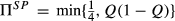
Our theoretical analyses establish an equilibrium pricing structure and show how the key model primitives affect regular and markdown prices, as well as sales and revenues. We characterize the conditions under which one of two fundamentally different pricing strategies is optimal. If the fraction of strategic consumers in the population is above a certain threshold, the retailer targets both (TB) myopic and strategic consumers in the early season, which requires low markdowns to sell to both consumer types in the early season. In contrast, if the fraction of strategic consumers is below the threshold, the retailer targets only myopic (TM) consumers in the early season, which requires high markdowns to divert all strategic consumer demand to the late season. Under the TM strategy the retailer forgoes the opportunity to inter‐temporally price‐discriminate strategic consumers to extract more revenue from myopic consumers. Surprisingly, the threshold (between TB and TM) tends to be quite high, providing fairly broad conditions under which it is optimal to purposefully forgo all demand from strategic consumers in the early season, with the possible implication that most revenue is obtained in the late season.

Our model refines many models already in the literature (see section 2) toward some empirical regularities. On the consumer side, our model is among a few that capture the important and well‐established phenomenon that some consumers are strategic while others are myopic (Li et al. 2014, Mak et al. 2014). On the retailer side, the qualitative predictions from our model align with the pricing and sales patterns that seem to characterize many retail environments. Indeed, Kaufmann et al. ( 1994) suggest that in the 1990s, 60–70% of merchandize was sold with some markdown, and Kapner ( 2013) notes that in 2012, a major U.S. retailer “was selling fewer than one out of every 500 items at full price.” This evidence matches well with our prediction under the TM policy, which calls to set large markdowns and sell only a few items in the early season.

How Do People Price?

We test our theoretical predictions in a laboratory experiment. We find that subjects generally benefit from the opportunity to price dynamically, and fare better than the static pricing benchmark of a retailer committing to a single price in both seasons. In fact, in the baseline conditions without strategic consumers, subjects price optimally after gaining experience with the task. In the conditions with a moderate fraction of strategic consumers (where a TM policy is optimal), and again after significant learning, subjects offer steep markdowns and move significant revenue to the late season, as predicted. However, in such conditions, subjects price below equilibrium in the early season, which leads to larger than equilibrium sales and often above‐equilibrium revenues in the early season, but limits the ability to generate revenue at markdowns. We term this behavior “myopia,” as it is consistent with a general notion of nearsightedness and undervaluing the future in favor of the present.¹ We find some evidence for the hypothesis that the observed underpricing pattern persists in conditions with a moderate fraction of strategic consumers because the optimal pricing structure requires a shift towards a regime where most revenue is obtained in the late season, which may be counter‐intuitive so as to inhibit efficient learning.

Our study also sheds light on the effect of inventory scarcity on pricing decisions. As one would expect, our model predicts that prices are non‐increasing in inventory. Indeed, we observe strong evidence that prices are lower in treatments with truly limited inventory (when it was optimal to sell all units) than in those with unlimited inventory (when it was impossible to sell all units). However, we also observe a weaker effect that subjects underprice the most when inventory limit was perceived rather than actual – i.e., when it was possible, but not optimal, to sell all units. This maps well onto existing studies of the impact of perceived scarcity on decision making (e.g., Mullainathan and Shafir 2013).

Literature Review

Our study is related to two bodies of literature: modeling and behavioural.

Modeling Literature

We investigate pricing decisions in a no‐replenishment two‐period capacitated monopoly setting with a mix of myopic and strategic consumers and heterogeneous valuations that are constant over time. This setting, to the best of our knowledge, has not been comprehensively addressed in the significant body of modeling research on strategic consumers (see Table D1 in Appendix D).² For example, many studies assume that all consumers are strategic (e.g., Aviv and Pazgal 2008, Besanko and Winston 1990, Coase 1972, Dasu and Tong 2010, Liu and van Ryzin 2008, Stokey 1979). In contrast, we model a mix of myopic and strategic consumers, which is an assumption that is supported empirically.

Our study also departs from the previous work in terms of our treatment of consumer valuations. Cachon and Swinney ( 2009) assumed that myopic consumers who did not purchase during the main selling season are replaced with bargain‐hunting consumers whose valuations are independent of the myopics’ initial valuations. Levin et al. ( 2009) made a similar assumption that consumers’ valuations during markdowns are redrawn randomly. Su ( 2007), Lai et al. ( 2010), and Ovchinnikov and Milner ( 2012) restricted valuations to only take a few values (e.g., high and low), which again does not quite capture the shopping situation we study. Gallego et al. ( 2008), Zhang and Cooper ( 2008), and Mersereau and Zhang ( 2012) considered the case with a mixture of myopic and strategic consumers, and with finite inventory, but under price commitment – i.e., a situation when future prices are pre‐announced and are known to consumers. In contrast, we consider a situation in which firms can adjust prices dynamically in response to early season sales, as they do in practice.

Behavioral Literature

In contrast to the relatively mature modeling literature, behavioral studies of strategic consumer behavior and its implications for dynamic pricing and revenue management are relatively scarce. First and foremost, a distinction must be made between studies of buyer/consumer behaviors, which seek to understand if consumers are indeed strategic and how strategic they are, and studies of sellers’ behaviors, to which our study belongs.

Regarding buyers’ behavior, Li et al. ( 2014), based on data from the air‐travel industry, found that 5–20% of buyers could be classified as strategic. Mak et al. ( 2014) found that, in a given round of their experiment, 17–41% of buyers bought myopically, and 6–13% waited irrationally (Table 2 in their paper). Osadchiy and Bendoly ( 2010) also find that while many are strategic, some subjects in their experiments are consistently buying myopically. The main implication of this literature for our study is that it provides empirical support for our model with a mixture of both strategic and myopic consumers.

Regarding sellers’ behavior, in the operations management literature, Bearden et al. ( 2008) arguably performed the first laboratory experiment within the context of dynamic pricing and revenue management. In their setting, monopolistic sellers (played by human subjects) decide on accepting or rejecting bids from computer‐generated myopic customers. Bendoly ( 2011) uses a similar setting to study behaviors when subjects manage multiple sources of revenue, while Bendoly ( 2013) studies the impact of feedback provided. The key pricing observation from these studies is “a clear pattern of being too demanding when holding higher levels of inventory and insufficiently demanding when holding lower levels” (Bearden et al. 2008). Since levels of inventory are negatively correlated with time, their pattern thus implied that subjects overpriced early in the selling horizon, but underpriced toward the end. Kocabiyikoglu et al. ( 2015) study the behavioral similarity between setting protection limits in a two‐class revenue management system and deciding on order quantities in a newsvendor problem (these are analytically equivalent). They observe that subjects overprotect inventory, which is similar to overpricing early in the selling horizon. Neither of these studies, however, consider strategic consumers. Mak et al. ( 2015) consider retailers’ pricing with strategic consumers in a unique setting where both strategic buyers and sellers are played by human subjects. Our work (in which buyers are automated, but a mixture is considered) complements their study.

In the economics literature, in a laboratory study of dynamic pricing in a durable‐goods monopoly with a single human seller and 1–5 human buyers, Reynolds ( 2000) observe “substantial demand withholding,” implying that (some of) the buyers were indeed strategic. He observes that sellers consistently overprice in the contingent pricing case. Cason and Mago ( 2013) presents the results of a laboratory study in which two (human) sellers compete to sell to a single potentially patient (human) buyer. They find that underpricing occurs in a single‐round game, but overpricing is common the multiple‐rounds game that resembles our early/late season setting. Mak et al. ( 2012) present and empirically test a model of dynamic pricing when sellers place alternating offers to sell a unit of the product to a single buyer. They observe that prices are generally consistent with the model predictions if the buyer is myopic, but significantly above optimal if the buyer is strategic.

Theoretical Model

Consider a market with a single retailer who is endowed with Q units of a good to sell over a horizon that consists of two periods (seasons): early season and late season. The market consists of N consumers whose individual valuations for the good, v, are uniformly distributed over [0, b]. This distribution is common knowledge, but each individual consumer's valuation is not known to the retailer. To simplify the exposition, we normalize the market size, N = 1; similarly, we assume the upper bound on consumers’ valuations, b = 1 (later, in the behavioral experiment, we assign different values to N and b). We consider contingent pricing: in the early season, the retailer decides on its early‐season price, and then in the late season, the retailer selects its late‐season price.

A fundamental feature of our problem is that consumers can be either myopic or strategic.³ A myopic consumer purchases the good as soon as the posted price is below her valuation. In contrast, a strategic consumer optimally times her purchase in order to maximize the expected surplus. Given the early‐season price she sees,

p_{E}

, and the late‐season price she expects to see if she waits,

p_{L}

, a strategic consumer will purchase in the early season if her immediate early‐season surplus,

v - p_{E},

exceeds her discounted expected surplus from the late season,

δ (v - p_{L}),

where δ is a discounting factor that we assume to be identical for all strategic consumers (Aviv and Pazgal 2008, Besanko and Winston 1990); otherwise, she will wait for the late season. This gives rise to a threshold valuation,

V \equiv m i n {\frac{p_{E} - δ p_{L}}{1 - δ}, 1},

such that all strategic consumers with v < V wait for the late season. We assume that a fraction α of the consumers behave strategically whereas the fraction of 1 − α consumers behave myopically (see Su 2007, and Cachon and Swinney 2009, for a similar market segmentation).

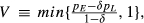
Table 1 presents the demand and sales for each consumer segment, given prices

p_{E}

p_{L}

, and the resultant threshold valuation V. The retailer's total revenue is:

Π = π_{E} + π_{L} \equiv p_{E} S_{E} + p_{L} S_{L} .

Table 1
Demand from and Sales to Each Consumer Segment By Season

Early season Late season

Myopic demand $(1 - α) (1 - p_{E})$
$(1 - α) p_{E} (1 - \frac{p_{L}}{p_{E}})$

Strategic demand α(1 − V)
$α V (1 - \frac{p_{L}}{V})$

Total demand
$D_{E} = \sum$
of above
$D_{L} = \sum$
of above

Total sales
$S_{E} = min {Q, D_{E}}$

$S_{L} = min {Q - D_{E}, D_{L}}$

	Early season	Late season
Myopic demand	$(1 - α) (1 - p_{E})$	$(1 - α) p_{E} (1 - \frac{p_{L}}{p_{E}})$
Strategic demand	α(1 − V)	$α V (1 - \frac{p_{L}}{V})$
Total demand	$D_{E} = \sum$ of above	$D_{L} = \sum$ of above
Total sales	$S_{E} = min {Q, D_{E}}$	$S_{L} = min {Q - D_{E}, D_{L}}$

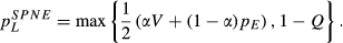
The model is solved backwards to yield the subgame perfect Nash equilibrium (SPNE). Given

p_{E}

and V, it is easy to verify that the optimal subgame perfect late‐season price equals:

p_{L}^{S P N E} = max \{\frac{1}{2} (α V + (1 - α) p_{E}), 1 - Q\} .

Consumers’ Expectations

While a myopic consumer simply buys in the early season when

v > p_{E},

a strategic consumer needs to form an expectation about the late‐season price and availability of the good. To model such an expectation formation process, we make the following assumption that links the early‐season price to the late‐season price:

Assumption 1 Conditionally Optimal Late‐Season Price

Strategic consumers assume that given the observed early‐season prices, the retailers will price optimally in the late season.

Assumption 1 is a revelation of rational expectations (Cachon and Swinney 2009, Su 2007) in the sense that once the retailer moves to the late season, it will maximize the late‐season revenue given the demand it encounters. It is not difficult to show that this implies that the retailer has no incentive to ration inventory, which contrasts with the results of Liu and van Ryzin ( 2008), Zhang and Cooper ( 2008), and Mersereau and Zhang ( 2012), who show that rationing may be optimal. This is because these studies consider price commitments, while we consider contingent pricing.

Let

{\hat{p}}_{L} (p_{E})

denote the price that strategic consumers expect to see in the late season upon observing price

p_{E}

. Substituting the expression from equation (2) into the definition of the threshold valuation V, we simultaneously solve for V and

p_{L}

, and obtain the following result (the proof of this specific result follows from the above discussion and is thus omitted; otherwise, all proofs are in Appendix A):

Lemma 1

Seeing

p_{E}

in the early season, a strategic consumer expects price

{\hat{p}}_{L} (p_{E})

in the late season. Consumers with valuations with

v > V (p_{E})

will buy early, while those with

v \leq V (p_{E})

will wait, where

\begin{matrix} V (p_{E}) = min \{1, max \{\frac{p_{E} (2 - δ + δ α)}{2 - 2 δ + δ α}, \frac{p_{E} - δ (1 - Q)}{(1 - δ)}\}\}, \\ {\hat{p}}_{L} (p_{E}) = max \{1 - Q, min \{\frac{α + p_{E} (1 - α)}{2}, \frac{p_{E} (δ α - δ + 1)}{2 - 2 δ + δ α}\}\} . \end{matrix}

Note that whenever V = 1, no strategic consumers are buying in the early season. We refer to such cases as Target Myopic (TM), which can be either capacitated (cTM, when all inventory is sold) or uncapacitated, (uTM, when some inventory remains unsold). In reverse cases, with V < 1, both myopic and strategic consumers are purchasing in the early season. We refer to these cases as Target Both (TB), and similarly, they can be capacitated (cTB) or uncapacitated (uTB). Technically, there also is a possibility to sell‐out early, SOE, in which case there is no late season. It is easy to show that SOE is never optimal; hence, we omit this possibility from further consideration.

Model Predictions

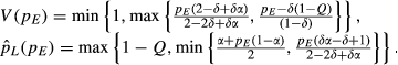
Having solved the late‐season subgame and characterized the behavior of the strategic consumers, we substitute the late‐season price and the corresponding threshold valuation equation (3) into equation (1) and solve for the SPNE early‐season prices.

Proposition 1

There exist thresholds for α and Q such that one of the four pricing policies emerges in equilibrium (uTB, uTM, cTB, or cTM) with prices and profits as follows: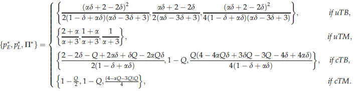

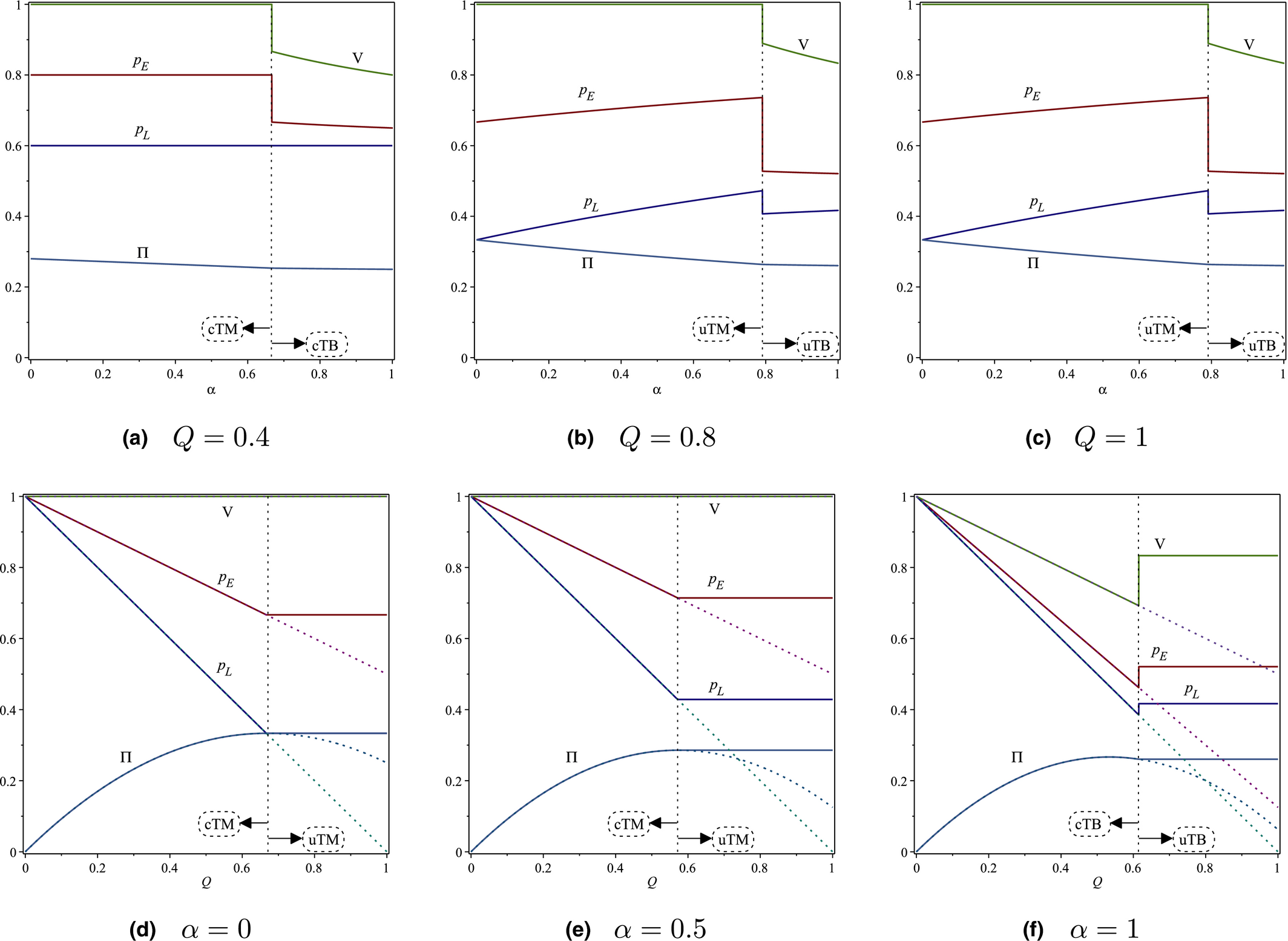
{p_{E}^{*}, p_{L}^{*}, Π^{*}} = \{\begin{matrix} \{\frac{{(α δ + 2 - 2 δ)}^{2}}{2 (1 - δ + α δ) (α δ - 3 δ + 3)}, \frac{α δ + 2 - 2 δ}{2 (α δ - 3 δ + 3)}, \frac{{(α δ + 2 - 2 δ)}^{2}}{4 (1 - δ + α δ) (α δ - 3 δ + 3)}\}, & i f u T B, \\ \{\frac{2 + α}{α + 3}, \frac{1 + α}{α + 3}, \frac{1}{α + 3}\}, & i f u T M, \\ \{\frac{2 - 2 δ - Q + 2 α δ + δ Q - 2 α Q δ}{2 (1 - δ + α δ)}, 1 - Q, \frac{Q (4 - 4 α Q δ + 3 δ Q - 3 Q - 4 δ + 4 α δ)}{4 (1 - δ + α δ)}\}, & i f c T B, \\ \{1 - \frac{Q}{2}, 1 - Q, \frac{(4 - α Q - 3 Q) Q}{4}\}, & i f c T M . \end{matrix}

The TB/TM structure of the equilibrium pricing policy makes intuitive business sense. When sufficiently many consumers are myopic (“low” α), it is optimal to charge a high price in the early season, extracting revenue from myopic consumers and diverting all strategic consumers to the late season. That is, the firm foregoes the opportunity to intertemporarily price‐discriminate strategic consumers in order to better price‐discriminate myopic consumers – a TM policy. However, when most consumers are strategic (“high” α), foregoing such an opportunity is not profitable; hence, the firm charges a lower price in the early season, selling to both strategic and myopic consumers – a TB policy. Note that “low” and “high” here pertain to the thresholds defined in the proof of the proposition; for example, when Q ∈ {0.8, 1}, as can be observed from panels (b) and (c) of Figure 1, even α ≈ 0.7 may still be “low.” That is, the TM policy is optimal for a wide range of parameters; importantly, including the fractions of strategic consumers that were documented empirically.

Figure 1

Optimal Prices, Threshold Valuation, and Profit as a Function of α and Q for δ = 0.75

Impact of Strategic Consumers

Proposition 2

Under all pricing policies, the revenue is decreasing in α. The early‐season price decreases in α under TB policies (cTB and uTB), increases under uTM, and does not change in α under cTM. The late‐season price increases in the uncapacitated policies (uTM and uTB) and does not change in α in the capacitated policies (cTM and cTB).

The proposition shows that equilibrium revenues are decreasing, and the late‐season price is non‐decreasing, in the fraction of strategic consumers. However, the early‐season price is non‐increasing under TB and non‐decreasing under TM. Intuitively, under TB, as α increases, the retailer tries inducing strategic consumers to purchase in the early season and thus he decreases the early‐season price. But under TM the retailer seeks to divert all strategic consumers to the late season, and thus he raises the early‐season price. Late‐season prices increase because the more strategic consumers there are, the larger late season demand is. Combining both effects, an increase in α leads to a decrease in revenues, as strategic consumers intensify inter‐temporal competition. See panels (a–c) of Figure 1 for an illustration. Evidently, in the capacitated settings (panel (a)), the late‐season price does not change in α since this price already clears the market. Further, under cTM, the early‐season price does not change in α since all strategic consumers already wait for the late season and hence no price adjustment is required.

The next proposition characterizes the distribution of revenue across seasons.

Proposition 3

Under all pricing policies, the proportion of revenue generated in the early season,

π_{E} / Π,

decreases in α. Further, there exists a threshold,

\bar{α},

such that if

α \geq \bar{α}

then

π_{E} / Π \leq 0.5,

where

{\bar{α}}_{c T B} = 0,

{\bar{α}}_{c T M} = Q / (4 - 3 Q),

{\bar{α}}_{u T B} = (1 - δ) / δ,

and

{\bar{α}}_{u T M} = (\sqrt{17} - 3) / 4 .

That is, with sufficiently many strategic consumers, the retailer obtains most of its revenue in the late season. This is again related to the fact that it may be optimal to shift all strategic consumers’ demand to the late season, while serving only high‐valuation myopic consumers in the early season, selling them only a few units of inventory, but at high prices. This counterintuitive finding will play an important role in the experimental part of our study.

Impact of Inventory

When inventory is large, the policy is uncapacitated; it is more profitable for the retailer to leave some units unsold because selling them requires charging an excessively low price, which would incentivize strategic waiting. Conversely, when inventory is small, the retailer can profitably sell all the inventory; hence, the policy becomes capacitated.

Proposition 4

Under capacitated policies, both the early‐ and late‐season prices decrease in Q, whereas under uncapacitated policies, the prices are independent of Q.

That is, both early‐ and late‐season prices decrease in the available inventory when the retailer follows a capacitated pricing policy: with more inventory, the retailer sets a lower price in the late season (to sell out); this induces strategic waiting and to counter it, the retailer also sets a lower price in the early season. When the retailer follows an uncapacitated pricing policy, the prices are independent of the inventory, as the inventory exceeds the amount required to implement the optimal pricing. See panels (d–f) of Figure 1.⁴

Behavioral Experiment

Does our model accurately describe how people price in the presence of strategic consumers? To answer this question we designed an experiment to test the equilibrium predictions from our model under controlled laboratory conditions.

Design and Implementation

Decision Task

The subjects in our experiment acted as pricing managers, facing a population of N = 100 consumers automated as per Section 3.1. The first consumer has a valuation of 1, the second has a valuation of 2, etc. While this is, technically speaking, different from the continuum of consumers that our model assumes, the discretization is fine enough to represent a continuum well (Mago and Dechenaux 2009). Note that this implementation eliminates any uncertainty about the valuation distribution, which is consistent with our model premises; it facilitates learning, and is similar to the “no‐replacement” procedure used in Mak et al. ( 2015) to assign (human) buyers valuations from a fixed set of uniformly distributed values. As discussed in the literature review section, the decision to automate consumers represents a strategic choice in our experimental design – it allows us to isolate the impact of strategic consumer behavior, as well as to capture a realistic retail‐like setting where there are many more buyers than sellers.

Predictions and Design

To test the key predictions of our model, we vary strategic behavior (α = {0, 0.5}) and available inventory (Q = {40, 80,100}), resulting in six treatments that we implement in a between‐subject design.

Our first model prediction concerns the effect of strategic consumers. Our design includes treatments without strategic consumers (α = 0) as an experimental baseline. Our focus is on pricing behavior in the presence of myopic and strategic consumers, which aligns with the conditions in many markets. To this end, our design includes treatments with α = 0.5, for which Proposition 2 predicts that prices go up, relative to environments without strategic consumers. While this prediction is eminently sensible, our analysis reveals fairly broad conditions under which all strategic customers are priced out of the early season with a possible consequence that the firm earns most of its revenue in the late season (Proposition 3). The application of this policy requires consequential thinking, a principle that most decision makers fail to apply even in fairly simple settings (Shafir and Tversky 1992). Furthermore, diverting most revenues to the late season runs counter to the intuitive strategy of using the late season primarily to sell to a few more customers with a lower willingness‐to‐pay. Our experiments are designed to test whether human decision makers set their prices dynamically in ways consistent with this prediction, and if not, then why.

Our second model prediction concerns the effect of inventory scarcity, and our design includes three levels of available inventory. The case of Q = 100 serves as an uncapacitated baseline for which inventory scarcity is a non‐issue (as Q = N = 100). While scarcity never drives prices down, Proposition 4 distinguishes between scarcity that leads to price increases in a capacitated policy (Q = 40 in our design), and scarcity that does not affect prices in an uncapacitated policy (Q = 80 in our design). In other words, our choices for Q allow us to investigate the difference between actual scarcity (Q = 40) and perceived scarcity (Q = 80). Of course, the precise boundary between capacitated and uncapacitated policies is a technical condition that is not likely to be immediately obvious to human decision makers. Mullainathan and Shafir ( 2013, p. 11) argue that the “feeling of scarcity is distinct from physical reality,” suggesting that scarcity may affect observed prices even in an uncapacitated regime (Q = 80), where it should not. Our experiment is designed to study that as well.

Discount Factor

Across all treatments, we keep consumers’ discounting factor at δ = 0.75. Our choice of discounting factor is consistent with the experimental evidence for time discounting and the length of the selling season observed in practice. Most retailers have two markdowns per year: Christmas sales and summer sales. Thus, “a period” in the language of our study is 6 months, of which for some 4–5 months the retailer holds regular prices (“early season”), and during the 1–2 months of sale, the prices are marked down (“late season”).” By our model assumption, all consumers are present at the beginning of the period; thus, the time delay between the “buy” and “wait” options is approximately 4–5 months. Using experimental data for exponential discount function exp [−rt] with t = 1 month Baucells et al. ( 2013) estimated modal r = 6.6% for prospects of approximately 50–100 EUR (a reasonable value in the retail context we consider). Hence, a discount factor of 0.75 = exp [−0.066t] corresponds to t = 4.36 months, which matches the duration of the delay in practice.

Task Interface

We coded the experimental interface in zTree (Fischbacher 2007) and provide sample screenshots in Appendix B. Each round of the experiment started with an early‐season screen, which contained a visual 10 × 10 array of grey dots depicting the N = 100 consumers, a clearly visible number of consumers who visit the retailer's store, the history of the experiment so far, and one empty box to enter the early‐season price. Upon submitting the price, the system determined which consumers purchased and which waited, as per sub section 3.1, and then transitioned to the late‐season screen. The late‐season screen contained both visual and numerical information about the early‐season prices and sales, as well as information about revenues; we used colored dots to represent those consumers who already purchased. It also contained both visual and numerical information about the number of consumers who visited the retailer in the late season, as well as one empty box to enter the late season price. Generally, threshold valuations, and therefore sales, can be fractional; thus, to avoid confusion, the interface rounded the numbers of consumers to integers. Finally, after submitting the late‐season price, the subject saw the end‐of‐the‐round screen, which summarized the results of the round, again, both visually and numerically.

Subjects and Payments

Participants were recruited from an experimental subject pool at a major North American university. Upon showing up to a lab, they were given the instructions to read (see Appendix C for a sample), and they then watched a short presentation with the snapshots of the experimental interface. The presentation emphasized the two‐period structure, decisions, market composition (specifically, that being strategic is independent of valuation), revenue calculations, and payments. Subjects then proceeded with the experiment: first, they played 2 rounds for demonstration purposes, and then they played 30 more rounds from which the data were collected. Each subject was compensated in proportion to the total revenue in those 30 rounds, plus a $5 participation fee; compensation varied from $5 to $30 with an average of $19.24. Participants were paid in private at the end of the session; cash was the only incentive offered.

Preliminaries

For each subject i, our data comprise observations for periods t = 1 … 32, both for the early (E) and the late⁵ (L) season. We use the “tilde" symbol to denote the observed pricing decision of subject i, (e.g.,

{\tilde{p}}_{E, i, t}

), as well as the resulting revenue (e.g.,

{\tilde{π}}_{E, i, t}

). We omit subscript i to denote averages over subjects, e.g.,

{\tilde{p}}_{E, t} .

Similarly, we omit t to average over periods, e.g.,

{\tilde{p}}_{E, i} .

To assess observed decisions relative to theoretical predictions, let the “asterisk" symbol denote the optimal price and revenue (e.g.,

p_{E}^{*},

π_{E}^{*}

), with the understanding that these benchmarks are treatment‐specific. Recall also that the “hat" symbol (e.g.,

{\hat{p}}_{L}

) refers to the conditionally optimal late‐season quantities.

Figures 2 and 3 display subject‐averaged revenues and prices over time. Without a formal analysis, we can observe noticeable learning in the early periods of the experiment. Generally, prices and revenues approach theoretically predicted levels. We address the issue of learning in more depth later in sub section 4.4. For now, in order to give theory its best shot, we are interested in subjects’ choices after they have gained experience with the pricing task. To this end, we compare our data with the model benchmarks for the second half of the experiment, t = 17 … 32. Note that the cutoff in the middle (at t = 16) is natural, but ultimately as arbitrary as any other cutoff. We tested cutoffs at t = 13 … 22 and the qualitative findings are identical. Table 2 presents the results along with some relevant statistical tests. Unless noted otherwise, the reported statistical tests are two‐sided and use subject‐level averages as the unit of analysis; standard errors are in parentheses.

Figure 2

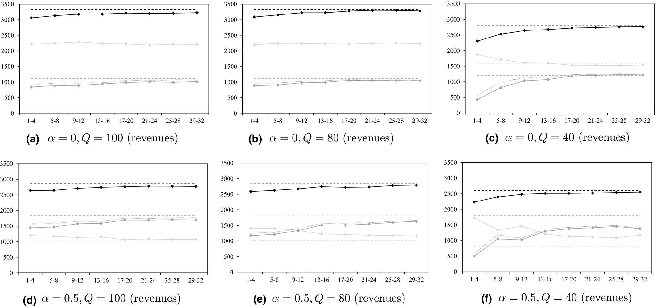
Revenues (π) By Treatment (Total: — data −−− theory, early: — data −−− theory, late: − data −−− theory, ‐‐‐ cond. optimal)

Figure 3

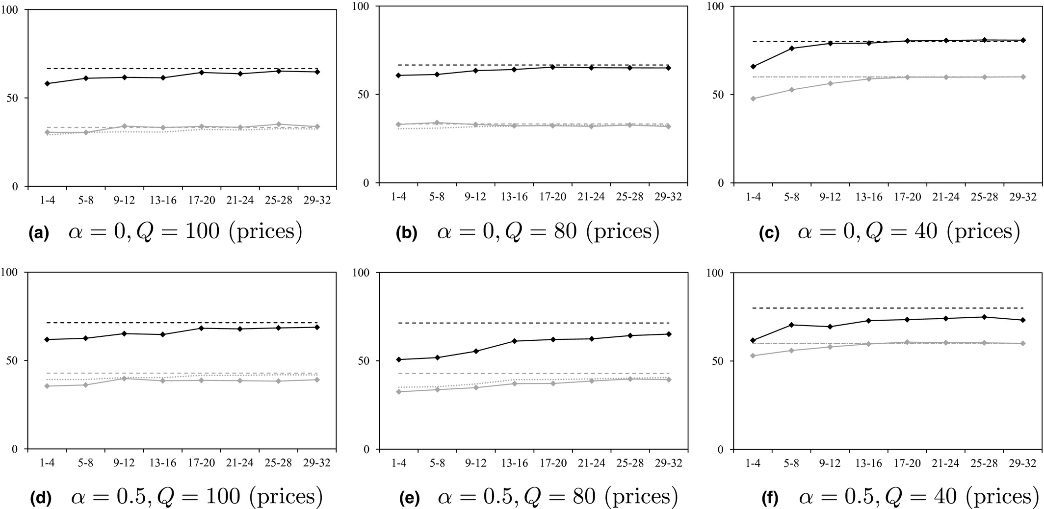
Prices (p) By Treatment (early: −−−− data — theory, late: −−− data −− theory, −−− cond. optimal)

Table 2

Revenues and Prices, t ≥ 17

$α$	Q	N	Revenue					Early price			Late price
$α$	Q	N	$Π^{S P}$		Observations		Π *	Observations		p_E *	Observations		p_L *		${\hat{p}}_{L}$
0	100	14	2500	< **	$\underset{(80.89)}{3211}$	−	3333	$\underset{(1.46)}{64.52}$	−	66.66	$\underset{(2.04)}{34.08}$	−	33.33	−	$\underset{(0.73)}{32.26}$
0.5	100	23	2500	< **	$\underset{(23.46)}{2774}$	< **	2857	$\underset{(1.75)}{68.36}$	−	71.42	$\underset{(1.43)}{38.71}$	< **	42.85	−	$\underset{(0.59)}{41.74}$
0	80	22	2500	< **	$\underset{(16.47)}{3290}$	< *	3333	$\underset{(0.73)}{65.15}$	−	66.66	$\underset{(0.81)}{32.18}$	−	33.33	−	$\underset{(0.36)}{32.18}$
0.5	80	23	2500	< **	$\underset{(21.04)}{2757}$	< **	2857	$\underset{(2.21)}{63.49}$	< **	71.42	$\underset{(1.17)}{38.61}$	< **	42.85	−	$\underset{(0.93)}{39.87}$
0	40	26	2400	< **	$\underset{(12.03)}{2749}$	< **	2800	$\underset{(0.57)}{80.67}$	−	80	$\underset{(0.55)}{59.31}$	−	60	−	$\underset{(0)}{60}$
0.5	40	23	2400	< **	$\underset{(14.90)}{2533}$	< **	2600	$\underset{(1.48)}{73.94}$	< **	80	$\underset{(2.63)}{57.43}$	−	60	−	$\underset{(0)}{60}$

Double‐sided t‐tests reported where − means insignificant, otherwise **p = 0.01, *p = 0.05.

Our experiment automates strategic consumers according to Assumption 1. That is, given subjects’ early season prices

{\tilde{p}}_{E}

(however suboptimal those may be) in the late season, strategic consumers expect to see conditionally optimal prices

{\hat{p}}_{L} ({\tilde{p}}_{E}) .

The right panel in Table 2 confirms that the observed prices are indeed statistically not different from conditionally optimal ones in all six treatments of our experiment. This provides an important consistency check for our experiment, and allows us to move forward to analyze its results.

Main Results

We first test the comparative statics regarding the impact of strategic consumers and inventory scarcity on prices and revenues.

Impact of Strategic Consumers (Proposition 2)

For the treatments covered in our experimental design (TM pricing policies), Proposition 2 predicts that the total revenues do not increase, and that both early‐ and late‐season prices do not decrease in the fraction of strategic consumers. We find that total revenue is indeed smaller at α = 0.5 than at α = 0, based on pairwise comparisons at each level of Q. However, early‐season prices do not increase in α when they are predicted to change for Q = 100 and Q = 80, and even decrease when they are predicted not to change in α for Q = 40. Similarly, late‐season prices increase in α only for Q = 80. In other words, we find that prices are not sufficiently sensitive to the fraction of strategic consumers.

Impact of Inventory Scarcity (Proposition 4)

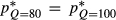
Proposition 4 predicts that both early‐ and late‐season prices decrease in Q, in capacitated regimes. Recall that the parameters of our experiment were selected so that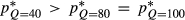

p_{Q = 40}^{*} > p_{Q = 80}^{*} = p_{Q = 100}^{*}

, for both levels of α. Our data mostly aligns with this prediction. In the absence of strategic consumers (α = 0), prices in Q = 40 are higher than in Q = 100, both in the early season (80.67 vs. 64.52, p < 0.01) as well as in the late season (59.31 vs. 34.08, p < 0.01). Similarly, in the presence of strategic consumers (α = 0.5), prices in Q = 40 are higher both in the early season (73.94 vs. 68.36, p < 0.01) as well as in the late season (57.43 vs. 38.71, p < 0.01). In contrast to the effect of “actual” scarcity, the theory predicts no impact of “perceived” scarcity,

p_{Q = 80}^{*} = p_{Q = 100}^{*}

. In the absence of strategic consumers (α = 0), the average early‐season prices indeed do not differ between Q = 100 and Q = 80 (65.15 vs. 64.52, p = 0.67), and neither do late‐season prices (32.18 vs. 34.08, p = 0.40). With strategic consumers (α = 0.5), the early‐season prices with Q = 80 units are lower than with Q = 100 (63.49 vs. 68.36, p = 0.09), but the effect is only weakly significant. Overall, regarding the impact of scarcity on prices, the observed pricing behavior is correct in a qualitative sense.

Data Vs. Theory (Proposition 1)

We next compare pricing behavior with the equilibrium benchmarks from Proposition 1. Without strategic consumers (α = 0), both early‐ and late‐season prices are statistically indistinguishable from theory predictions, at all levels of Q (Table 2). In contrast, in the presence of strategic consumers (α = 0.5), we observe that subjects underprice in the early season for Q = 80 (63.49 vs. 71.42, p < 0.01) and Q = 40 (73.94 vs. 80, p < 0.01). For Q = 100, they also underprice, but only insignificantly so (68.36 vs. 71.42, p = 0.09 ). Although late‐season prices also tend to be lower than the equilibrium benchmark,

p_{L}^{*}

, it is important to note that the latter is not conditionally optimal. Given the early season underpricing we observe, the retailer maximizes revenue in the late season by charging a conditionally optimal late‐season price,

{\hat{p}}_{L}

. In all conditions, observed prices are not statistically different from

{\hat{p}}_{L}

Revenue Impact

The observed early‐season underpricing in the presence of strategic consumers is statistically and economically significant. The magnitude of the total revenue loss (compared to

Π^{*}

) may seem small, e.g., in the (Q = 80, α = 0.5) treatment, the average loss is 2857−2757 = 100 or about 3% of the revenue. However, this number should be put into perspective of the revenue opportunity: the incremental revenue that the firm can make on top of the revenue it generates with static pricing. Under static pricing, denoted by SP, strategic consumers expect to encounter the same prices in the early and late seasons, thus

{p_{E}^{S P}, p_{L}^{S P}} = {max {\frac{1}{2}, 1 - Q}, max {\frac{1}{2}, 1 - Q}},

and

Π^{S P} = min {\frac{1}{4}, Q (1 - Q)}

. Note that the entire revenue is obtained in the early season. In this example the static revenue

Π^{S P} = 2500

, and

(\frac{2757 - 2500}{2857 - 2500}) \approx 0.7,

i.e., subjects lost nearly 30% of the revenue opportunity.

Revenue Distribution (Proposition 3)

Besides the obvious loss in total revenue, such underpricing with α = 0.5 affects the distribution of sales and revenues across seasons (early vs. late).

Subjects sold more than optimal in the early season in the Q = 40 (16.11 vs. 10, p < 0.01), the Q = 80 (20.54 vs. 14, p < 0.01), and the Q = 100 (16.78 vs. 14.29, p = 0.03) treatments. Combining the price and sales effects, subjects generally obtained higher than optimal early‐season revenue for Q = 40 (1127 vs. 800, p < 0.01) and Q = 80 (1184 vs. 1020, p < 0.01), although the effect is not significant for Q = 100 (1074 vs. 1020, p = 0.13). Subjects also obtained lower than optimal late‐season revenues: for Q = 40 (1406 vs. 1800, p < 0.01), for Q = 80 (1572.5 vs. 1836, p < 0.01), for Q = 100 (1699 vs. 1836, p = 0.01). Further, the conditionally optimal late season revenue was also below optimal: for Q = 40 (1438 vs. 1800, p < 0.01), for Q = 80 (1616 vs. 1836, p < 0.01), and for Q = 100 (1755 vs. 1836, p = 0.08). By underpricing in the early season, subjects have discouraged waiting and increased their immediate revenue; however, by doing so, they not only reduced the potential late‐season demand, but also limited the late‐season price (since the conditionally optimal price is lower), ultimately diminishing the total revenue over the two seasons.

Why Myopia?

In the presence of strategic consumers (α = 0.5), our data reveals a pattern that we refer to as myopia – the tendency to underprice, oversell, and obtain a larger than optimal revenue in the early season at the expense of the possibility of obtaining revenue later.

To understand why this might be happening, note that the “opening" (initial) prices made in the first paid round of the experiment (i.e., decisions before subjects gained significant experience, t = 3) are not sensitive to α. Table 3 presents the opening prices and suggests that subjects do not immediately understand what strategic consumers imply for the optimal pricing structure. When theory predicts higher early‐season prices with (α = 0.5) than without (α = 0) strategic consumers, the data either shows no difference (Q = 100: 57.78 vs. 63.04, p = 0.23; Q = 0.4: 66.77 vs. 64.09, p = 0.41) or a lower price for α = 0.5 (Q = 80: 50.83 vs. 57.45, p = 0.05). Importantly, subjects initially underprice in all six treatments (p < 0.02).

Table 3

Opening Early‐Season Prices Per Treatment, Averaged By Subject

α	Q = 100		Q = 80		Q = 40
0	57.78	−	57.45	<^*	66.77
	\|		∨^*		\|
0.5	63.04	>^*	50.83	<^*	64.09

− means insignificant, **p = 0.01, *p = 0.05.

That is, subjects started the experiment by exhibiting myopia in all treatments, but in treatments without strategic consumers, α = 0, they were able to learn how to price optimally, while in those with strategic consumers, α = 0.5, they did not. This therefore suggests that the key to understanding the persistence of myopia is in studying how the presence of strategic consumers affected subjects’ learning. To be clear, subjects learned in all treatments, and this is hardly surprising: our experiment features deterministic feedback, so subjects explore prices and stick to those that lead to higher revenues. The surprising finding is that learning helps subjects overcome their initial pricing bias with α = 0, while learning remains insufficient with α = 0.5, with myopia as the principal implication.

We posit that subjects exhibit insufficient learning for α = 0.5 because of what the optimal policy implies with regard to the distribution of sales and revenues across selling seasons. Intuitively, one would expect that firms should make most of their revenue in the early (main) selling season, when they have a lot of inventory and high prices, and only sell few of the remaining items (and at lower prices) during the late (markdown) season. Without strategic consumers (α = 0), this is indeed optimal: the firm is predicted to make most of its revenue in the early season (

π_{E}^{*} > π_{L}^{*}

), and we observe just that. While subjects initially underprice (in t = 1), they quickly learn how to price optimally, and they earn more revenue in the early season than in the late season,

{\tilde{π}}_{E, t} > {\tilde{π}}_{L, t}

In contrast, with strategic consumers (α = 0.5), our theoretical analysis predicts that the firm prices all strategic consumers out of the early season, diverting most revenue to the late season (

π_{E}^{*} < π_{L}^{*}

). While they initially (t = 3) underprice and “over‐earn” in the early season, subjects learn to shift revenues to the late season. However, in contrast to α = 0, the learning process requires them to cross (when Q = 40, 80), or cross further (when Q = 100), into a pricing regime with a counterintuitive distribution of revenues with

{\tilde{π}}_{E, t} < {\tilde{π}}_{L, t}

; see Figure 2d–f. This, we believe, renders their learning slow and ultimately incomplete.

To test this hypothesis, let

x_{i, t}

be an indicator variable for crossing in period t;

x_{i, t} = 1

{\tilde{π}}_{E, t} < {\tilde{π}}_{L, t}

, and

x_{i, t} = 0

otherwise. Further, let

Δ_{i, t}^{p} = {\tilde{p}}_{E, i, t} - {\tilde{p}}_{E, i, t - 1}

measure the extent to which subjects explore possible prices. We find a significant difference between the conditional means,

Δ_{i, t}^{p} |_{x_{i, t - 1} = 1} = - 0.18

and

Δ_{i, t}^{p} |_{x_{i, t - 1} = 0} = 0.76

(p < 0.01, two‐sample unequal variances t‐test), which suggests that learning slows following a period with crossing.⁶ Further, note that crossing did not affect all subjects or treatments uniformly. Controlling for subject‐specific (or treatment‐specific) effects does not change our qualitative conclusions. It is curious to mention that 4 subjects in the case with Q = 80 and 7 subjects in the case with Q = 40 never cross into the regime where

{\tilde{π}}_{E, t} < {\tilde{π}}_{L, t}

. Importantly, removing these subjects, the remaining subjects still underprice: their early‐season prices for t ≥ 15 are still below optimum (p < 0.01 for Q = 80 and p = 0.03 for Q = 40).

To summarize, subjects initially underprice and earn more revenue in the early season than in the late. Further, in all treatments, subjects learn. However, learning remains incomplete with the mixture of myopic and strategic consumers, where learning requires crossing into a counter‐intuitive pricing regime in which most revenue is earned in the late season.

Conclusions

We investigate, theoretically and empirically, the impact of strategic consumer behavior on retailers’ dynamic pricing decisions. Our key modeling result is that when the fraction of strategic consumers is below a certain threshold, it is optimal for the retailer to divert all strategic consumers to the late (markdown) season – a pricing policy that we call Target Myopic (TM). Conversely, if the fraction of strategic consumers is above the threshold, it is optimal to Target Both (TB) myopic and strategic consumers in the early (main) selling season as well as during markdowns. The threshold below which TM is optimal is surprisingly large, with up to about 70% consumers behaving strategically, and it is perhaps not surprising that the general structure of the TM policy matches the observed reality where little inventory is sold at regular prices (Kapner 2013, Kaufmann et al. 1994). As the fractions of strategic consumers that were estimated empirically are 5–20% in Li et al. ( 2014) and 40–60% in Mak et al. ( 2014), our behavioral experiment explores pricing behavior in the regions where TM is optimal. As a control, we use the setting where all consumers are myopic.

We find that subjects generally underprice in the initial rounds of the experiment, but they quickly learn to increase early‐season prices to divert more customers to the late season. In our baseline treatments without strategic consumers, this learning process results in optimal pricing decisions. However, in the presence of strategic consumers, subjects continue to underprice in the early season.

Why does this finding contrast with prior studies on dynamic pricing (such as Bearden et al. 2008, Cason and Mago 2013, Mak, et al. 2012, 2014, Reynolds 2000), which overwhelmingly find evidence of overpricing at the beginning of the time horizon they consider? Importantly, we consider a consumer base that is atomic (i.e., there are many) and heterogenous with regard to its ‘strategicity’. We study a retailer that is selling multiple units to thousands of atomic buyers, and thus is naturally concerned about consumers’ aggregate behavior. In contrast, most prior studies consider only a few (1–2) buyers and a single unit of product (see Bearden et al. 2008 and Mak et al. 2015 for an exception), such that each individual buyer's (possibly irrational) behavior plays a major role in the pricing outcome – if each single buyer is indeed 2‐3 times more likely to myopically buy early (as in Mak et al. 2014), sellers may benefit from overpricing relative to rational equilibrium predictions. Besides the diminished impact of each individual consumer's (mis)behavior in our ‘atomic’ setting, consumer ‘strategicity’ contributes to the observed underpricing. The persistent underpricing, which is observed only when consumers are heterogenous with respect to their strategicity, relates to the optimal pricing strategy in the presence of such consumers. We show theoretically that optimal pricing in the presence of strategic consumers implies the diversion of the majority of revenue to the late season, and posit that underpricing is one way to “deal” with this counter‐intuitive structure of the equilibrium benchmark.

Our study has limitations which, in turn, are opportunities for future research. First, we automate buyers, which is common whenever the situation calls for many, and in the limit a continuum, of buyers (e.g., see Davis et al. 2011 in the context of auctions and Bolton and Katok 2008 in the context of inventory decisions). This experimental feature has several advantages. Automating a large number of ‘atomic’ buyers facilitates learning, as the seller essentially faces a deterministic setting without noise in the feedback she receives from a pricing decision. On the other hand, our setting does not allow us to study demand uncertainty that plagues many industries. Further, automating buyers allows us to control rationality and strategicity on the consumer side, and hence we sharply focus on seller behavior. On the other hand, one can argue that we study pricing ‘out of equilibrium’ in that we study the behavior of boundedly rational sellers in the presence of perfectly rational buyers. While the use of human consumers may be desirable in this sense, we note that the consideration of human buyers may be challenging, given that we wish to study seller behavior in the presence of many buyers. Furthermore, future studies could not just test the robustness of the underpricing pattern we document in our study, but also explore competing explanations for what drives the pattern. We posit, and provide some evidence, that the somewhat unintuitive structure of the equilibrium policy may drive the observed underpricing pattern in the presence of a moderate fraction of strategic consumers. However, there may be alternative, potentially complementary, explanations for the observed tendency to move sales revenue to the early season. For example, procrastination, as observed in project management (Wu et al. 2014) or mental accounting mechanics discussed by Chen et al. ( 2013) in a newsvendor context are also similar, in spirit, to the pricing biases we observe. Finally, since the presence of strategic consumers means that retailers face intertemporal competition with themselves, multiple papers focused on the mechanisms to counteract the effect of consumers’ strategic waiting. These include rationing risk (Liu and van Ryzin 2008), price matching (Lai et al. 2010), and presentation format Yin et al. ( 2009). It could be of interest to re‐examine the effectiveness of these mechanisms in the context of the pricing biases we observe.

Footnotes

A. Proofs

B. Sample Screenshots

C. Sample Instructions ( α = 0.5,Q = 80)

D. Review of Monopoly Models with Strategic Consumers

Acknowledgments

M. Kremer acknowledges support by a grant from the Smeal College of Business, Pennsylvania State University. B. Mantin was supported by a Natural Sciences and Engineering Research Council of Canada (NSERC) Discovery Grant. A. Ovchinnikov acknowledges support from the University of Virginia's Darden School of Business, and the Smith School of Business, Queen's University, Canada. The authors also thank the Laboratory for Economic Management and Auctions (LEMA) at the Pennsylvania State University, where the experimental sessions were conducted using the laboratory's experimental subject pool.

1

Note that our subjects are only somewhat myopic; that is, unlike myopic consumers which, by design, place no value on the future at all, our subjects do value the future, but insufficiently.

2

Mantin and Granot ( ) considered a related setting where uncapacitated retailers face a mix of myopic and strategic consumers who may be either loyal to the same store or switch their patronage over time.

3

Whether a consumer is myopic or strategic is exogenous to our model. Aflaki et al. ( ) consider a case when consumers decide to be strategic. As they note, our results have significant implications for such decisions. Similarly, such endogenous heterogeneity may also impact our results, but the exact mechanics of such interdependency are outside the scope of our study.

4

Note that profits are not monotone in inventory, which corresponds to instances where the retailer may benefit from having less inventory as in panel (f) of Figure 1. This is qualitatively similar to rationing, Liu and van Ryzin ( ), yet is driven by subgame perfection, rather than creating a risk of stockout. The magnitude of this effect, however, is too small to test experimentally.

5

In some cases, mostly in treatments with Q = 40, subjects set early prices low enough and sold all inventory in the early season, i.e., there were no late‐season observations. We excluded these missing observations from the statistical tests and figures.

6

Since crossing typically happens in the later rounds of the experiment, when learning is generally slower and the potential revenue gains become smaller as the revenue gets closer to the optimum, we also tested whether the effect persists if we control (via a regression) for the period of the experiment, revenue gain, and several other plausible variables. In all cases, the effect of crossing remained significant, which further supports our hypothesis that insufficient learning is due to the counter‐intuitive revenue crossing.

ORCID

Benny Mantin

References

Aflaki

Feldman

Swinney

. 2015. Should consumers be strategic? Working paper, University of California, Berkeley.

Aviv

Pazgal

. 2008. Optimal pricing of seasonal products in the presence of forward‐looking consumers. Manuf. Serv. Oper. Manag. 10(3): 339–359.

Aviv

Levin

Nediak

. 2009. Counteracting strategic consumer behavior in dynamic pricing systems. Netessine

Tang

C. S.

, eds. Consumer‐Driven Demand and Operations Management Models. Springer, New York, USA, 323–352.

Baucells

Heukamp

F. H.

Villass

. 2013. Trading time and risk ‐ an experimental analysis. Working paper, Universitat Pompeu Fabra.

Bearden

Murphy

Rapoport

. 2008. Decision biases in revenue management: Some behavioral evidence. Manuf. Serv. Oper. Manag. 10(4): 625–636.

Bendoly

2011. Linking task conditions to physiology and judgment errors in rm systems. Prod. Oper. Manag. 20(6): 860–876.

Bendoly

2013. Real‐time feedback and booking behavior in the hospitality industry: Moderating the balance between imperfect judgment and imperfect prescription. J. Oper. Manag. 31(1): 62–71.

Besanko

Winston

W. L.

. 1990. Optimal price skimming by a monopolist facing rational consumers. Management Sci. 36(5): 555–567.

Bolton

Katok

. 2008. Learning‐by‐doing in the newsvendor problem: A laboratory investigation of the role of the experience and feedback. Manuf. Serv. Oper. Manag. 10(3): 519–538.

10.

Cachon

G. P.

Swinney

. 2009. Purchasing, pricing, and quick response in the presence of strategic consumers. Management Sci. 55(3): 497–511.

11.

Cason

T. N.

Mago

S. D.

. 2013. A laboratory study of duopoly price competition with patient buyers. Econ. Inq. 51(2): 1123–1141.

12.

Chen

Koek

Tong

. 2013. The effect of payment schemes on inventory decisions: The role of mental accounting. Management Sci. 59(2): 436–451.

13.

Coase

1972. Durability and monopoly. J. Law Econ. 15: 143–149.

14.

Dasu

Tong

. 2010. Dynamic pricing when consumers are strategic: Analysis of posted and contingent pricing schemes. Eur. J. Oper. Res. 204(3): 662–671.

15.

Davis

A. M.

Katok

Kwasnica

A. M.

. 2011. Do auctioneers pick optimal reserve prices? Management Sci. 57(1): 177–192.

16.

Dolan

R. J.

1995. How do you know when the price is right? Long Range Plann. 6(28): 125.

17.

Fischbacher

2007. z‐tree: Zurich toolbox for ready‐made economic experiments. Exp. Econ. 10(2): 171–178.

18.

Gallego

Phillips

Şahin

Ö.

. 2008. Strategic management of distressed inventory. Prod. Oper. Manag. 17(4): 402–415.

19.

Kapner

2013. The dirty secret of black friday ‘discounts’. Wall Street Journal.

20.

Kaufmann

P. J.

Smith

N. C.

Ortmeyer

G. K.

. 1994. Deception in retailer high‐low pricing: A rule of reason approach. J. Retail. 70(2): 115–138.

21.

Kocabiyikoglu

Gogus

C. I.

Gonul

M. S.

. 2015. Revenue management vs. newsvendor decisions: Does behavioral response mirror normative equivalence?. Prod. Oper. Manag. 24(5): 750–761.

22.

Lai

Debo

L. G.

Sycara

. 2010. Buy now and match later: The impact of posterior price matching on profit with strategic consumers. Manuf. Serv. Oper. Manag. 12(1): 33–55.

23.

Levin

McGill

Nediak

. 2009. Optimal dynamic pricing of perishable items by a monopolist facing strategic consumers. Prod. Oper. Manag. 19(1): 40–60.

24.

Granados

Netessine

. 2014. Are consumers strategic? Structural estimation from the air‐travel industry. Management Sci. 60(9): 2114–2137.

25.

Liu

van Ryzin

. 2008. Strategic capacity rationing to induce early purchases. Management Sci. 54: 1115–1131.

26.

Mago

S. D.

Dechenaux

. 2009. Price leadership and firm size asymmetry: An experimental analysis. Exp. Econ. 12(3): 289–317.

27.

Mak

Rapoport

Gisches

E. J.

. 2012. Competitive dynamic pricing with alternating offers: Theory and experiment. Games Econ. Behav. 75: 250–264.

28.

Mak

Rapoport

Gisches

E. J.

Han

. 2014. Purchasing scarce products under dynamic pricing: An experimental investigation. Manuf. Serv. Oper. Manag. 16(3): 425–438.

29.

Mak

Rapoport

Gisches

. 2015. Dynamic pricing decisions and seller‐buyer interactions under scarcity constraints. Working paper, University of Cambridge, UK.

30.

Mantin

Granot

. 2010. Dynamic pricing in the presence of store‐switching consumers, Working paper, University of Waterloo, Canada.

31.

Mersereau

A. J.

Zhang

. 2012. Markdown pricing with unknown fraction of strategic customers. Manuf. Serv. Oper. Manag. 14(3): 355–370.

32.

Mullainathan

Shafir

. 2013. Scarcity: Why Having too Little Means so Much. Times Books, New York, USA.

33.

Osadchiy

Bendoly

. 2010. Are consumers really strategic? Implications from an experimental study. Working paper, Emory University, Atlanta, GA.

34.

Ovchinnikov

Milner

J. M.

. 2012. Revenue management with end‐of‐period discounts in the presence of customer learning. Prod. Oper. Manag. 21(1): 69–84.

35.

Phillips

2005. Pricing and Revenue Optimization. Stanford Business Books, Stanford University Press, Stanford, CA, USA.

36.

Reynolds

S. S.

2000. Durable‐goods monopoly: Laboratory market and bargaining experiments. RAND J. Econ. 31(2): 375–394.

37.

Shafir

Tversky

. 1992. Thinking through uncertainty: Nonconsequential reasoning and choice. Cogn. Psychol. 24: 449–474.

38.

Stokey

N. L.

1979. Intertemporal price discrimination. Q. J. Econ. 93(3): 355–371.

39.

2007. Intertemporal pricing with strategic customer behavior. Management Sci. 53(5): 726–741.

40.

Ramachandran

Krishnan

. 2014. Managing cost salience and procrastination in projects: Compensation and team composition. Prod. Oper. Manag. 23(8): 1299–1311.

41.

Yin

Aviv

Pazgal

Tang

. 2009. Optimal markdown pricing: Implications of inventory display formats in the presence of strategic customers. Management Sci. 55(8): 1391–1408.

42.

Zhang

Cooper

W. L.

. 2008. Managing clearance sales in the presence of strategic customers. Prod. Oper. Manag. 17(4): 416–431.