Lead Time and Price Quotation Mode Selection: Uniform or Differentiated?

Abstract

Firms in service and make‐to‐order manufacturing industries often quote lead times and prices to customers. We define uniform quotation mode (UQM) as the strategy where a firm offers a single lead time and price quotation, and differentiated quotation mode (DQM) is where a firm offers a menu of lead times and prices for customers to choose from. Both modes are followed in practice. Firms should determine which is more profitable. We classify customers into two groups: lead time sensitive (LS) and price sensitive (PS). LS customers value lead time reduction more than PS customers. We develop mathematical models of both quotation modes and analyze them to determine the most profitable mode under specified situations as well as the best lead time and price quotations within each mode. We find that DQM is dominated by UQM whenever PS customers have positive utilities from UQM or LS customers have positive utilities from DQM. Otherwise, which quotation mode is better depends on multiple factors, such as customer characteristics (including lead time reduction valuation and product valuation of a customer, and the proportion of LS customers) and production characteristics (including the desired service level and service or production cost).

Keywords

price quotation lead time uniform quotation mode differentiated quotation mode

1. Introduction

Companies in service or make‐to‐order manufacturing industries quote lead times and prices for providing goods to customers. The lead time could be the manufacturing lead time in a make‐to‐order manufacturing company or the delivery lead time in a logistics company. Some firms offer more than one lead time and price to customers. We call the situation where a firm offers a single lead time and price to all customers (e.g., Ray and Jewkes 2004, So 2000) as a uniform quotation mode (UQM). In contrast, the situation where a choice of two or more lead times and price quotations is offered to customers for the good (e.g., Boyaci and Ray 2003) is called a differentiated quotation mode (DQM).

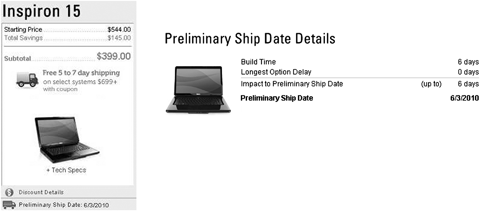
Table 1 shows FedEx, a logistics firm, adopting DQM, and Figure 1 shows Dell, a make‐to‐order computer manufacturing firm, adopting UQM. When customers send packages by FedEx, they are offered a menu of delivery lead times and prices to choose from. When the delivery lead time is shorter, the price is naturally higher. In Figure 1, Dell customers are all quoted the same single price and manufacturing lead time.

Table 1

Delivery Lead Time and Price Menu from the FedEx Website

Service	Delivery commitment	Rate (US$)
FedEx First Overnight	8.00am or 8.30am the next business day to major cities	131.98
FedEx Priority Overnight	10.30am the next business day to most cities	103.86
FedEx Standard Overnight	3.00pm the next business day to most cities	95.03
FedEx 2Day	4.30pm in 2 business days to most cities	64.37
FedEx Same Day	Same day in shortest time possible. Call 1 800 Go FedEx for availability and rate

Figure 1

Example of Price and Ship Date Quotation from Dell's Website

In practice, both quotation modes are popular. Ameristock (http://www.ameristock.com) follows UQM by quoting a 10‐second maximum trading time per internet equity trade to all customers. In contrast, Target uses DQM for its film printing services. Regular film printing takes a day and customers pay US$4.99 per roll. But, for US$5.99 per roll, their photos are delivered within an hour. Similarly, Plantgel (http://www.plantgel.com), a firm selling nutrition gels for plants, takes about 10 days to process and handle a regular order. But for US$3 more, this time is cut to a day. Because both quotation modes are commonly observed, how should a firm decide which one to adopt and under what circumstances? This question motivates our study.

DQM is beneficial if customers are heterogeneous in their valuation for lead time. Blackburn et al. (1992) and Smith et al. (2000) note that customers can often be classified into two segments: price sensitive (PS) and lead time sensitive (LS). LS customers value lead time reduction more than PS customers. The value of one unit lead time reduction is called the delay cost rate in the literature (Afeche 2006, Van Mieghem 2000).

Different customer types, i.e., customer heterogeneity, can result from individual and situational characteristics. For example, if a customer needs a laptop for a project with a tight deadline, then the customer is LS and is willing to pay more for lead time reduction. In another scenario, if a customer sees a digital camera on promotion and places an order for it despite having no immedate need, the customer is PS.

Thus, customers can be characterized by their valuation for the product and their delay cost rate. The product valuation is the maximum willingness‐to‐pay given no delay. The delay cost rate shows how urgently a customer wants the good. Clearly, a LS customer has a higher delay cost than a PS customer.

Customer types are private information. However, a firm using DQM can infer customer types from their choices. When a firm designs a proper menu, customers reveal their type by self‐selecting the option designed for their type, i.e., customers who choose the regular (respectively, express) service option in the menu are PS (respectively, LS). To design a menu for customers to reveal their types is called mechanism design (Fudenberg and Tirole 1991). Revelation of customer type information is costly because the firm gives extra benefits, called information rent, to motivate customers to choose the options intended for their types. However, DQM enables a firm to benefit from price discrimination. By providing express service, a firm can extract more revenue from LS customers than in UQM.

Moving from demand side to production side issues in the UQM–DQM decision, clearly differentiated services raise operational complexity in a firm. It is important for firms to meet their lead time promises. Firms need to carefully evaluate and design their operations to ensure that goods are delivered on time. If they provide differentiated services through a shared priority queue, then they need to control admission and production priority of orders. This increases overhead cost and operating cost. But having different operating queues means additional capacity investment.

A question for firms that prefer DQM is whether express and regular services should share a priority queue or use different queues? Both are observed in practice. For example, FedEx uses different facilities for express and ground services, while UPS delivers express and ground services through one integrated network. As noted in Ata and Van Mieghem (2009), FedEx states, “We strongly believe that the optimal way to serve very distinct market segments, such as express and ground, is to operate highly efficient, independent networks with different facilities, different cut‐off times and different delivery commitments.” UPS claims, “Our integrated air and ground network enhances pickup and delivery density and provides us with the flexibility to transport packages using the most efficient mode or combination of modes.”

This paper examines dedicated capacities for differentiated services. Afeche and Mendelson (2004) compare providing uniform service and differentiated services through priority auction using shared capacity. Under their problem settings, they concluded that providing differentiated services is always better than providing uniform service. On the other hand, the comparison of UQM and DQM in a queueing setting for a company that performs differentiated services through different queues, as many firms in industry do (Boyaci and Ray 2003), is understudied. Our study focuses on those companies that perform different services via dedicated capacities. Our paper complements the literature by filling this gap.

Our analytical models determine the optimal prices, lead times, capacity levels, and optimal profits under each quotation mode. We compare the optimal profits to gain the critical managerial insights as to which quotation mode a firm should use. We find that DQM is dominated by UQM whenever PS customers have positive utilities in UQM or LS customers have positive utilities in DQM. A summary of our results from the perspective of customer characteristics follows:

If LS customers do not value the product more than PS customers, then UQM is more profitable than DQM, independent of the proportion of LS customers in the market or how expensive it is to provide the product.

If LS customers value the product more than PS customers, then the optimal quotation mode depends on the difference between delay cost rates of LS and PS customers. If LS customers' delay cost rate is even slightly larger (made precise in section 5), then again UQM is better than DQM.

Otherwise, the decision depends on the proportion of LS customers in the market and how expensive it is to provide the product to customers.

We conducted sensitivity analyses for optimal lead time, price, and capacity level decisions on marketing parameters such as customer product valuation, customer delay costs, proportion of LS customers in the market, and operating parameters such as service level (lead time reliability) and capacity cost. The effects of these parameters on the differentiation level between express and regular service options are also analyzed.

The paper is structured as follows: after reviewing literature in section 2, the model framework is introduced in section 3, then UQM and DQM are compared for three scenarios in sections 4–6. We perform some numerical analysis in section 7 and conclude in section 8.

2. Literature Review

DQM can be traced back to the price‐quality screening problem in economics, where a firm designs an optimal price‐quality menu and learns a customer's type from his/her choice. Lead time is an important indicator of service quality. When lead time is shorter, service quality is higher. So the price‐lead time menu in an optimal DQM is similar to a price‐quality menu in economics. In section 2.1, we review the price‐quality screening problem in economics.

In section 2.2, we survey papers studying price and lead time quotation. These papers consider a queueing operational environment and can be classified into two major categories: dynamic quotation, where the quoted lead time to a customer changes dynamically according to the status of the queue at the moment when the customer arrives, and stationary quotation, where the quoted lead time is predetermined when designing the production or service system and is the same to all customers arriving over time. Under stationary quotation, we further classify papers into UQM and DQM, which itself includes two segments: papers considering shared capacity to provide differentiated services and papers considering dedicated capacities. We position our paper as one of the very few papers that compare uniform and DQMs to decide the best quotation mode for a company.

2.1. Price‐Quality Screening Problem

The differentiated lead time and price quotation mode is closely related to the classical price‐quality screening problem in economics. Mussa and Rosen (1978) is the first paper on price‐quality design for a multi‐product monopoly. It and several follow‐up studies, e.g., Besanko et al. (1987), assume a continuum of customer types with unit demand. Customer utilities are functions of some customer attribute, product or service quality, and price. The customer attribute is private information about a customer, such as his or her product valuation. It is distributed over some interval according to a continuous distribution. Customer utility function is increasing and concave in the quality level. The problem is to choose a price‐quality menu to maximize expected profit subject to customers' choice behaviors. Rochet and Chone (1998) generalize the analysis of Mussa and Rosen (1978) to the case of multidimensional customer types. Rochet and Stole (2003) provide a recent survey on the economics of screening.

Our paper differs from the price‐quality screening literature in the following ways. First, this economics literature does not consider operational issues. However, in our study, a firm considers both production and marketing aspects when designing the optimal price‐lead time menu in DQM. In order to maintain the reputation of reliable lead time quotation, firms decide simultaneously on prices, lead times, and capacity levels. Second, our focus is to identify situations where UQM is better than DQM or vice versa, while the price‐quality screening literature focuses on designing a price‐quality menu that maximizes profits for a firm.

2.2. Lead Time and Price Quotation

The lead time and price quotation literature can be separated into two major categories: dynamic quotation and stationary quotation. Examples of papers studying dynamic quotation are Duenyas and Hopp (1995), Webster (2002), Plambeck (2004), and Ata and Olsen (2009). We focus on stationary quotation.

Under stationary quotation, papers can be classified into UQM or DQM. Some papers that investigate the optimal stationary lead time and price quotation for a UQM are Palaka et al. (1998) and So and Song (1998), who model a firm as a single server queue and provide the optimal values of service rate, price, and lead time. They maximize a firm's profit while satisfying service level constraints. So (2000) extends So and Song (1998) to include competition among firms. Ray and Jewkes (2004) evaluate the changes in the optimal lead time values in a UQM when price is not a decision variable but an explicitly specified function of lead time. Rao et al. (2005) developed a model to integrate demand and production planning, which determines an optimal production planning interval and the corresponding optimal uniform lead time quotation. Easton and Moodie (1999) study UQM for a make‐to‐order firm to bid on contingent project contracts considering competition of bidders.

Our UQM also aims to maximize profits under service level constraints in a queueing setting, but differs from the above UQM studies by considering customer behavior. We incorporate a customer utility maximization process into a firm's profit maximization decision‐making process.

Other research in uniform lead time and/or price quotation takes the perspective of coordination between marketing and operations (e.g., Balasubramanian and Bhardwaj 2004, Dewan and Mendelson 1990, Erkoc et al. 2008, Ho and Zheng 2004, Pekgün et al. 2008). These model the marketing and operations departments in a firm as independent decision makers. Price is decided by marketing and lead time is decided by operations. These papers focus on how to adopt coordination mechanisms to decrease the inefficiency caused by decentralization of price and lead time decisions. In contrast, we model firms that can make centralized decisions.

The differentiated lead time and price quotation literature can be further classified according to the following four fundamental problem characteristics: (1) the problem is to design an optimal price‐lead time menu in a market with heterogeneous time‐sensitive customers, (2) a firm cannot observe customer types and customers can choose among all available service options, (3) the optimization objective is to maximize the firm's profits or revenues instead of system or social benefits, and (4) companies use dedicated capacities for different services instead of using priority control over shared capacity to provide differentiated services. Table 2 provides a summary for the stationary DQM literature.

Table 2

Stationary DQM Literature

Characteristics	Mendelson and Whang (1990)	Van Mieghem (2000)	Maglaras and Zeevi (2005)	Boyaci and Ray (2003)	Afeche (2006)	Katta and Sethuraman (2005)	This study
Heterogeneous customers	X	X	X	X	X	X	X
Private information of customer type	X	X		X	X	X	X
Revenue maximization			X	X	X	X	X
Dedicated capacities				X			X

The DQM in our paper extends Boyaci and Ray (2003) to incorporate a customer utility maximization decision‐making process into a firm's profit maximization decision‐making process. In addition, we have a different research focus from Boyaci and Ray (2003). We study the conditions for UQM to be better than DQM or vice versa while Boyaci and Ray (2003) focus on designing the optimal DQM menu.

There are very few papers in the literature that study the conditions for UQM to outperform DQM or vice versa. Some studies note that UQM may outperform DQM. For example, Afeche (2006) and Katta and Sethuraman (2005) note that it can be beneficial to pool customers of different types together and treat them equally. To the extent that a priority auction can provide differentiated prices and service levels to different customers, Afeche and Mendelson (2004) is close to our study. They compare UQM with priority auction and show that priority auction always dominates UQM.

3. Problem Setting and Models

In this section, the production and market/customer settings are discussed. Second, models for both UQM and DQM are developed. Table 3 lists the notation used.

Table 3

Notation

Decision variables
L _i=	Lead time in the option intended for type i customers; i∈{p, l}
P _i=	Price in the option intended for type i customers; i∈{p, l}
μ_i=	Service rate of a production queue serving type i customers; i∈{p, l}; μ _p<μ _l
Parameters concerning customers and market
λ=	Customer arrival rate
θ=	Proportion of LS customers among all arrived customers; 0<θ<1
ν _i=	Product valuation of type i customers; i∈{p, l}
β _i=	Delay cost per unit time (delay cost rate) of type i customers, β _p<β _l
Parameters concerning production
α=	Desired lead time reliability predetermined by managers; 0<α<1
M=	Capacity cost parameter
m=	Variable production cost for one unit of product
k≡	−Mln (1−α); service cost parameter

Customer arrivals are modeled as a Poisson process with rate λ customers per unit time. Among these λ customers, proportion θ are LS and 1−θ are PS, where 0<θ<1. By the properties of a Poisson process, the arrival of LS customers forms a sub‐Poisson process with rate λθ. PS customers also form a sub‐Poisson process with rate λ(1−θ). We assume unit demand per person.

Whether an arrived customer places an order depends on the utility value that he or she gets from buying. To model customer behavior and preferences about lead time and price, we use a linear utility/surplus function for each customer segment, where upper case L and P are lead time and price, and lower case subscripts l and p represent LS and PS customer segments. The parameter v _i represents customer valuation of the product that he/she may buy. It is also the maximum amount of money that a customer is willing to pay for a product when lead time L=0. The delay cost rate β _i measures how urgent a customer wants the product or service to be completed. With one unit time (e.g., 1 day) delay, the customer incurs β _i dollars loss. Obviously, LS customers have a higher delay cost rate than PS customers, i.e., β _l>β _p.

From the production perspective, a firm needs to determine its chosen production capacity level, such as the daily production volume. A lead time reliability target α is set by managers. That is, the probability, Prob{actual lead time > quoted lead time}, should not exceed 1−α.

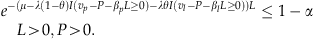
In the UQM, similar to So and Song (1998), the production system is an M/M/1 queue with a service rate μ, which is a decision variable to determine a firm's capacity level. In an M/M/1 queue, the actual lead time, i.e., the waiting time plus the service time in the queue for a customer, follows an exponential distribution. Considering a quoted lead time L in the UQM, we have the following lead time reliability (service level) constraint: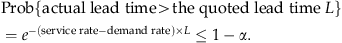

Abate et al. (1996) show that when the service level α is high, the distribution of the actual customer lead time in a G/G/s queue is well approximated by the exponential distribution in an M/M/1 queue. Thus, our lead time reliability constraint would also be approximately valid for general demand and service rate settings as in a G/G/s queue.

When a firm adopts a DQM, two options are provided to customers: regular service with price P _p and lead time L _p, targeted to PS customers, and express service with price P _l and lead time L _l, targeted to LS customers. In a dedicated capacity system, regular and express services are fulfilled in separate production systems, i.e., two M/M/1 queues, each having different service rates. The express queue has a service rate μ _l and the regular queue has a service rate μ _p, where μ _l>μ _p. 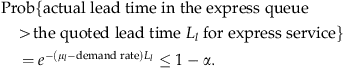To ensure that the firm achieves its lead time reliability target in each queue, service rates have to be large enough so that the following constraints are satisfied for the two M/M/1 queues: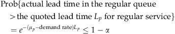

Costs are split into production and capacity costs. When producing a product, a firm incurs production costs, including material costs. The variable production cost to produce one unit of product is a constant m.

Capacity cost includes investments in buildings, equipment, and employees to operate and maintain a facility. Since these resources are shared by all products produced in the firm, capacity cost should also be shared by all products. We introduce a capacity cost rate that includes two parts: employee wage rate and depreciation rate of facilities. Clearly, when service rate μ is larger, the firm incurs a higher capacity cost rate. For simplicity of computation, we assume that the capacity cost rate is a linear function Mμ, where M is a positive constant, denoted as the capacity cost parameter. The value of M shows how expensive it is to increase the capacity level (service rate) in the firm.

Depending on how the capacity of a queue is built, a firm can have different capacity cost parameters for an express queue and a regular queue. For example, in the logistics industry and other highly automated industries, an express queue builds capacity through advanced and expensive equipment, e.g., FedEx Express uses airplanes while FedEx ground uses trucks. Then the express queue may have a higher capacity cost parameter than a regular queue.

However, in some industries, capacity is increased by adding more workstations in a modular manner. Each module has the same cost. Thus an express queue and regular queue would then have the same capacity cost parameters. For example, airlines usually have express and regular check‐in queues. The service rate of each queue increases with the number of counters serving each queue. The cost to build and operate one counter may be the same for an express queue and a regular queue.

To establish a baseline, we assume that the express queue and regular queue both have the same capacity cost parameter M. We later discuss the implications of relaxing this assumption. We also show that major results remain the same even when M is different for each queue.

3.1. Models for the UQM

We consider three scenarios for the UQM, each depending on different marketing strategies. These scenarios are labeled as LS Focus (the firm targets primarily LS customers), PS Focus (the firm targets primarily PS customers), and Pooling (the firm targets both segments). Each scenario has a different objective function and different constraints.

In all cases, the objective is to maximize profit rate, i.e., the average profit per unit time, which equals the revenue rate minus variable cost plus capacity cost rates. Both the revenue and cost rates depend on the demand rate. We consider the demand rate first.

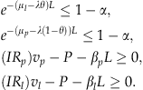
In the UQM, after an arrived customer is quoted a lead time and price, whether he/she places an order is decided by the customer's utility function value of the quoted lead time and price. Normalizing the maximum utility obtained from other companies to zero, customers place orders when the lead time and price quotation gives them nonnegative utility, which is the individual rationality (IR) condition. Considering the utility function, U _i(L, P)=v _i−P−β _i L, i∈{l, p}, the IR condition for type i customers is v _i−P−β _i L≥0, i∈{l, p}.

In the LS Focus UQM, the quoted lead time and price combination satisfies the IR condition for LS customers only, i.e., v _l−β _l L−P≥0 and v _p−β _p L−P<0. Only LS customers buy. The demand rate is λθ and the revenue rate is Pλθ.

We do similar analyses for both the PS Focus UQM and the Pooling UQM. Table 4 lists the models for the UQM under each scenario.

Table 4

Models for the UQM

LS Focus uniform	PS Focus uniform	Pooling

Subject to	Subject to	Subject to
e ^{−(μ−λθ)L}≤1−α	e ^{−(μ−λ(1−θ))L}≤1−α	e ^{−(μ−λ)L}≤1−α
v _l−β _l L−P≥0	v _l−β _l L−P<0	v _l−β _l L−P≥0
v _p−β _p L−P<0	v _p−β _p L−P≥0	v _p−β _p L−P≥0
L>0, P>0	L>0, P>0	L>0, P>0

All three cases for UQM can be integrated into one model by introducing an indicator function I(x), where I(x)=1 if x is true and I(x)=0 if x is false. The integrated model for the UQM is as follows: 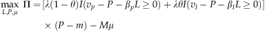subject to 1

When the IR condition for PS customers is satisfied, I(v _p−P−β _p L≥0)=1 so that the firm gets demand from PS customers. Similarly, only if the IR condition for LS customers is met, I(v _l−P−β _l L≥0)=1 and LS customers buy from the firm. Hence, the expression λ(1−θ)I(v _p−P−β _p L≥0)+λθI(v _l−P−β _l L≥0) measures the total demand rate for the firm. Based on this demand rate, the objective function represents the total profits from serving customers and constraint (1) guarantees the lead time reliability and service level α.

As noted in So and Song (1998), the lead time reliability constraint in each model should be binding at optimality. This is intuitive. In order to maximize the objective functions, the service rate μ should be as small as possible. However, the lead time reliability constraint gives the lower bound for the service rate μ in each model. Therefore, this constraint should be binding at optimality, which specifies the following optimal service rate for the integrated UQM. 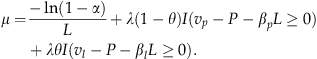2

As a result, the objective of a firm following the UQM is to maximize total profit with capacity level as given in Equation (2). That is, the integrated model for the UQM can be rewritten as follows: 3 subject to L>0, P>0.

3.2. Model for the DQM

DQM requires an application of mechanism design. According to the revelation principle (Fudenberg and Tirole 1991), a menu where both LS and PS customers reveal their true types by choosing the right options is optimal for the firm. Therefore, in DQM, a firm quotes a menu {(L _p, P _p), (L _l, P _l)} to customers with the intention that LS customers select the express service option (L _l, P _l) and PS customers choose the regular service option (L _p, P _p). To achieve this goal, besides the previous individual rationality conditions, LS customers should get more utility from option (L _l, P _l) than option (L _p, P _p) and vice versa for PS customers, which is the incentive compatibility (IC) condition (Fudenberg and Tirole 1991). Considering the utility function, U _i(L, P)=v _i−P−β _i L, i∈{l, p}, the IC condition requires the following:

When the quoted options (L _p, P _p) and (L _l, P _l) satisfy the IR and IC constraints, all arrived PS and LS customers should place orders with the options (L _p, P _p) and (L _l, P _l), respectively. Hence, the demand rate is λθ for express service option (L _l, P _l) and λ(1−θ) for regular service option (L _p, P _p). Therefore, the revenue rate is λθP _l+λ(1−θ)P _p in the DQM. 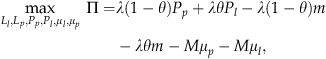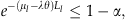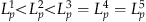The model is as follows: subject to 4 5 6 7

Constraints (4) and (5) are the lead time reliability constraints for the express queue serving LS customers and the regular queue serving PS customers, respectively. Constraints (IR _p) and (IC _p) ensure that PS customers select the regular service option (L _p, P _p). Constraints (IR _l) and (IC _l) ensure that LS customers select the express service option (L _l, P _l). Constraints (6) and (7) require that the lead time is shorter and thus the price is higher in the express service option than in the regular service option.

Similar to the argument for the UQM in section 3.1, the lead time reliability constraints should be binding at optimality. Hence, the service rates for each queue are 8 9

As a result, the objective of a firm following the DQM is to maximize total profit with capacity levels as given in Equations (8) and (9). So the model for the DQM can be rewritten as follows: 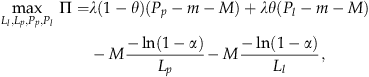10 subject to (IR _p), (IR _l), (IC _p), (IC _l), (6), and (7).

4. When LS Customers Value the Product No More than PS Customers

In practice, it may happen that sometimes LS customers do not value the product or service more than PS customers, i.e., v _l≤v _p. For example, a student and a professional software engineer may both order the same computer from Dell. The student needs the computer now for the coming semester and may choose next‐day delivery. The professional software engineer is not in a hurry to receive the computer and may choose 3–5‐day delivery. Obviously, the poor student is a LS customer but the rich software engineer is a PS customer. Now if Dell increases the price for the computer, it may happen that the software engineer is still willing to buy the computer but the student may not be willing to buy it any longer and may shop elsewhere. This example shows that a PS customer may have a higher product valuation than an LS customer.

Theorem 1. When LS customers do not value the product more than PS customers, the Pooling UQM is always better than the DQM in terms of profits. This result is independent of customer delay costs, proportion of LS customers, service level, and capacity cost. 

Proofs of all theorems and propositions are in the online Appendix.

Remark 1. Even if the capacity cost parameter M is close to zero, the result still holds. When M is very small, the operational disadvantage of DQM vanishes. This implies that the informational disadvantage of DQM takes all responsibility for this result. 

When v _l≤v _p, LS customers do not value products more than PS customers. Intuitive understanding for this scenario is that LS customers are not willing to pay more than PS customers, but they are more picky about lead time than PS customers. So the express service option that LS customers are willing to buy will also look good to PS customers. The firm has to lower the price for the regular service in order to dissuade PS customers from choosing the express service option under DQM. In this case, the decrease of revenue from PS customers cannot be justified by the extra gain from LS customers. So DQM is dominated by UQM in this case.

5. When v _l>v _p and LS Customers' Delay Cost Rate is Only Slightly Larger than PS Customers' Delay Cost Rate

When LS customers have a higher product valuation than PS customers, i.e., v _l>v _p, which quotation mode is better depends on the percentage of LS customers' delay cost rate exceeding PS customers' delay cost rate. In this section, we focus on the situation where , i.e., . The situation where is examined in section 6.

To illustrate the situation, consider the online make‐to‐order furniture industry, which usually has a long manufacturing and shipping lead time. Customers choose to buy from online make‐to‐order furniture companies for several reasons. For example, price may be cheaper than local stores or a customer may value a customized style of the furniture. If a customer buys mainly because of the former reason, then she is a PS customer. She is an LS customer for the latter reason. Obviously, LS customers value the product more than PS customers. In terms of delay cost, PS customers are more reluctant to pay more to reduce lead time than LS customers because PS customers care more about money. However, considering the long lead time in the make‐to‐order furniture industry and both LS and PS customers' are willing to wait for such a long lead time rather than buy finished products at a local store, both LS and PS customers may have small delay costs although LS customers are willing to pay more to reduce lead time than PS customers. The difference between their delay costs may be much smaller than the difference between their product valuation, i.e., .

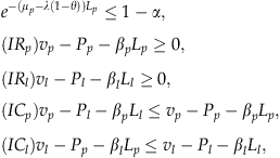
When v _l>v _p and , in the Pooling UQM, the IR condition for PS customers is binding at optimality. Thus the IR condition for LS customers is redundant. So P=v _p−β _p L at optimality. From Equation (2), we have the following objective function for the Pooling UQM. 11

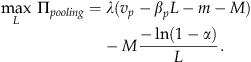
Under the DQM, the IR condition for PS customers and the IC condition for LS customers should be binding at optimality while the other two IR and IC conditions are redundant. Therefore, P _p=v _p−β _p L _p and P _l=β _l(L _p−L _l)+v _p−β _p L _p. The objective function (10) for the DQM is transformed as follows: 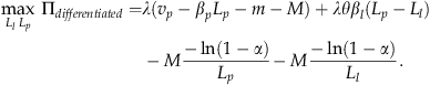12

As mentioned in the introduction, DQM has two disadvantages compared with UQM. One is from asymmetric information, where a firm incurs some cost to motivate customers to self‐select the right options intended for them to choose. Because v _l>v _p, LS customers are willing to pay more than PS customers, and compared with the difference between their product valuations, LS and PS customers have relatively similar delay cost rates. So the regular service option that is intended for PS customers will also look attractive to LS customers. In order to dissuade LS customers from choosing regular service, the firm charges a lower price for express service than what LS customers are willing to pay. (This ``lower price” is higher than the price charged for the regular service.) In this paper, we refer to the amount of revenue reduction (caused by the price reduction) as information cost because price reduction would not happen if the firm knows information about each customer's type. We feel that the term information cost may be more meaningful to a manager than the traditional economic term, information rental.

Another disadvantage of DQM is from the operational complexity to provide differentiated services to customers. Because firms in our study implement differentiated services through dedicated capacities, this disadvantage is transformed to additional capacity costs.

Comparing objective function (11) for Pooling UQM and objective function (12) for DQM gives some insights on the tradeoffs to consider when following a DQM. The second term λθβ _l(L _p−L _l) in (12) is the extra profits from LS customers after deducting the information cost. The last term illustrates the additional capacity cost incurred under the DQM when adding an express service option to form a DQM menu.

Remark 2. The additional capacity cost increases with M and α but decreases with L _l . This is because a firm needs more capacity to achieve its service promise when it guarantees a high service level α or quotes a short lead time L _l for express service. This implies that a firm setting a high service level (α is high), requiring expensive capacity investment (M is large), or promising short lead times to LS customers (L _l is small), experiences large disadvantage on capacity costs when following DQM.

Theorem 2. If LS customers value products more than PS customers and LS customers' delay cost is only slightly larger than PS customers' delay cost, i.e., , then the pooling UQM is always better than the DQM. This result is independent of the proportion of LS customers in the market, service level, and capacity cost. 

To better illustrate the tradeoffs, we conduct the following analyses to isolate the operational disadvantage and informational disadvantage. Our analyses show that UQM may or may not outperform DQM depending on certain parameter values when either capacity cost or information cost disadvantage disappears under DQM.

5.1. DQM Under Full Information

We analyze the first‐best solution for DQM, which provides an upper bound on the performance of DQM with asymmetric information. With full information, a firm knows each customer's type so that there is no information cost in DQM. Compared with UQM, the only disadvantage of DQM is from additional capacity cost.

When a firm knows each customer's type, it can select the service option for each customer according to his or her type. Customers either take it or leave it. So IC conditions are unnecessary in DQM. Furthermore, the firm charges exactly what a customer is willing to pay. So individual rationality conditions are binding at optimality. Hence, P _p=v _p−β _p L _p and P _l=v _l−β _l L _l. The objective function (10) for DQM becomes: 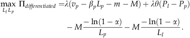13

The difference between objective function (13) under full information and (12) under asymmetric information quantifies the information cost in DQM under asymmetric information. The second term λθ(P _l−P _p) in (13) is the only difference with (12). It is equivalent to λθ(v _l−β _l L _l−v _p+β _p L _p) since P _p=v _p−β _p L _p and P _l=v _l−β _l L _l. Comparing the second terms in objective functions (13) and (12), we quantify the information cost as λθ(v _l−v _p)−λθL _p(β _l−β _p).

Remark 3. Information cost increases with the production valuation difference between the two customer types and decreases with the delay cost rate difference between the two types. This implies that information cost is high when the LS customers' delay cost rate is just slightly larger than PS customers' delay cost rate, i.e., . Also information cost decreases with the lead time L _p quoted in the regular service option. This is because when L _p increases, the regular service option is less attractive to LS customers. Then information cost can be low since LS customers are already highly motivated to choose express service because of the long lead time of regular service. 

Maximizing the objective function (13) gives the following optimal solutions: 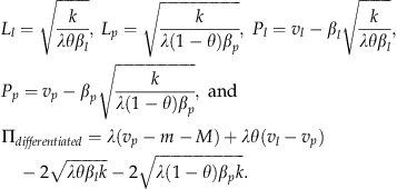14

The optimal lead time L _p under asymmetric information is longer than the one under full information. This is because a long L _p helps a company to reduce the information cost under asymmetric information.

Solving the uniform pooling model gives the optimal profit as follows: 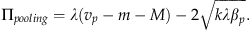15

Comparing (15) and (14), we see no dominant relationship under full information. Which quotation mode is better depends on the proportion of LS customers in the market, customer valuations for the product or service, capacity cost, and service level in a firm.

5.2. Providing Uniform Service with Two Queues

To compare UQM and DQM in the same operational environment, we perform uniform service with two queues. Suppose that one queue handles demand from LS customers with service rate μ _l. The other queue deals with PS customers with service rate μ _p. Then the pooling UQM is modified to: subject to

Similarly, the two lead time reliability conditions are binding at optimality. The IR condition for PS customers is also binding at optimality, which implies that the IR condition for PS customers is redundant. So the objective function can be transformed to: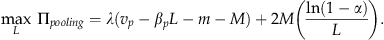

Maximizing this objective function gives the following optimal values. 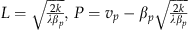, and .

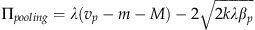Comparing the optimal profits from UQM and DQM, 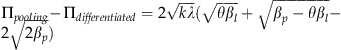. This shows that which quotation mode is better depends on the proportion of LS customers and the delay cost rates of customers. So the UQM may or may not outperform the DQM if the disadvantage from capacity cost is eliminated for the DQM.

6. When v _l>v _p and LS Customers have a Much Larger Delay Cost Rate than PS Customers

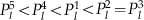
In this section, we study the situation where LS customers value the product or service more than PS customers and they are also differentiated from PS customers with a much higher delay cost rate, i.e., . First, the optimal solutions for the uniform and DQMs are presented. Then the optimal profits generated from these two quotation modes are compared to show the conditions under which DQM is better than UQM. Finally, numerical experiments are conducted to illustrate the effects of parameter changes on a firm's quotation mode decision.

Such a situation where v _l>v _p and is commonly observed in practice, especially in industries offering a short manufacturing and shipping lead time. For example, in the film printing service industry such as a Target or Walmart film printing service center, LS customers may have a much higher delay cost rate than PS customers. For another example, in the warehouse industry, LS customers placing express packing and picking orders have a much more expensive delay cost rate than PS customers.

In order to solve the models, we first introduce the zero utility indifference curve for customers. Indifference curves can be drawn to show all combinations of lead time and price that yield the same level of utility for customers. By setting the utility function values to zero, we get zero utility indifference curves AB and CD for LS and PS customers, respectively, as shown in Figure 2.

Figure 2

Indifference Curves with Zero Utility Values

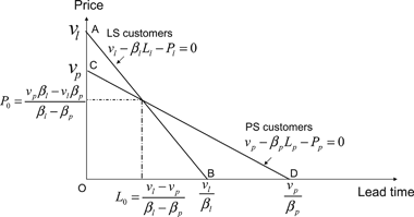
Because LS customers have a larger delay cost than PS customers, i.e., β _l>β _p, the indifference curve for LS customers has a larger slope than the curve for PS customers as shown in Figure 2. Because , . Together with v _l>v _p, this implies that there exists a single crossing point, denoted (L ₀, P ₀), where L ₀=(v _l−v _p)/(β _l−β _p) and P ₀=(v _p β _l−v _l β _p)/(β _l−β _p).

For lead times shorter than L ₀, LS customers are willing to pay more than PS customers. However, we allow for the possibility that LS customers may want to pay less than PS customers if the lead time is very long (longer than L ₀ in Figure 2). For example, if a customer needs a laptop for a project with a tight deadline, the customer is LS and is willing to pay more to get the laptop before the deadline. However, if the quoted lead time is too long for the LS customer to get the laptop before the deadline, he is only willing to pay less than a PS customer because, for example, missing the deadline has a high disutility for the LS customer.

6.1. Optimal UQMs

From section 5, k≡−Mln(1−α). The value of k indicates how expensive it is for a firm to quote short lead times to customers. It is determined by two factors: M (the capacity cost parameter indicating how expensive it is to increase the capacity level) and α (the service level requirement). When capacity is expensive to acquire (M is large) and/or the predetermined service level is high (α is large), the firm has a large k value. Then it may not be profitable to quote short lead times to customers. Therefore we label k as service cost parameter since it indicates how expensive it is to provide high quality service (short lead times with high reliability) to customers.

Proposition 1. The profit‐maximizing lead time and price quotations (L, P) under LS Focus, PS Focus, and Pooling UQMs are as described in Table 5 . 

Table 5

Optimal Lead Times and Prices in the UQMs

Name	Optimal service rate, lead time, price, and related profit
LS Focus	If , then



PS Focus	If , then



Pooling	(Case 1: LS customers have positive utilities)	(Case 2: PS customers have positive utilities)	(Case 3: no customers have positive utilities)
	If ,	If ,	If ,
	then	then	then
			L=L ₀
			P=P ₀

Note that some cases of LS Focus and PS Focus UQMs are omitted in Table 5 because they are always dominated by Case 3 of the Pooling UQM in terms of profits. In the omitted cases, the conditions for Case 1 of LS Focus or PS Focus in Table 5 are not satisfied and the optimal solution is to charge P=P ₀ and quote L=L ₀. Next, we analyze the sensitivity of optimal solutions to parameters.

As can be seen from Table 5, when parameter k increases, the cost for a short lead time increases. So firms prefer to quote a long lead time with a low price to customers. Table 6 summarizes how the optimal solutions change when increasing a parameter's value.

Table 6

Sensitivity Analyses for UQMs

Parameter name	Optimal lead time					Optimal price					Optimal service rate					Optimal profit
	LS	PS	Pooling			LS	PS	Pooling			LS	PS	Pooling			LS	PS	Pooling
	(1)	(1)	(1)	(2)	(3)	(1)	(2)	(1)	(2)	(3)	(1)	(1)	(1)	(2)	(3)	(1)	(2)	(1)	(2)	(3)
α	+	+	+	+	=	−	−	−	−	=	+	+	+	+	+	−	−	−	−	−
M	+	+	+	+	=	−	−	−	−	=	−	−	−	−	=	−	−	−	−	−
k	+	+	+	+	=	−	−	−	−	=	?	?	?	?	?	−	−	−	−	−
θ	−	=	=	=	=	+	−	=	=	=	+	−	=	=	=	+	−	=	=	=
β _l	−	=	=	−	−	−	=	=	−	+	+	=	=	+	+	−	=	=	−	−
β _p	=	−	−	=	+	=	−	−	=	−	=	+	+	=	−	=	−	−	=	−
v _l	=	=	=	=	+	+	=	=	+	−	=	=	=	=	−	+	=	=	+	+
v _p	=	=	=	=	−	=	+	+	=	=	=	=	=	=	+	=	+	+	=	+

Increase (+), decrease (−), unaffected (=), ambiguous (?).

6.2. Optimal Differential Quotation Modes

The DQM consists of three major cases, with three subcases under each major case. Different IR and IC constraints can be binding at optimality in each case. For example, if the solutions of L _l and L _p from the first order conditions satisfy 0<L _l<L _p<L ₀, then similar to section 5, the IR condition for PS customers and the IC condition for LS customers are binding at optimality, i.e., LS customers have positive utilities. In order to assure that 0<L _l<L _p<L ₀, we have conditions on k and θ for this case to happen. The other two cases are 0<L _l<L ₀<L _p and L ₀<L _L<L _p. If 0<L _l<L ₀<L _p, then the IR conditions for PS and LS customers are binding, i.e., no customers have positive utilities. If L ₀<L _L<L _p, then similar to section 4, the IR condition for LS customers and the IC condition for PS customers are binding, i.e., PS customers have positive utilities. Considering that (L _l, P _L) or (L _p, P _p) may also be at the crossing point (L ₀, P ₀), we have five cases in total. The details of the process to get these solutions are in the online Appendix. We now present the solutions.

Proposition 2. The profit‐maximizing lead time and price quotations (L _p, P _p ) and (L _l, P _l ) under DQM are given in Table 7 . 

Table 7

Optimal Lead Time and Price Options in the DQM

Case 1: LS customers have positive utilities	Case 3: no customers have positive utilities	Case 5: PS customers have positive utilities
If and , then	If , , and , then	If , , and , then





Case 2: no customers have positive utilities	Case 4: no customers have positive utilities
If , , and , then	If , , , and , then
	L _l=L ₀
	P _l=P ₀
L _p=L ₀
P _p=P ₀
	.

Fix customer arrival rate (λ), production valuation (v _i), and lead time reduction valuation (β _i). Then the case in Table 7 that a firm should choose to design its optimal DQM only depends on two factors: the proportion of LS customers θ and the service cost parameter k, which indicates how expensive it is to quote short lead times to customers. We can illustrate the suitable region specified by parameters k and θ for each case (listed in Table 7) in Figure 3. If the values of k and θ fall in shaded region (1), (2), (3), (4), or (5), then Case 1, 2, 3, 4, or 5 in Table 7, respectively, is the optimal DQM that a firm should use. Otherwise, DQM is infeasible. According to our definition of DQM, a DQM must have differentiated services for consumers to choose from and different type of consumers should choose different services. In some regions, a company cannot design such differentiated service options so that different types of consumers would choose different services. That is, such a mechanism does not exist. Therefore, we say DQM is not feasible in those regions. Then a company has to use UQM because DQM is not an option to them.

Figure 3

The Five Feasible Regions for the Five Cases in Table 7

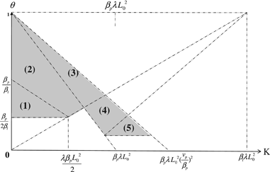
Figure 3 and Table 7 also provide the following three insights. First, when k is larger, lead times quoted in both options are larger. Second, when the proportion of LS customers θ increases, a firm surprisingly quotes a higher price in option (L _l, P _l) that is intended for LS customers to choose. Third, the difference in lead times of express service and regular service increases when it is more expensive to provide service to customers or when the proportion of LS customers increases. Fourth, let denote the lead time L _l quoted in Case i. Also denote other variables similarly. Then 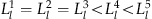, , , and .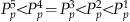

6.3. UQM and DQM Comparison

To determine which quotation mode is better for a firm, we first determine which optimal UQM listed in Table 5 is feasible in each of the five feasible regions for DQM in Figure 3. Only LS Focus and Pooling Case 1 are feasible UQM in regions (1) and (2). Three UQMs, LS Focus, PS Focus, and Pooling Case 1, are feasible in regions (3). In regions (4) and (5), besides PS Focus, Pooling Case 1 is feasible if , and otherwise, Pooling Case 2 is feasible. By comparing their profits, we have the following theorem.

Theorem 3 Whether a firm should adopt DQM or UQM depends on the firm's parameter values for k and θ.

If k and θ fall in region (1), UQM dominates DQM in terms of profits. Thus a firm should adopt UQM.

If k and θ fall in regions (2), (3), (4), or (5), there is no domination relationship between DQM and UQM.

If k and θ fall in any other regions, DQM is not feasible and thus a firm should adopt UQM.

When k and θ fall in region (1), Case 1 in Table 7 provides the optimal DQM. In region (1), the Pooling UQM Case 1 of Table 5 is also feasible and it generates more profits than the DQM Case 1. So pooling UQM is always better than DQM in region (1).

When k and θ fall in regions (2), (3), (4), or (5), DQM could be better than UQM or vice versa. The detailed conditions for DQM to generate more profits than UQM are specified in the online Appendix. Furthermore, in order to better understand the impact of parameter values on the choice of the optimal quotation mode, we provide numerical study in section 7. The numerical experiments show that Pooling UQM is slightly better than DQM when θ is small. DQM is much more attractive as θ increases. The numerical study also suggests that a firm's optimal quotation mode can switch from DQM to UQM when the difference between β _l and β _p decreases or the service level increases.

Comparing the optimal profits generated by UQM and DQM case by case leads to Table 8. Because each case has an applicable parameter region, “NA” is in the table when two cases cannot occur at the same time. For example, in the parameter region where the PS customers have positive utilities in the Pooling UQM, i.e., Case 2 in Table 5 is optimal for the Pooling UQM, k and θ must have fallen in the region where in Figure 3 and no DQM is feasible in this region. So “NA” is throughout the second row in Table 8. For another example, in the parameter region where LS customers have positive utilities in the DQM, i.e., Case 1 in Table 7 is optimal for the DQM, k and θ must have fallen in the region (1) in Figure 3. In this region, Case 1 in Table 5 is optimal for the Pooling UQM. So ``NA” is in the second and third rows for the first column of Table 8. This means that Cases 2 and 3 of UQM cannot happen if LS customers have positive utilities in the optimal DQM. Furthermore, “UQM” is in the table if the UQM generates more profits than the DQM. Otherwise, there is no domination relationship and we note “UQM or DQM” in the table.

Table 8

Comparison between UQMs and DQMs

Differentiated	Case 1: LS customers have positive utilities	Case 2: no customers have positive utilities	Case 3: no customers have positive utilities	Case 4: no customers have positive utilities	Case 5: PS customers have positive utilities
Pooling uniform
Case 1: LS consumers have positive utilities	UQM	UQM or DQM	UQM or DQM	UQM or DQM	UQM or DQM
Case 2: PS consumers have positive utilities	NA	NA	NA	NA	NA
Case 3: no customers have positive utilities	NA	NA	NA	UQM or DQM	UQM or DQM

From the perspective of customer utility, notice that LS (PS) customers have positive utilities in pooling Case 1 (2) as well as in differentiated Case 1 (5). Also note that when pooling Case 2 is optimal for UQM, DQM is not feasible and thus UQM is a company's only option. Correspondingly, the following theorem can be summarized from Table 8.

Theorem 4 When either of the following two scenarios occurs, a company should use UQM rather than DQM.

PS customers have positive utilities in the optimal pooling UQM.

LS customers have positive utilities in the optimal DQM.

Theorem 4 also holds for scenarios in sections 4 and 5. In section 4, PS customers have positive utilities in the optimal pooling UQM. In section 5, LS customers have positive utilities in the optimal DQM. In both sections, UQM dominates DQM. Therefore, Theorem 4 is applicable to all scenarios regardless of the relationship between v _l, v _p, β _l, and β _p.

According to our analysis in section 6.1, all companies having a larger k value than would give positive utility to PS customers in the pooling UQM. Therefore, Theorem 4.1 suggests that a company with a high k value should not use DQM. Since k=−Mln(1−α), a high k value could be caused by a high M or α value. Therefore, if a company has an extremely high service level α, then it should not use DQM. For example, in the pizza delivery industry, the service level α is usually very high. Some companies promise that if service level α is not 100%, i.e., a pizza is not delivered within its quoted lead time, then the pizza is free. In such industries, a company should not adopt DQM.

According to our analysis in section 6.2, when both k and θ values are small, then a company leaves LS customers with positive utility in DQM. Therefore, Theorem 4.2 indicates that a company with small k and θ values should not use DQM. That is, although it is cheap to provide short lead times with high reliability, i.e., k is small, it is still not wise to use DQM if the majority of the customers are PS customers, i.e., θ is low. For example, some online companies, such as Plantgel (http://www.plantgel.com) selling exclusive products and facing various customers, offer regular and express order handling and shipping services. However, this strategy may not be good for some other online companies such as Graveyardmall (http://graveyardmall.com/boxofstforfa.html), whose majority customers are PS customers, i.e., θ is small.

Next, we relax the assumption that the express queue and regular queue have the same capacity parameter cost M. If the express queue has a higher capacity cost parameter than M, DQM is even less attractive. So DQM Case 1 is again dominated by the Pooling UQM. DQM Case 2 to Case 5 could still be dominated by the Pooling UQM under certain conditions.

Hence Theorem 3 still holds after slightly modifying the conditions to reflect a different capacity cost parameter for the express queue. Theorem 4 is unchanged and the conclusions would be the same. That is, whenever PS customers have positive utilities in the optimal pooling UQM or LS customers have positive utilities in the optimal DQM, a firm should use UQM rather than DQM.

7. Numerical Examples

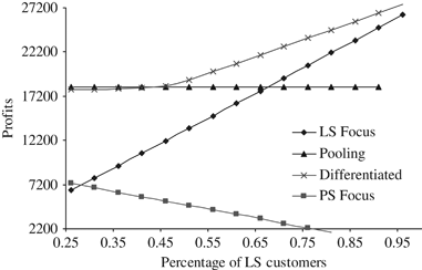
We now examine how a firm's quotation mode decision can change with the proportion of LS customers θ, capacity cost parameter M, gap between delay costs of LS and PS customers β _l−β _p, and service level α. Numerical examples are constructed to illustrate the optimal profits from UQM and DQM. A firm should choose the quotation that generates the highest profit. The following parameter values are used in the numerical examples: v _l=US$600, v _p=US$500, β _l=US$100/day, β _p=US$50/day, θ=0.3. Also, m=US$250, M=US$50, and α=95%.

To examine the impact of θ on a firm's quotation mode decision, the proportion of LS customers θ increases from 0.25 to 0.95 in 0.05 increments. The optimal Pooling, LS Focus, and PS Focus UQM solutions follow Case 1 in Table 5 while the optimal DQM solution changes from Case 1 to Case 2 in Table 7. Figure 4 illustrates the optimal profit from each quotation mode. The curve with “x” provides the optimal profit from DQM. The curve with triangles illustrates the optimal profit from pooling UQM and the curve with diamonds shows the optimal profit from LS Focus UQM. The curve with squares shows profit from PS Focus UQM. From Figure 4, Pooling UQM is slightly better than DQM when θ is small. DQM is much more attractive as θ increases. Therefore, when the proportion of LS customers θ is higher, a firm should choose DQM. This is because DQM has the advantage of obtaining extra profits from LS customers.

Figure 4

Profit Changes with the Proportion of LS Customers

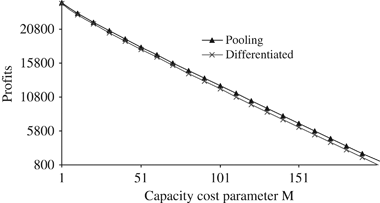
The impact of capacity cost parameter M on a firm's quotation mode decision is examined. In the numerical examples, θ=0.3 and α=0.95. M is varied from 1 to 200. The optimal Pooling UQM follows Case 1 in Table 5 and DQM follows Case 1 in Table 7. Figure 5 shows that profits from both UQM and DQM decrease when capacity parameter M increases.

Figure 5

Impact of Capacity Cost on Profits

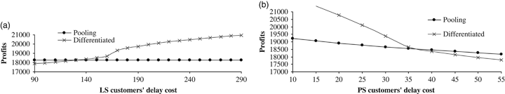
Third, the effect of the delay cost difference between LS and PS customers (β _l−β _p) on a firm's quotation mode decision is examined. In numerical examples, θ=0.3, α=0.95, and M=50. LS customers' delay cost β _l is varied from US$90/day to US$290/day in five increments. The optimal Pooling UQM follows Case 1 in Table 5 and DQM changes from Case 1 to Case 2 in Table 7. Figure 6(a) shows that the curve with “x,” providing the optimal profits from DQM, is above the profit curve of optimal pooling UQM as LS customers' delay cost increases. A firm should choose DQM when the gap between the delay costs of LS and PS customers is large. We further examine this with numerical examples where β _l is fixed at US$100/day and β _p varies from US$10/day to US$55/day. The optimal Pooling UQM follows Case 1 in Table 5 and DQM changes from Case 2 to Case 1 in Table 7. Figure 6(b) shows that the profit curve for the optimal DQM is above the curve for the pooling UQM when β _p is small, i.e., when the gap between β _l and β _p is large. Therefore, when LS and PS customers can be highly differentiated by their delay cost per unit time parameters, DQM is more attractive to a firm.

Figure 6

Impact of Delay Costs on Profits

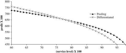
Finally, to examine the impact of service level α on a firm's quotation mode decision, θ is fixed at 0.3 while α varies from 0.6 to 0.99 in 0.01 increments. The optimal Pooling UQM follows Case 1 in Table 5 and DQM follows Case 1 in Table 7. Figure 7 has the same legend as Figure 4. The profit curves for LS Focus and PS Focus UQMs are dropped in Figure 7 because their profits are far below the profits from the pooling UQM and DQM. Profit decreases as service level α increases. This is because a firm needs to invest more in capacity to secure its lead time promise when service level increases.

Figure 7

Profit Changes with Service Level α

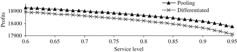
Figure 7 shows that DQM drops slightly faster than profits from UQM as service level increases. To illustrate this more clearly, we adjust the parameter values as follows: v _l=US$630, v _p=US$600, β=US$30/day, β=US$20/day, θ=0.75, and α varies from 0.6 to 0.97 in 0.01 increments. While the optimal Pooling UQM solution follows Case 1 in Table 5, the optimal DQM changes from Case 2 to Case 3 in Table 7 as α increases. Figure 8 shows that DQM becomes less attractive as service level increases. This is because the disadvantage of additional capacity cost in DQM increases when α increases.

Figure 8

DQM Becomes Less Attractive as Service Level Increases

8. Summary and Conclusions

This paper examines UQM and DQM to determine which is better for a firm and when. We provide analytical models and closed form solutions for three UQMs (LS Focus, PS Focus, and Pooling) and one DQM. By comparing profits generated from these quotation modes, we provide the following guidelines for managers to choose the right quotation mode.

When LS customers value a product or service no more than PS customers, a firm should not use DQM (Theorem 1).

If LS customers value a product or service more than PS customers, then a firm should further check the delay costs of customers. If LS customers' delay cost is just slightly larger than PS customers' delay cost, i.e., , then no DQM should be followed (Theorem 2).

Otherwise, which quotation mode is better depends on a firm's customer characteristics and operational characteristics (Theorem 3).

If PS customers have positive utilities in UQM or LS customers have positive utilities in DQM, then a firm should not use DQM (Theorem 4).

DQM may generate more revenue from customers than UQM. However, it incurs information cost and additional capacity cost. When v _l≤v _p, LS customers do not value products more than PS customers, as illustrated in section 4. LS customers are unwilling to pay more than PS customers and they are more sensitive to lead time than PS customers. So the express service option that LS customers are willing to buy also is attractive to PS customers. A firm incurs a high information cost to dissuade PS customers from choosing the express service option under DQM. In this case, the information cost cannot be justified by the extra gain from LS customers. So DQM is dominated by UQM.

When v _l>v _p and , LS and PS customers have similar delay costs. Disadvantages from information cost and from additional capacity cost under the differentiated mode are outlined. We show that information cost increases as the difference in delay cost rates β _l−β _p decreases and also increases as the difference in product valuation v _l−v _p increases. Information cost is high when customers' delay cost rates are similar. The extra profit advantage from LS customers cannot justify the information cost and the additional capacity cost incurred under DQM. So UQM again dominates DQM.

When v _l>v _p and , the information cost decreases because of increased difference between the delay cost rates of LS and PS customers. Then DQM becomes more attractive. UQM no longer always dominates DQM. Which quotation mode is better depends on parameter values. We provide detailed conditions under which DQM is better or not than UQM (Theorem 3). For this case, numerical experiments generate the following insights. When the proportion of LS customers increases, DQM is better than UQM because of increased benefits from LS customers. When the capacity cost or service level increases, DQM is less attractive to a firm because the operational disadvantage increases.

Possible extensions are as follows. First, a DQM menu can have more than two service options and customers can be classified into more than two types. Second, DQM may use shared capacity to provide differentiated services. As noted in the introduction, to implement DQM some companies use dedicated capacities while others use shared capacities. The analysis in this paper applies to dedicated capacities only. In the event that shared capacity is used, an additional constraint is introduced into the problem because maintaining the service level committment to the LS consumers may negatively affect the service level to the PS consumers. A more constrained problem will lead to a less profitable solution. Therefore, the use of DQM would then become less beneficial in comparison to UQM. On the other hand, in the event of capacity sharing, DQM no longer incurs extra capacity cost compared with UQM. Therefore, it is also possible that DQM would become more attractive in comparison to UQM. So there are advantages and disadvantages to using shared capacity for DQM. Further study is required to determine thresholds of parameters to define when DQM or UQM is best. Third, service level may become an endogenous decision variable. For example, service level shall affect customer utility and demand and thus we can modify the utility function as follows: 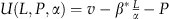. Considering α as the probability that a firm will keep its lead time promise, customers discount the lead time quotation L to be in the utility function. Following a proof very similar to the current one for Theorem 1, it can be shown that Theorem 1 remains unchanged under the new utility function. Consideration of an endogenous α value is another future research direction.

References

Abate

Choudhury

G. L.

Whitt

. 1996. Exponential approximations for tail probabilities in Queues II: Sojourn time and workload. Oper. Res. 44 (5): 758–763.

Afeche

2006. “Incentive‐compatible revenue management in queuing systems: Optimal strategic delay and other delaying tactics.” Working paper.

Afeche

Mendelson

. 2004. Pricing and priority auctions in queuing systems with a generalized delay cost structure. Manage. Sci. 50 (7): 869–882.

Ata

Olsen

T. L.

. 2009. Near‐optimal dynamic lead time quotation and scheduling under convex–concave customer delay costs. Oper. Res. 57 (3): 753–768.

Ata

Van Mieghem

. 2009. The value of dynamic resource pooling: Should a service network be integrated or product-focused? Manage. Sci. 55 (1): 115–131.

Balasubramanian

Bhardwaj

. 2004. When not all conflict is bad: Manufacturing–marketing conflict and strategic incentive design. Manage. Sci. 50 (4): 489–502.

Besanko

Donnenfeld

White

. 1987. Monopoly and quality distortion: Effects and remedies. Quart. J. Econ. 102 (4): 743–768.

Blackburn

J. D.

Elrod

Lindsley

W. B.

Zahorik

A. J.

. 1992. Manufacturing Strategy—Process and Content. Chapman and Hall, London.

Boyaci

Ray

. 2003. Product differentiation and capacity cost interaction in time and price sensitive markets. Manuf. Service Oper. Manage. 5 (1): 18–36.

10.

Dewan

Mendelson

. 1990. User delay costs and internal pricing for a service facility. Manage. Sci. 36 (12): 1502–1517.

11.

Duenyas

Hopp

W. J.

. 1995. Quoting customer lead times. Manage. Sci. 41 (1): 43–57.

12.

Easton

F. F.

Moodie

D. R.

. 1999. Pricing and lead time decisions for make‐to‐order firms with contingent orders. Eur. J. Oper. Res. 116 (2): 305–318.

13.

Fudenberg

Tirole

. 1991. Game Theory. MIT Press, Cambridge, MA.

14.

Erkoc

S. D.

Gurnani

. 2008. Delivery‐date and capacity management in a decentralized internal market. Naval Res. Logist. 55 (5): 290–405.

15.

T. H.

Zheng

. 2004. Setting customer expectation in service delivery: An integrated marketing-operations perspective. Manage. Sci. 50 (4): 479–488.

16.

Katta

Sethuraman

. 2005. “Pricing strategies and service differentiation in queues – A profit maximization perspective.” Working paper.

17.

Maglaras

Zeevi

. 2005. Pricing and design of differentiated services: Approximate analysis and structural insights. Oper. Res. 53 (2): 242–262.

18.

Mendelson

Whang

. 1990. Optimal incentive‐compatible priority pricing for the M/M/1 Queue. Oper. Res. 38 (5): 870–883.

19.

Mussa

Rosen

. 1978. Monopoly and product quality. J. Econ. Theory 18 (2): 301–317.

20.

Palaka

Erlebacher

Kropp

D. H.

. 1998. Lead time setting, capacity utilisation, and pricing decisions under lead time dependent demand. IIE Trans. 30 (2): 151–163.

21.

Pekgun

Griffin

Keskinocak

. 2008. Coordination of marketing and production for price and leadtime decisions. IIE Trans. 40 (1): 12–30.

22.

Plambeck

E. L.

2004. Optimal lead time differentiation via diffusion approximations. Oper. Res. 52 (2): 213–228.

23.

Rao

U. S.

Swaminanthan

J. M.

Zhang

. 2005. Demand and production management with uniform guaranteed lead time. Prod. Oper. Manag. 14 (4): 400–412.

24.

Ray

Jewkes

E. M.

. 2004. Customer lead time management when both demand and price are lead time sensitive. Eur. J. Oper. Res. 153 (3): 769–781.

25.

Rochet

J. C.

Chone

. 1998. Ironing, sweeping, and multidimensional screening. Econometrica 66 (4): 783–826.

26.

Rochet

J. C.

Stole

. 2003. Advances in Economics and Econometrics: Theory and Applications. Cambridge University Press, Cambridge, UK.

27.

Smith

Bailey

Brynjolfsson

. 2000. Understanding the Digital Economy. MIT Press, Cambridge, MA.

28.

K. C.

2000. Price and time competition for service delivery. Manuf. Service Oper. Manage. 2 (4): 392–409.

29.

K. C.

Song

J.‐S.

. 1998. Price, delivery time guarantees and capacity selection. Eur. J. Oper. Res. 111 (1): 28–49.

30.

Van Mieghem

J. A.

2000. Price and service discrimination in queuing systems: Incentive compatibility of Gcμ scheduling. Manage. Sci. 46 (9): 1249–1267.

31.

Webster

2002. Dynamic pricing and lead‐time policies for make‐to‐order systems. Decision Sci. 33 (4): 579–599.

Lead Time and Price Quotation Mode Selection: Uniform or Differentiated?

Abstract

Keywords

1. Introduction

2. Literature Review

2.1. Price‐Quality Screening Problem

2.2. Lead Time and Price Quotation

3. Problem Setting and Models

3.1. Models for the UQM

3.2. Model for the DQM

4. When LS Customers Value the Product No More than PS Customers

5. When v l >v p and LS Customers' Delay Cost Rate is Only Slightly Larger than PS Customers' Delay Cost Rate

5.1. DQM Under Full Information

5.2. Providing Uniform Service with Two Queues

6. When v l >v p and LS Customers have a Much Larger Delay Cost Rate than PS Customers

6.1. Optimal UQMs

6.2. Optimal Differential Quotation Modes

6.3. UQM and DQM Comparison

7. Numerical Examples

8. Summary and Conclusions

References

5. When v _l>v _p and LS Customers' Delay Cost Rate is Only Slightly Larger than PS Customers' Delay Cost Rate

6. When v _l>v _p and LS Customers have a Much Larger Delay Cost Rate than PS Customers