
Abstract
In a decentralized supply chain, supplier–buyer negotiations have a dynamic aspect that requires both players to consider the impact of their decisions on future decisions made by their counterpart. The interaction generally couples strongly the price decision of the supplier and the quantity decision of the buyer. We propose a basic model for a repeated supplier–buyer interaction, during several rounds. In each round, the supplier first quotes a price, and the buyer places an order at that price. We find conditions for existence and uniqueness of a well‐behaved subgame‐perfect equilibrium in the dynamic game. When costs are stationary and there are no holding costs, we identify some demand distributions for which these conditions are met, examine the efficiency of the equilibrium, and show that, as the number of rounds increases, the profits of the supply chain increase towards the supply chain optimum. In contrast, when costs vary over time or holding costs are present, the benefit from multi‐period interactions is reduced and after a finite number of time periods, supply chain profits stay constant even when the number of rounds increases.
Introduction
The management of supply chain relationships is an operational lever that can be critical to a firm's profitability. Indeed, supplier–buyer negotiations play a central role in establishing revenues (for suppliers) and costs (for buyers). Well‐conducted negotiations are critical in retail, for example, where giants like Wal‐Mart in the United States or Aldi in Germany strive to offer a low‐cost proposition.
The process by which a buyer and a supplier interact to fix price and sales quantity is complex. It is fraught with tensions, as the buyer is interested in obtaining a lower price and the supplier prefers a higher price provided that the sales quantity is sufficient. Generally, the outcome of such a process is not necessarily efficient for the supply chain. Indeed, prices are typically higher than the supply chain's preferred one, because the supplier requests a price strictly larger than its cost. As a result, the transacted quantities are lower than what would be best for the chain. This situation is called double marginalization, and has been documented and analyzed since the 1950s (see Spengler 1950). Much research has been done to propose supply contracts that are beneficial to buyer and supplier, such as buy‐back contracts, revenue sharing, or quantity discounts. These mechanisms allow the supply chain to move from local optimization where each company takes decisions individually, considering only its own profits, towards global optimization where the decisions of all the companies take into account aggregated supply chain profits. While these have been implemented with great success many times, they typically presuppose that the supplier or the buyer can make a take‐it‐or‐leave‐it offer, which cannot always be taken for granted. For example, two‐part tariffs (fixed fee and per‐unit fee charged by the supplier) can potentially maximize total supply chain profits, but they require that the supplier is sufficiently powerful to impose such a contract structure.
Interestingly, negotiations have a dynamic aspect that expands the strategy space of both buyer and supplier. This dynamic aspect requires both players to consider the impact of current decisions on future decisions made by their counterpart. In particular, the strategic use of inventory by the buyer has been identified as a lever to obtain lower prices from the supplier (see Anand et al. 2008). We can provide the example of the steel manufacturer Celsa, located in Spain, that procures scrap metal (the main input in steel production) from sources ranging from local scrap dealers to larger European scrap merchants. The manufacturer does not need to carry a high level of scrap metal inventory at any time, because supply is sufficiently diversified (hence no shortage is likely). However, the company stores large piles of it outside its factory. In fact, displaying such high levels of raw materials to the local dealers is an effective negotiation tool that forces them to quote lower prices. This constitutes a credible threat from the buyer: it will only buy more raw materials if the price is low enough. This example shows that a dynamic negotiation contains many interesting elements that cannot be revealed in static settings, namely, the gradual build‐up of inventory in small quantities so as to force supplier discounts.
The general analysis of such dynamic interaction between supplier and buyer is difficult. It has only been studied under simplistic settings: Most of the academic work has focused on two‐period models and/or simple linear demand functions. This is because the interaction generally couples strongly the price decision of the supplier and the quantity decision of the buyer. As a result, the analysis usually becomes intractable. In particular, it is unclear whether the outcome of the negotiation actually has a unique well‐behaved equilibrium from which supplier and buyer have no incentive to unilaterally deviate.
The purpose of this study is precisely to tackle these questions. We propose a basic model for repeated supplier–buyer interaction, during a number of rounds T. In each stage, the supplier first quotes a price, and the buyer places an order at that price. We thus focus our attention on simple wholesale price contracts, knowing that more complex contracts could coordinate the supply chain.1 The costs of delivering the order may vary over time, and the buyer may have to pay for inventory holding charges. At the end of the T rounds, the buyer faces a stochastic demand and fulfills it with its total purchase over the negotiation. With this relatively simple setting, which extends some of the existing models (Anand et al. 2008, Erhun et al. 2008), we determine how the negotiation will proceed and under which circumstances it will have a unique well‐behaved outcome. In other words, we find conditions under which we can characterize the unique subgame‐perfect equilibrium in the dynamic game. We furthermore identify some demand distributions for which these conditions are met when costs are stationary and there are no holding costs. In this scenario and for such demands, we examine the efficiency of the equilibrium and in particular show that, as T increases, the profits of the supply chain increase towards the supply chain optimum. When costs vary over time or holding costs are present, we find that the benefit from multi‐period interactions is reduced and the supply chain profits do not increase after a finite number of rounds. Our paper hence offers a technical contribution: it describes how the negotiation proceeds during multiple periods and a general demand specification.
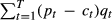
Our model reveals that the supplier will in equilibrium propose different prices in each round. At each one of these prices, the buyer will place an order. Even though prices may be decreasing in time, the buyer finds it in its best interest to place a positive order, to force the supplier to reduce its price in the following round. This results suggests that the buyer uses its cumulative purchase to reduce supplier prices in the same way as strategic inventories. Interestingly, as the length of the negotiation increases, both the supplier's and the buyer's profits increase. Indeed, this simple scheme is equivalent to using a non‐linear pricing schedule, which is able to reduce the impact of double marginalization. In other words, the effects of repeated interactions are similar to those of volume discounts, which push buyers to place larger orders by promising lower prices for the last units ordered. This insight is another contribution of the paper that echoes that of Erhun et al. (2008).
It is worth pointing out that our model extends previous work from the economics literature on price skimming (see Talluri and van Ryzin 2005 for a review), in the case where the buyer is strategic, in the context of a supply chain. Strategic customers have been studied before, but this paper considers a situation where the buyer is large enough to influence supplier pricing. That is, in our model, the buyer takes into account the impact of its purchasing decisions on future prices, in contrast with the literature (e.g., Besanko and Winston 1990). In addition, our model can be used for further extensions with many buyers and many suppliers, where buyers are not only strategic but can use their purchases to influence prices.
We start by discussing the literature relevant to this work in 2 and turn to the model in section 3. We present our results in 4 and analyze supply chain efficiency improvements in section 5. We conclude the paper in section 6 with a summary of the insights and further research. All the proofs are provided in Appendix S1.
Literature Review
This study is related to many models of supplier–buyer interactions. These models are generally included in the supply contracts literature, which focuses on aligning supply chain incentives. Cachon (2003) provides an excellent review of the field. Pasternack (1985), Cachon and Lariviere (2005), Barnes‐Schuster et al. (2002), and Eppen and Iyer (1997), among others, present supply contracts that move the supply chain toward better coordination. Our model also considers the effect of the supplier–buyer interaction on supply chain efficiency, and in particular, it shows that longer interactions (more rounds) are beneficial to both parties and the supply chain.
More specifically, the model presented here is directly related to Lariviere and Porteus (2001), where the buyer's purchased quantity and the supplier's price are analyzed in a single‐interaction setting. Song et al. (2008) examine the equilibrium price and quantity decisions for a price‐setting news vendor and in particular present the same regularity condition on the demand distribution as in Lariviere and Porteus. Van den Berg (2007) discusses the properties of the demand distribution that guarantee a well‐behaved solution to the supplier's price decision. Perakis and Roels (2007) investigate how serious double marginalization can be in a single‐period model. For this purpose, they study the worst‐case performance of supply chains, among all possible demand distributions, by considering the price of anarchy, that is, the worst‐case ratio between profits achieved by a decentralized supply chain and a centralized one. They find that the efficiency loss can be as high as 42%.
The dynamic nature of supplier–buyer interactions has also been explored before. There is work that analyzes infinitely repeated games to determine when long‐term collaborative relationships are sustainable (e.g., Debo and Sun 2004, Ren et al. 2010, Taylor and Plambeck 2007,b, Tunca and Zenios 2006, or Belavina and Girotra 2010). The general result from these studies is that when the discount rate for future profits is sufficiently high, short‐term gains from unilateral deviations prevent supply chain collaboration. In finite horizons, the study of self‐interested behavior is also quite rich. Anand et al. (2008) coin the term “strategic inventory” and show, in a two‐period setting with linear price‐dependent demand, that a buyer will find it profitable to carry inventory so as to reduce the price quoted by the supplier. Keskinocak et al. (2008) analyze a related problem with capacity constraints. Our model uncovers a similar effect. Namely, the price decision of the supplier is driven by the total purchase made by the buyer up to the date, and hence it can be used strategically by the buyer to reduce future prices. Erhun et al. (2008) is probably the work that is most similar to ours. They also analyze a multi‐period supplier–buyer interaction, with the difference that in their model the demand is deterministic and linear with price, as in Anand et al. (2008). This can be mapped in our framework to having the buyer face a uniform stochastic demand. They observe as we do that supply chain efficiency is improved as the number of rounds increases. In contrast, the focus of our work is to study the general relationship between supplier prices and buyer purchases when demand is not necessarily uniform (i.e., linear in price for Erhun et al. 2008). In particular, without linearity it is no longer guaranteed that the supplier–buyer game has a unique equilibrium. We hence focus on providing a set of conditions on the demand, for which this type of games can be analyzed. We thus prove some of the observations made in Erhun et al. (2008) that suggest that equilibrium is well behaved when the demand is Pareto or exponentially distributed when T = 2. In addition, we extend the efficiency study of Erhun et al. to uncover how it depends on the demand distribution.
Finally, some studies from the revenue management literature are also related to ours, as we study the pricing problem of the supplier. Talluri and van Ryzin (2005) provide an overview of the literature and devote one section to price skimming models, which is one of the features of our equilibrium solution. Elmaghraby and Keskinocak (2003) also review the literature: Our work falls into their replenishment/strategic‐customers category, since we have no capacity constraint, and the buyer considers its effect on the supplier's pricing strategy. With a myopic buyer, Lazear (1986) develops a model where demand is constant equal to one unit, but the buyer's valuation is uncertain and uniformly distributed. The buyer places an order as soon as the price is below its valuation. The price schedule that maximizes the expected revenue extracted by the supplier is characterized and decreases over time. Granot et al. (2011) extend Lazear's model by introducing competition between suppliers, and show that the price decrease may be exponential, rather than linear. Closer to our work is the model of Besanko and Winston (1990) that considers one supplier and many buyers. They introduce the notion of strategic customers, that is, when the buyers anticipate price decreases before placing their orders. They implicitly assume that the buyers are price‐takers, that is, their strategy has no impact on the supplier's price. In contrast, since we consider a single buyer, we take into account how the buyer's ordering strategy influences the supplier's prices.
The Model
The Setting
We consider a firm, called the buyer, that has a single opportunity to serve a stochastic demand D. We denote by f the p.d.f. of the demand, by F its c.d.f. F, and we let 
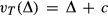
Upstream on the supply chain, a supplier sells inventory to the buyer at a price that it must choose appropriately. The details of the interaction between supplier and buyer go as follows. There are T negotiation stages, from t = 1 (first) to t = T (last, immediately before demand is realized). In each stage, the supplier proposes a price


The per‐unit cost for the supplier in period t is denoted

For the buyer, the supplier's revenue corresponds to a cost. The buyer must also take into account the cost of holding the inventory purchased: We assume that it pays a per‐unit cost of


Buyer and supplier take decisions so as to maximize their respective expected profits. We are interested in determining the subgame‐perfect equilibrium of the game that buyer and supplier play, as defined in Fudenberg and Tirole (1991). For this purpose, we consider that the strategies of each player in period t may depend on the current state of the negotiation (since we focus on subgame‐perfect equilibrium, players’ decisions can only depend on state variables that can influence the subgame from period t to T). Specifically, for each time period t, for each state of the world (this is captured through the cumulative purchase


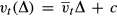
In order to understand the players’ decisions, we denote by


Similarly, we denote by


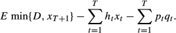
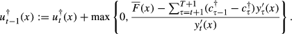
We can describe the buyer's problem in period t, given

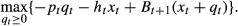
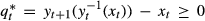
Let
 be the order that maximizes the buyer's profit at time t. Note that when


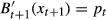

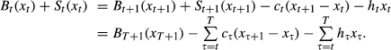
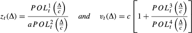
Using the optimal quantity from Equation 1, the supplier's problem can simply be expressed as 
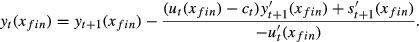
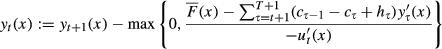
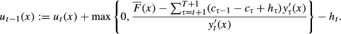
From Equation 2, we obtain
 and the corresponding
 . With this notation, we have
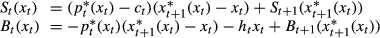
We observe that the problem's order and price paths depend only on the parameter

Note that for each negotiation stage,
Obviously, the total supply chain profit does not directly depend on the payments between buyer and supplier.
After formulating the supplier–buyer interaction, several questions arise. Given that this is a sequential game with no uncertainty during the buyer–supplier interaction, we know that a subgame‐perfect equilibrium in pure strategies exists. As in most dynamic games, it is important that this equilibrium is also unique in order for the value functions


Example and Intuition
Consider the case of a buyer that faces a stochastic demand uniformly distributed in [0,1], with no initial inventory (


In the decentralized supply chain, supplier and buyer will sequentially decide


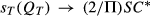
For example, when there is only one negotiation period, T = 1, the supplier would set a wholesale of p = 0.5, so that the inventory level installed by the buyer is q = 0.5. Consequently the profit of the supplier is pq = 0.25, while the expected profit of the buyer is

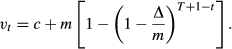
Consider now the simplest dynamic problem: the situation where there are two negotiation periods, T = 2. We can show that in equilibrium, in the first period, the supplier sets a price of


In this example, one may wonder why the buyer places an order at price


Through the example above, we can see how a longer negotiation length T can benefit both players. In the next section we develop conditions under which the buyer and supplier problems are well behaved, so that a unique equilibrium exists. Under these conditions, we can characterize the optimal supplier pricing and buyer purchasing strategies.
The T‐periods Negotiation
Existence and Uniqueness of Equilibrium
We first need to guarantee that a multi‐period equilibrium exists and is unique. It is guaranteed when the optimality problems in Equations 1 and 2 have interior unique solutions for all t = 1,…,T. This is true if and only if: for all t and for all t and
 ;
;


It is not clear that these properties are always satisfied by the recursive Equation 3. Some regularity conditions, involving the demand distribution, are hence necessary for quasi‐concavity to be preserved in the recursion. In the single‐period setting with T = 1, it has been suggested in Lariviere and Porteus (2001), Song et al. (2008), or van den Berg (2007) that it is sufficient that the demand distribution has the IGFR (increasing generalized failure rate) property, that is, that

In order to simplify the exposition, we define for each 


Let


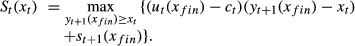
It turns out that we can rewrite in a relatively simple way


For the maximization problem to have a unique interior solution, we must have that


Using this observation in Equation 2 allows us to rewrite the equation into
This problem is well behaved when


The theorem below provides the conditions to ensure that both the buyer's and the supplier's problem have a unique optimal solution, and that both


Define When for all t = 1,…,T,
 and the buyer purchases
 .
.


The theorem characterizes recursively


More importantly, it provides a sufficient condition that guarantees that the multi‐period supplier–buyer game has a unique equilibrium. This condition is non‐trivial and has an implicit formulation. For example, when T = 1, the sufficient condition is that


Hence, for the equilibrium to be unique and well behaved, we need the demand distribution (through 


When 


It is worth pointing out an interesting property: Since


Notice that in Equations 10 and 11, the recursion depends on the shape of the demand distribution, through 

Consider If


This reformulation simplifies the analysis. Indeed, both the cost and the demand distribution have been collapsed into a single parameter, the function

Note that the demand distribution is log‐concave for uniform, exponential, gamma, or normal demands, among many others.
Furthermore, the function


Next, we solve the recursion of Equations 13 and 14 for selected demand distributions.
Consider

The lemma thus provides a closed‐form expression for


When the demand is uniformly distributed; the demand is Pareto distributed with finite mean and c = 0; the demand is exponentially distributed and c = 0. In addition, Lemma 1 can be used to establish the properties around


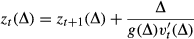
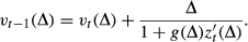
Consider g such that g(0) > 0. Then the solution to the recursive equations 13 and 14 is such that, for all t = T,…,1,
Lemma 2 hence characterizes the slope of the function


Lemma 1 is appropriate when the demand p.d.f. f is decreasing, which results in g(Δ) being an increasing function of Δ, from Equation 15. In contrast, when f is unimodal, then g(Δ) is first increasing and then decreasing in Δ. While the general analysis in that case is intractable, the following lemma identifies one family of distributions for which a closed‐form solution exists.
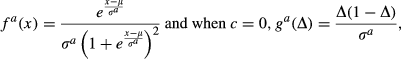
Consider g(


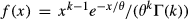
This lemma implies that for the unimodal demand distribution such that g(Δ) = aΔ(1 − (Δ/m)), a unique subgame‐perfect equilibrium in the T‐period game exists. Interestingly, this distribution can be chosen to approximate accurately a normal demand distribution. Indeed, consider a normal distribution of average μ and standard deviation σ, and c = 0. As shown in Figure 1, 
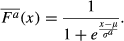


Comparison of the p.d.f. of the Normal Distribution of Mean μ = 100 and Standard Deviation σ = 30, with the p.d.f.

For this distribution,
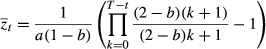
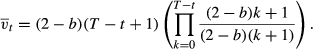
Finally, to conclude this section, we analyze in detail the solution of the recursion presented in Theorem 2 for the exponential demand. When

Consider g(


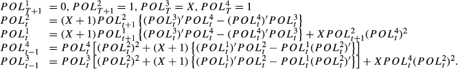
As t decreases away from T, we obtain a sequence of polynomials with positive coefficients. In addition, we find that these polynomials are such that


More generally, we numerically observe that when the demand is Gamma distributed, that is, when


Total Inventory Purchased by the Buyer as a Function of the Horizon T, for Different Values of the Cost c = 0.2,0.5,0.8 (left) and Coefficient of Variation (c.v.) of Demand


In this section, we analyze the gains of supply chain efficiency achieved by extending the length T of the negotiation. For this purpose, we compare the highest supply chain expected profit, achieved by global optimization, to the supply chain expected profit in the decentralized setting, where buyer and supplier have T negotiation periods before facing the demand. We again assume that


Asymptotic Performance with Constant Production Costs and Zero Holding Costs
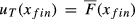
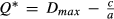
Let
 be the optimal centralized quantity that achieves global optimization:
 is such that
 . In addition, let
 be the corresponding supply chain profit. We compare
 and
and
 to
to


Consider
 .2 Then


We already knew that the longer the time horizon, the higher the buyer and the supplier's profits, because each one could always decide to purchase nothing or price sufficiently high so as to prevent sales, respectively. Both players hence benefit from a longer negotiation. This insight extends the observation made in Anand et al. (2008) that a two‐period interaction yields higher profits than the single‐period scenario. Thus, the efficiency of the supply chain improves with the number of negotiation rounds. The theorem provides a stronger statement: The joint profit asymptotically reaches the centralized supply chain profit.
This result immediately leads to another question: How fast does the ordering quantity  and
and
 ? It turns out that the convergence rate of the ordering quantity is independent of the demand distribution, as long as some regularity conditions are satisfied, as shown below in Theorem 4.


We consider first the uniform distribution in 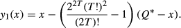
 is the centralized optimal order quantity. The total capacity installed after T negotiation stages
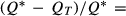
 for large T as
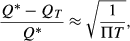
 Thus, we have
 ,
, 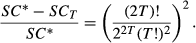


For T = 1, the supply chain inefficiency is thus 25% and for large T,
 The supply chain loss of optimality thus decreases with 1/T.
The split of profit between supplier and buyer can also be calculated. The supplier's profit can be expressed as 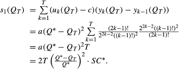
As a result, when T → ∞,
 , a result contained in Erhun et al. (2008). Also, since
 ,
,
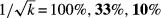
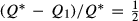
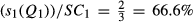
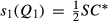 . Thus, the maximum gain achieved by the supplier is 4/Π − 1 ≈ 27.3%. The maximum supply chain gain is 4/3 − 1 = 33.3%, while the gain by the buyer is (4 − 8/Π) − 1 ≈ 45.6%. The extension of the negotiation thus benefits the buyer more than the supplier, and the supply chain share of profit for the supplier goes from
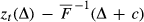
Interestingly, the asymptotic behavior of  (and Δ = 0 by using the transformation proposed in Theorem 2), the functions


Consider  and that around
 , f is smooth, that is, infinitely differentiable. Assume also that
  .3 Then, for large T,


This asymptotic result complements the observations of Erhun et al. (2008) and Anand et al. (2008). It establishes that not only does the outcome of the multi‐period negotiation improve supply chain efficiency, but also it provides a technical derivation of the speed of this improvement.
The theorem suggests that  with the square‐root of T. In addition,
 falls with
  . Finally, we observe that the sub‐optimality gap
 falls with


Theorem 4's convergence results are illustrated by the numerical experiments below. We examine the improvement of supply chain efficiency as a function of the length of the negotiation horizon. We focus on uniform, exponential, normal, and Pareto distributions. Interestingly, Perakis and Roels (2007) show that, when T = 1, the class of Pareto distributions achieves the worst‐case sub‐optimality gap. As we show below, this gap is rapidly corrected as T increases. Figure 3 (right) shows how for all four distributions plotted the sub‐optimality gap decreases with 1/T approximately. Figure 3 (left) shows the decrease of
 . Figure 4 shows how the sub‐optimality gap goes to 0 for several distributions.

Evolution of
(left) and
 (right) as a Function of T, Shown in a Log–Log Scale Plot. We Show the Results for Several Demand Distributions: the Uniform [0,1], the Exponential of Decay Rate 1, the Normal Distribution of Mean 100 and Standard Deviation 30, and the Pareto Distribution with


Optimality Gap
, for Several Demand Distributions,

Finally, we have compared the share of the supply chain profit going to the buyer. It is relatively stable, as shown in Figure 5. This implies that the additional profit generated by extending the negotiation horizon is shared approximately in a proportional manner, according to the initial split of profit with T = 1.

Share of Supply Chain Profit Going to the Buyer, for Several Demand Distributions,

The convergence results from the previous section rely on two strong assumptions. First, there are no production cost variations: As the horizon becomes longer, the total inventory purchased by the buyer gets closer to the target (the optimal quantity that maximizes supply chain profits). If the target itself increases with time, because production becomes cheaper, it may be the case that the buyer does not place orders early because they are more costly to produce for the supplier. Second, there are no inventory holding costs. If holding inventory becomes costly, then again the buyer may not find it interesting to place orders early. Both arguments suggest that any profit improvement from longer buyer–supplier interactions is limited by production cost variations and inventory holding charges. We investigate how the improvement is related to these assumptions.
In order to analyze the general case with varying


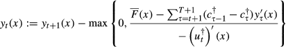
Hence,


We focus our study on the family of Gamma demand distributions, for which the regularity conditions of Theorem 1 are satisfied in all our numerical experiments. We specifically examine the impact of a fixed decrease  defined by
 , and compare the corresponding supply chain profits
  .
.


The results are depicted in Figure 6. We observe in the left part of the figure that as T increases, the ratio
 does not decrease to zero anymore and reaches a plateau after a number of rounds. That is, there is a maximum length over which the interaction between buyer and supplier is useful; if the horizon is longer than this maximum, in the initial rounds the supplier will offer a price at which the buyer places no order. This corresponds to having
  can be significant if h is high; for example even when h = 0.01 and c = 0.2, the loss is above 10% when the demand is exponential. Moreover, we observe in the right part of the figure that the maximum number of rounds during which supply chain performance can be increased is rapidly decreasing in h. Indeed, when holding costs are high, placing many small orders becomes inefficient because it requires holding inventory. Hence, if the end of the horizon is sufficiently far away, it becomes preferable not to place any order, although this implies not being able to force supplier price discounts later on.


On the Left, Evolution of
as a Function of T, for a Gamma Demand Distribution with Coefficient of Variation (c.v.)


In this study, we have presented a model to analyze repeated supplier–buyer interactions. The buyer faces a stochastic demand and must purchase inventory to serve this demand before it is realized. The inventory can be ordered from a supplier over a T‐period horizon, where in each period, the supplier chooses the price in its best interest.
We use the concept of subgame perfection to define the equilibrium price (for the supplier) and quantity purchase (for the buyer). We provide sufficient conditions to guarantee that such equilibrium is unique and well‐behaved. These conditions are satisfied for several demand distributions including uniform, approximate normal, and exponential demand. In the resulting equilibrium, the buyer will place initial orders in order to force the supplier to reduce its prices, a motivation that is similar to the use of strategic inventory in Anand et al. (2008).
In addition, we show that supply chain efficiency increases with the length of the negotiation T. Specifically, we show that when production costs do not vary and there are no holding costs, the sub‐optimality gap between the T‐periods negotiation and the centralized supply chain falls with 1/T, regardless of the demand distribution. Thus, for large T, the negotiation situation approaches the highest possible efficiency for the supply chain. When production costs vary or holding costs are positive, the sub‐optimality gap reaches a minimum for some finite T, after which it stays constant.
Interestingly, our iterative approach provides an asymptotic coordination mechanism with a single profit sharing between buyer and supplier. While it requires a more complex interaction between supplier and buyer, it replicates the effect of a quantity discounts, since the buyer now places orders at different prices with the supplier.
Furthermore, our work presents a number of interesting questions to be explored in the future. First, our work focuses on the negotiation between one supplier and one buyer, both strategic. The revenue management literature has studied in a different setting the pricing problem of one supplier pricing against one buyer with probabilistic willingness‐to‐pay. Since the supplier maximizes its expected profit, this is equivalent to pricing against infinite buyers. This situation has been studied both for myopic buyers, see Lazear (1986), and for strategic customers, see Besanko and Wilson (1990). Thus, our work considers the one‐buyer situation. The n‐buyers situation is an immediate extension of this work. Second, following Granot et al. (2011), the extension to the case of multiple suppliers is also interesting. In that situation, the buyer faces the trade‐off between placing orders in the beginning, at a higher price, so that suppliers can offer lower prices, or wait for the suppliers to compete and reduce prices. This new trade‐off may change the suppliers’ behavior in comparison with the present paper.
Footnotes
Acknowledgments
We would like to thank a senior editor and two anonymous referees for helping us improve significantly this manuscript. Victor Martínez‐de‐Albéniz's research was supported by Public‐Private Sector Research Center, IESE Business School, University of Navarra, Spain, through contract ECO 2008‐05155 of Plan Nacional del Ministerio de Ciencia y Tecnología, Spain.
1
In fact, in our model, a two‐part tariff maximizes total supply chain profits but leaves the buyer with zero profits. This is achieved by having the supplier offer extremely high prices in the first T − 1 periods and making a final take‐it‐or‐leave‐it offer in the last period.
2
From section 4.2, this is satisfied for uniform, Pareto, exponential, and an approximation of Normal.
3
From section 4.2, this is satisfied for uniform, exponential, and an approximation of Normal.