Randomization Approaches for Network Revenue Management with Customer Choice Behavior

Abstract

In this study, we present new approximation methods for the network revenue management problem with customer choice behavior. Our methods are sampling‐based and so can handle fairly general customer choice models. The starting point for our methods is a dynamic program that allows randomization. An attractive feature of this dynamic program is that the size of its action space is linear in the number of itineraries, as opposed to exponential. It turns out that this dynamic program has a structure that is similar to the dynamic program for the network revenue management problem under the so called independent demand setting. Our approximation methods exploit this similarity and build on ideas developed for the independent demand setting. We present two approximation methods. The first one is based on relaxing the flight leg capacity constraints using Lagrange multipliers, whereas the second method involves solving a perfect hindsight relaxation problem. We show that both methods yield upper bounds on the optimal expected total revenue. Computational experiments demonstrate the tractability of our methods and indicate that they can generate tighter upper bounds and higher expected revenues when compared with the standard deterministic linear program that appears in the literature.

Keywords

network revenue management customer choice dynamic programming simulation

1. Introduction

Network revenue management with customer choice behavior is well‐studied and has many applications in the airline, hotel, and car rental industries. In the context of airlines, a representative example, it involves controlling the sale of itineraries over a flight network. Customers arrive over the booking period to purchase itineraries. The airline has to decide which itineraries to make available for sale at each point in time taking into account the remaining capacities on the flight legs. This is a crucial decision to make since the customer's purchasing decision is influenced by the set of itineraries that are offered. Depending on the offer set, the customer may purchase one of the offered itineraries, or may not purchase anything and simply leave. The airline's goal is to determine the set of itineraries to offer at each point in time that maximizes the expected total revenues over the booking period. The airline's decision problem can be formulated as a dynamic program. However, computing the value functions and the optimal policy quickly become intractable and one has to resort to approximation methods.

Many of the approximation methods for the network revenue management problem with customer choice build on methods developed for network revenue management under the assumption that the customer's purchasing decision is not influenced by the set of offered itineraries. This is the so called independent demand setting, where we assume that customers arrive with the intention of purchasing a fixed itinerary. If the itinerary is available, they make the purchase. Otherwise, they leave without making any purchase. Even with the independent demand assumption, the dynamic programming formulation of the network revenue management problem becomes intractable as the size of its state space increases exponentially with the number of flight legs. Consequently, the approximation methods for the network revenue management problem with independent demand have mainly been concerned with reducing the dimensionality of the state space. Incorporating customer choice behavior adds another layer of complexity since the size of the action space also increases exponentially with the number of itineraries. This is because of the combinatorial nature of the problem of deciding which subset of itineraries to offer for sale from the set of all possible itineraries. So, while many of the approximation methods for the network revenue management problem with customer choice are able to handle the dimensionality of the state space quite well, they are less effective in dealing with the complexity of the action space. As a result, the tractability of many of the existing methods depends on the underlying model of customer choice. Much of the existing literature assumes that the customer choices are governed by the multinomial logit model and that the consideration sets, the sets of itineraries of interest to the different customer segments, are disjoint (e.g., Kunnumkal and Topaloglu 2010b, Liu and van Ryzin 2008, Zhang 2011, Zhang and Adelman 2009).

In this study, we propose new approximation methods that remain tractable for the class of random utility choice models. This class of choice models includes many of the commonly used customer choice models in the literature such as multinomial logit, nested logit, Markovian second choice, universal backup, and Lancaster demand (see Farias et al. 2013, Mahajan and van Ryzin 2001). We assume that a customer's choice decision is governed by a simple utility maximization principle. That is, a customer has a utility for purchasing each of the itineraries and to not purchasing anything. Of the available alternatives, the customer chooses the one with the highest utility. We note that this is equivalent to assuming that each customer has a ranked list of preferences and chooses the highest ranked option that is available. The starting point for our methods is a dynamic program that allows randomization. We generate a sample path of customer arrivals along with their utilities for the different itineraries and formulate a dynamic program in order to compute the optimal offer sets. We show that it is possible to reformulate this problem as a dynamic program where the number of decision variables is linear in the number of itineraries. As a result, the size of the action space becomes manageable. In fact, the resulting formulation is similar to the dynamic programming formulation of the network revenue management problem with independent demand. Consequently, we use ideas from the independent demand setting to reduce the size of the state space. We particularly focus on two approximation methods. One is based on the Lagrangian relaxation idea developed in Kunnumkal and Topaloglu (2010a) and the second is based on the randomized linear programming approach developed in Talluri and van Ryzin (1999).

The methods that we propose have a number of appealing features. Since they are sampling‐based, they can handle many of the commonly used customer choice models in the literature. In particular, we do not require the assumption that customer choices come from a multinomial logit choice model with disjoint consideration sets. Our methods yield upper bounds on the optimal expected revenue and estimates of the expected marginal values of capacity on the flight legs. The marginal value of capacity on a flight leg, referred to as its bid price, is useful in constructing control policies. On the other hand, upper bounds are useful when assessing the suboptimality of heuristic control policies. Another useful feature of our approach is that the randomized dynamic program we propose has a similar structure to the dynamic program for the network revenue management problem with independent demand. This allows us to draw upon the rich literature around the network revenue management problem with independent demand. The two approximation methods that we propose require solving only linear programs, which most commercial optimization packages are capable of. Moreover, since the linear programs we solve have only a polynomial number of variables and constraints, it minimizes the need for customized coding in the way of column generation techniques. This may enhance the practical appeal of our methods. Finally, our methods yield bid prices, which are compatible with the infrastructure of current revenue management systems that use bid price control policies.

2. Literature Review

Our work builds on previous research. Liu and van Ryzin (2008) propose a deterministic linear program for the network revenue management problem with customer choice. Zhang and Adelman (2009), Meissner and Strauss (2012b), and Zhang (2011) use the linear programming approach to approximate dynamic programming to come up with different value function approximations, where as Kunnumkal and Topaloglu (2010b) use Lagrangian relaxation ideas. All of the above mentioned methods provide upper bounds on the optimal expected revenue. However, their tractability depends on the assumptions that the customers' choices are governed by the multinomial logit model and that the consideration sets of the different customer segments are disjoint. Bront et al. (2009) analyze the case where the consideration sets overlap and show that even the column generation subproblem in the deterministic linear program of Liu and van Ryzin (2008) is NP‐hard. So even solving the deterministic linear program to get an upper bound on the optimal expected revenue becomes intractable in general.

Bront et al. (2009) and Meissner and Strauss (2011) propose heuristic methods for column generation. On the other hand, Mendez‐Diaz et al. (2011) propose a branch‐and‐cut algorithm to solve the column generation subproblem. Talluri (2011) proposes a concave program for general choice models and describes a way to randomize it. Meissner et al. (2013) build on this concave program and show how it can be strengthened by adding additional constraints. The above mentioned solution methods yield upper bounds on the optimal expected revenue as well as bid prices. There are other ways to obtain bid prices that do not necessarily yield upper bounds. Chaneton and Vulcano (2011) use stochastic approximation to compute bid prices, while Meissner and Strauss (2012a) propose a heuristic method to iteratively improve upon an initial set of bid prices.

Given a set of bid prices, they can be used in different ways to decide which set of itineraries to make available for sale at each point in time. Certain control policies involve solving a combinatorial optimization problem that has the same structure as the column generation subproblem of the deterministic linear program (e.g., Kunnumkal and Topaloglu 2010b, Zhang and Adelman 2009). As a result, they tend to be intractable in general. Other control policies tend to be easier to implement. For example, bid prices can be used in a traditional manner where an itinerary is made available for sale only if its revenue exceeds the sum of the bid prices on the flight legs that it uses (e.g., Chaneton and Vulcano 2011).

The utility maximization criterion to model customer choice behavior has appeared previously in the literature. For example, van Ryzin and Vulcano (2008) and Chaneton and Vulcano (2011) use it to model customer choice in network revenue management while Mahajan and van Ryzin (2001) use it in the context of optimizing retail assortments. The above mentioned papers assume that the random utilities (or equivalently the ranked preference lists) are available as inputs to the optimization model.

Papers concerned with estimating the parameters of the choice model include Farias et al. (2013) and van Ryzin and Vulcano (2011). Farias et al. (2013) consider a choice model where each customer is endowed with a ranked list of preferences among the products and chooses the most preferred product from the offered products. They estimate this choice model under limited data and use a robust approach to predict the revenue generated by offering a given assortment. van Ryzin and Vulcano (2011) use the Expectation‐maximization method to obtain maximum likelihood estimates of the arrival rates of customers and their ranked list of preferences.

As mentioned, our work relies on approximation methods for the network revenue management problem with independent demand. We refer the reader to Talluri and van Ryzin (2004) for a comprehensive review of the revenue management literature. The papers closest to ours are Kunnumkal and Topaloglu (2010a) and Talluri and van Ryzin (1999). Both methods yield upper bounds and bid prices for the independent demand setting. We build on these works to obtain tractable upper bounds and bid prices for the choice network revenue management problem.

In terms of choice models, the paper closest to ours is Chaneton and Vulcano (2011). Chaneton and Vulcano (2011) compute bid prices using stochastic approximation, while we use linear programming. In addition, our methods yield upper bounds on the optimal expected revenues.

Our methods involve computing expected values of functions of high dimensional random variables. As it gets intractable to obtain closed form expressions for the expected values, we resort to Monte Carlo simulation. We generate a sample of the random variables, solve optimization problems over the sample, and approximate the expected value using the sample average. Our methods thus have connections to the sample average approximation (SAA) method for solving stochastic optimization problems (e.g., Kleywegt et al. 2002).

We make the following research contributions in this study. (i) We present a new dynamic programming approximation for the network revenue management problem with customer choice behavior. This dynamic programming formulation is attractive because it allows randomization and the size of its action space is linear in the number of itineraries. (ii) We further build on this randomized dynamic program to obtain tractable approximation methods. As our methods are sampling‐based, we are not constrained by the underlying customer choice model. We are able to handle a variety of choice models; all we require is the ability to generate samples of the customers' utilities for the different alternatives. (iii) We show that our approximation methods generate upper bounds on the optimal expected revenues. Upper bounds are useful when assessing the suboptimality of heuristic control policies. We also show how our methods can be used to obtain bid prices. (iv) Computational experiments indicate that our methods can yield significantly tighter upper bounds and higher revenues than the standard deterministic linear program. Moreover, our methods are fast, easy to implement and scale well with problem size.

The rest of the article is organized as follows. Section 3 describes the network revenue management problem with customer choice behavior and formulates it as a dynamic program. In section 4, we describe the linear program proposed by Liu and van Ryzin (2008). In section 5, we present the randomized dynamic program and in section 6 we describe two tractable approximation methods based on it. The first method is based on relaxing the flight leg capacity constraints whereas the second method solves a perfect hindsight relaxation (PH). Our approximation methods are sampling‐based. We generate samples of the customers' utilities for the different alternatives and solve linear programming problems to decide on the itineraries to offer at each time period on each sample path. We use sample averages to estimate upper bounds and to obtain bid prices. Section 7 presents our computational experiments. The proofs of all the propositions and lemmas are deferred to Appendix S1 in the online Supporting Information.

3. Problem Formulation

We have an airline network consisting of a set of flight legs that we can use to serve the customers that arrive over time with the intention of purchasing itineraries. We use

L

to denote the set of flight legs in the airline network. The initial capacity on flight leg i is c _i. We use

J

to denote the set of all itineraries. An itinerary j has a revenue associated with it, which we denote by r _j. If we accept a request for itinerary j, then we consume capacity on one or more flight legs. We use a _ij to denote the number of units of capacity consumed by itinerary j on flight leg i. Naturally, we have a _ij = 0 if itinerary j does not include flight leg i. We discretize the planning horizon into a finite number of time periods

T = {1, \dots, τ}

and assume that the discretization is fine enough so that there is at most one customer arrival at each time period. The probability of a customer arrival at time period t is α. The fact that the arrival probability is constant over time is only for ease of exposition and it is straightforward to allow the arrival probability to depend on the time period t.

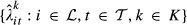
We assume that customer choice is governed by a simple utility maximization principle. That is, the customer's utilities for the different alternatives are random variables and the customer chooses the alternative with the highest utility. We note that the utility maximization principle is essentially equivalent to a choice model where customers have an ordered list of preferences and pick the most preferred alternative from the ones available. We let U _jt be the random variable which denotes the utility for purchasing itinerary j at time period t and let U _ϕt be the random variable which denotes the utility for not purchasing any itinerary at time period t. We let

U_{J} = {U_{j t} : j \in J, t \in T}

and

U_{ϕ} = {U_{ϕ t} : t \in T}

. We allow the random variables

{U_{j t} : j \in J \cup {ϕ}}

to be dependent within each time period, but assume that they are independent across time periods. In other words, the purchasing decisions of the different customers are assumed to be independent of each other. We also assume that we are able to generate samples of the random variables

{U_{j t} : j \in J \cup {ϕ}, t \in T}

. Given an offer set

S

, the customer chooses the alternative

j_{t} = {argmax}_{j \in S \cup {ϕ}} {U_{j t}}

with the highest utility. We assume that there are no ties with probability 1. The probability that the customer chooses itinerary j at time period t given the offer set

S

Pr {j_{t} = j | S} = Pr {U_{j t} = max_{k \in S \cup {ϕ}} {U_{k t}}} for j \in S .

We have

Pr {j_{t} = j | S} = 0

for

j \notin S

and the probability of purchasing nothing is

\begin{matrix} Pr {j_{t} = ϕ | S} & = Pr {U_{ϕ t} = max_{k \in S \cup {ϕ}} {U_{k t}}} \\ = 1 - \sum_{j \in J} Pr {j_{t} = j | S} . \end{matrix}

(1)

Here we emphasize that the customer's utilities for the different alternatives do not depend on the set of itineraries made available for sale. While there are choice models that do not satisfy this assumption, it covers many of the commonly used choice models in the literature (see Zhang and Cooper 2005). We also note that the purchase and no‐purchase probabilities are inputs to our model; estimating these quantities is beyond the scope of this study.

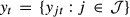
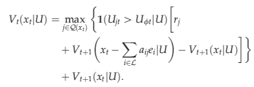
At each time period, we have to decide which itineraries to make available for sale taking into account the state of the remaining leg capacities. Using x _it to denote the remaining capacity on flight leg i at time period t,

x_{t} = {x_{i t} : i \in L}

captures the state of the remaining leg capacities. We let

Q (x_{t}) = {j \in J : a_{i j} \leq x_{i t} \forall i \in L},

(2)

denote the itineraries that can be potentially offered given the remaining leg capacities. The decision problem is to determine the set of itineraries to offer to the customers at each time period so as to maximize the expected total revenue over the planning horizon. Under the assumption that the customer arrivals in the different time periods and the purchasing decisions of the different customers are independent of each other, we can obtain the value functions

{V_{t} (\cdot) : t \in T}

through the optimality equation

\begin{matrix} V_{t} (x_{t}) & = max_{S \subset Q (x_{t})} {\sum_{j \in J} α Pr {j_{t} = j | S} [r_{j} + V_{t + 1} (x_{t} - \sum_{i \in L} a_{i j} e_{i})] \\ + [1 - α + α Pr {j_{t} = ϕ | S}] V_{t + 1} (x_{t})} \\ = max_{S \subset Q (x_{t})} {\sum_{j \in J} α Pr {j_{t} = j | S} [r_{j} + V_{t + 1} (x_{t} - \sum_{i \in L} a_{i j} e_{i}) \\ - V_{t + 1} (x_{t})]} + V_{t + 1} (x_{t}), \end{matrix}

(3)

where e _i is the

| L |

‐dimensional unit vector with a one in the element corresponding to

i \in L

and the second equality follows from Equation 1. The boundary condition for the optimality equation above is V _τ+1(·) = 0. Throughout the rest of the article, we assume that α = 1 for notational brevity. We note that this is equivalent to letting

\tilde{Pr} {j_{t} = j | S} = α Pr {j_{t} = j | S}

and

\tilde{Pr} {j_{t} = ϕ | S} = 1 - α + α Pr {j_{t} = ϕ | S}

and working with the probabilities

{\tilde{Pr} {j_{t} = j | S} : j \in J \cup {ϕ}}

Solving the above dynamic program for practical problem instances becomes difficult for two reasons. One is that the size of the state space increases exponentially with the number of flight legs in the airline network. For, if we let

C_{i} = {0, \dots, c_{i}}

, then the state space of the above dynamic program is

\prod_{i \in L} C_{i}

, which is exponential in the number of flight legs. Secondly, the size of the action space also increases exponentially with the number of itineraries in the flight network since the number of potential offer sets is of the order of

2^{| J |}

. In the following sections, we look at relaxations of problem (3) that are computationally tractable.

4. Choice‐Based Deterministic Linear Program

The choice‐based deterministic linear program (CDLP), proposed by Liu and van Ryzin (2008), is an approximation that replaces all random quantities by their expected values. If set

S

is offered at time period t, then the expected revenue obtained is

\sum_{j \in J} r_{j} Pr {j_{t} = j | S}

, while the expected capacity consumed on flight leg i is

\sum_{j \in J} a_{i j} Pr {j_{t} = j | S}

. The CDLP assumes that the revenue generated and the capacities consumed by offering set

S

take on their expected values. It determines the optimal choice of offer sets at each time period by solving

z_{C D L P} = max \sum_{t \in T} \sum_{S \subset J} \sum_{j \in J} r_{j} Pr {j_{t} = j | S} h_{t} (S)

(4)

\begin{matrix} subject to & \sum_{t \in T} \sum_{S \subset J} \sum_{j \in J} a_{i j} Pr {j_{t} = j | S} h_{t} (S) \leq c_{i} \\ \forall i \in L \end{matrix}

(5)

\sum_{S \subset J} h_{t} (S) \leq 1 \forall t \in T

(6)

h_{t} (S) \geq 0 \forall t \in T, S \subset J .

(7)

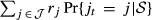
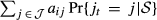
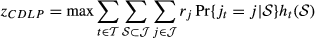
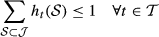
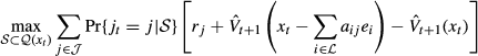
In the above linear program, the decision variable

h_{t} (S)

denotes the frequency with which set

S

is offered at time period t. The first set of constraints ensure that the expected capacity consumed on each flight leg does not exceed the available capacity. The second set of constraints ensure that the total frequency with which we offer the sets at each time period is at most one. Note that the number of decision variables in the above linear program is exponential in the number of itineraries. So in general, one has to resort to column generation to solve the problem (4)–(7). Liu and van Ryzin (2008) show that column generation can be efficiently carried out provided the choice probabilities come from the multinomial logit model and the consideration sets of the different customer segments are disjoint. Gallego et al. (2011) show that problem (4)–(7) can be reformulated as a linear program with only a polynomial number of variables provided the choice probabilities come from the multinomial logit model and the consideration sets of the different customer segments are disjoint. The column generation subproblem is hard in general; Bront et al. (2009) show that the problem is NP‐hard even for the multinomial logit choice model when the consideration sets of the different customer segments overlap.

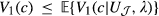
There are two main uses of CDLP. First, Liu and van Ryzin (2008) show that its optimal objective value gives an upper bound on the optimal expected total revenue. That is, we have V ₁(c) ≤ z _CDLP. Second, we can use the dual solution of the CDLP to construct heuristic control policies. Let

\hat{π} = {{\hat{π}}_{i} : i \in L}

denote the optimal values of the dual variables associated with constraints (5). Noting that

{\hat{π}}_{i}

approximates the marginal value of capacity on flight leg i, we use

{\hat{π}}_{i}

as its bid price. We can use these bid prices to come up with different control policies. Zhang and Adelman (2009) use the bid prices to obtain a value function approximation and then use this approximation in place of the value function in optimality equation 3 to decide on the offer set. That is, if

{\hat{V}}_{t} (x_{t})

is our value function approximation, we solve the problem

max_{S \subset Q (x_{t})} \sum_{j \in J} Pr {j_{t} = j | S} [r_{j} + {\hat{V}}_{t + 1} (x_{t} - \sum_{i \in L} a_{i j} e_{i}) - {\hat{V}}_{t + 1} (x_{t})]

(8)

and offer the set of itineraries which maximizes the above objective function. In the case of the CDLP, we use the value function approximation

{\hat{V}}_{t} (x_{t}) = \sum_{i \in L} {\hat{π}}_{i} x_{i t}

(9)

while solving problem (8). We note that problem (8) has a similar structure as the column generation subproblem of the CDLP. Consequently, it shares the same tractability issues. Bront et al. (2009) and Meissner and Strauss (2011) propose heuristic methods for solving problem (8). Chaneton and Vulcano (2011) use a simpler alternative: A traditional bid price control, where an itinerary is made available for sale provided its revenue exceeds the sum of the bid prices on the flight legs it uses and there is sufficient capacity.

5. Randomized Dynamic Program

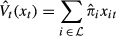
In this section, we present a randomized dynamic program for the network revenue management problem with customer choice behavior. Letting

U_{J} = {U_{j t} : j \in J, t \in T}

be a sample of the customers' utilities for the different itineraries at the different time periods, we solve the optimization problem

\begin{matrix} V_{t} (x_{t} | U_{J}) & = max_{S \subset Q (x_{t})} {\sum_{j \in J} Pr {j_{t} = j | S, U_{J}} [r_{j} \\ + V_{t + 1} (x_{t} - \sum_{i \in L} a_{i j} e_{i} | U_{J}) \\ - V_{t + 1} (x_{t} | U_{J})]} + V_{t + 1} (x_{t} | U_{J}), \end{matrix}

(10)

with the boundary condition that

V_{τ + 1} (\cdot | U_{J}) = 0

. We use the argument

U_{J}

to emphasize that the solution to the above optimality equation depends on the sampled utilities

U_{J}

and therefore is a random variable. We also note that

U_{J}

only specifies the utilities for purchasing the itineraries; the utilities for not purchasing anything

U_{ϕ} = {U_{ϕ t} : t \in T}

are still random. The following proposition shows that

E {V_{t} (x_{t} | U_{J})}

is an upper bound on V _t(x _t), where the expectation is with respect to

U_{J}

Proposition 1

We have

V_{t} (x_{t}) \leq E {V_{t} (x_{t} | U_{J})}

for all

t \in T

Note that Proposition 1 implies that

V_{1} (c) \leq E {V_{1} (c | U_{J})}

and so we get an upper bound on the optimal expected revenue by solving problem (10). Besides giving an upper bound on the value function, the randomized dynamic program also simplifies the optimization problem by reducing the size of the action space. We show below that instead of optimizing over subsets of itineraries, it is sufficient to optimize over the individual itineraries. We introduce some notation first. We let

p_{j t} (U_{J}) = Pr {j_{t} = j | {j}, U_{J}} = Pr {U_{j t} > U_{ϕ t} | U_{J}}

(11)

be the probability that the customer purchases itinerary j when it is the only itinerary that is offered at time period t. Note that the last equality follows from the fact that the customer will purchase the itinerary only if its utility exceeds the utility of not purchasing anything. We use the argument

U_{J}

to emphasize that this probability is conditional on the sampled utilities. The following lemma shows that at each time period, we can solve an optimization problem involving

| J |

decision variables as opposed to

2^{| J |}

decision variables.

Lemma 1

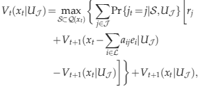
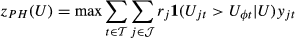
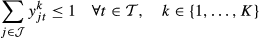
Consider the optimization problem

\begin{matrix} {\tilde{V}}_{t} (x_{t} | U_{J}) & = max {\sum_{j \in J} p_{j t} (U_{J}) y_{j t} [r_{j} \\ + {\tilde{V}}_{t + 1} (x_{t} - \sum_{i \in L} a_{i j} e_{i} | U_{J}) \\ - {\tilde{V}}_{t + 1} (x_{t} | U_{J})]} + {\tilde{V}}_{t + 1} (x_{t} | U_{J}), \end{matrix}

(12)

subject to

\sum_{j \in J} a_{i j} y_{j t} \leq x_{i t} \forall i \in L

(13)

\sum_{j \in J} y_{j t} \leq 1

(14)

y_{j t} \in {0, 1} \forall j \in J,

(15)

with the boundary condition

{\tilde{V}}_{τ + 1} (\cdot | U_{J}) = 0

. We have

V_{t} (x_{t} | U_{J}) = {\tilde{V}}_{t} (x_{t} | U_{J})

for all x _t,

t \in T

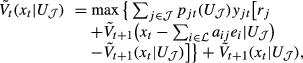
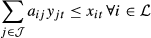
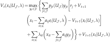
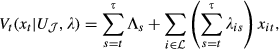
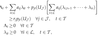
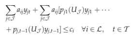
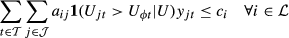
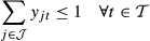
In dynamic program (12)–(15), the decision variable y _jt indicates if itinerary j is offered at time period t. More generally, we can interpret y _jt as the fraction of time itinerary j is offered at time period t. The first set of constraints ensure that the total capacity consumed on each flight leg does not exceed its available capacity. The second set of constraints ensure that we offer at most one itinerary at each time period. Although the number of decision variables in problem (12)–(15) is manageable, the size of the state space is still exponential in the capacities of the flight legs. On the other hand, noting that the decision variables in problem (12)–(15) are only over the itineraries, this problem has a similar structure to the network revenue management problem with independent demand. This allows us to use approximation ideas developed for the independent demand setting to reduce the complexity of the state space. We present two approximation methods in the following section.

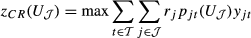
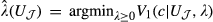
6. Relaxations of the Randomized Dynamic Program

In this section, we describe two tractable relaxations of problem (12)–(15). The first method is based on relaxing the flight leg capacity constraints using Lagrange multipliers. This yields an upper bound on the value function of the randomized dynamic program. We find the set of Lagrange multipliers which yields the tightest upper bound by solving a linear program. This idea is similar to that pursued in Kunnumkal and Topaloglu (2010a) . The second method we propose is based on solving a PH, where we have access to the customers' utilities for not purchasing anything also. This method is similar to the randomized linear programming method of Talluri and van Ryzin (1999). We note that other approximation methods developed for the network revenue management problem with independent demand can also be applied to problem (12)–(15). In this study, we particularly focus on the above‐mentioned two methods because they involve solving linear programs, which can be done quickly and efficiently. Speed is an important factor since we have to resolve the problems for many different samples.

6.1. Capacity Relaxation

Letting

Y = {y \in {0, 1}^{| J |} : \sum_{j \in J} y_{j} \leq 1}

and

y_{t} = {y_{j t} : j \in J}

, we consider relaxing constraints (13) by introducing Lagrange multipliers λ _it and solve the optimization problem

\begin{matrix} V_{t} (x_{t} | U_{J}, λ) & = max_{y_{t} \in Y} {\sum_{j \in J} p_{j t} (U_{J}) y_{j t} [r_{j} + V_{t + 1} \\ (x_{t} - \sum_{i \in L} a_{i j} e_{i} | U_{J}, λ) - V_{t + 1} (x_{t} | U_{J}, λ)] \\ + \sum_{i \in L} λ_{i t} (x_{i t} - \sum_{j \in J} a_{i j} y_{j t})} + V_{t + 1} (x_{t} | U_{J}, λ) \end{matrix}

(16)

with the boundary condition that

V_{τ + 1} (\cdot | U_{J}, λ) = 0

and

p_{j t} (U_{J})

as defined in Equation 11. The arguments

U_{J}

and λ emphasize that the solution to the above optimality equation depends on the sampled utilities for purchasing the itineraries and the Lagrange multipliers. We also note that

U_{J} = {U_{j t} : j \in J, t \in T}

does not include the utilities for not purchasing anything. The following proposition shows that as long as the Lagrange multipliers are nonnegative,

V_{t} (x_{t} | U_{J}, λ)

is an upper bound on

V_{t} (x_{t} | U_{J})

Proposition 2

λ = {λ_{i t} : i \in L, t \in T} \geq 0

, then we have

V_{t} (x_{t} | U_{J}) \leq V_{t} (x_{t} | U_{J}, λ)

Note that Propositions 1 and 2 together imply that as long as the Lagrange multipliers are nonnegative, we have

V_{1} (c) \leq E {V_{1} (c | U_{J}, λ)}

. So we are naturally interested in finding the set of Lagrange multipliers that gives the tightest upper bound. That is, for each sample

U_{J}

, we are interested in solving the problem

min_{λ \geq 0} V_{1} (c | U_{J}, λ) .

We next show that the above minimization problem reduces to solving a linear program and therefore is tractable. We begin with the following result, which gives a closed form expression for

V_{t} (x_{t} | U_{J}, λ)

Lemma 2

We have

V_{t} (x_{t} | U_{J}, λ) = \sum_{s = t}^{τ} Λ_{s} + \sum_{i \in L} (\sum_{s = t}^{τ} λ_{i s}) x_{i t},

where

Λ_{t} = {max}_{j \in J} {p_{j t} (U_{J}) [r_{j} - \sum_{i \in L} a_{i j} (\sum_{s = t + 1}^{τ} λ_{i s})] - \sum_{i \in L} a_{i j} λ_{i t}}^{+}

and we use {·}⁺ = max{0,·}.

Using the result in Lemma 2, we have that the problem

{min}_{λ \geq 0} V_{1} (c | U_{J}, λ)

can be solved as the linear program

z_{C R} (U_{J}) = min \sum_{t \in T} Λ_{t} + \sum_{i \in L} (\sum_{t \in T} λ_{i t}) c_{i}

subject to

\begin{matrix} Λ_{t} & + \sum_{i \in L} a_{i j} λ_{i t} + p_{j t} (U_{J}) [\sum_{i \in L} a_{i j} (λ_{i, t + 1} + \dots + λ_{i τ})] \\ \geq r_{j} p_{j t} (U_{J}) \forall j \in J, t \in T \\ Λ_{t} \geq 0 \forall t \in T \\ λ_{i t} \geq 0 \forall i \in L, t \in T, \end{matrix}

with the understanding that λ _i,τ+1 = 0. We use the argument

U_{J}

to indicate that the solution to the above linear program depends on the sampled utilities for purchasing the itineraries. Taking the dual of this linear program, we get

z_{C R} (U_{J}) = max \sum_{t \in T} \sum_{j \in J} r_{j} p_{j t} (U_{J}) y_{j t}

(17)

subject to

\begin{matrix} \sum_{j \in J} a_{i j} y_{j t} + \sum_{j \in J} a_{i j} [p_{j 1} (U_{J}) y_{j 1} + \dots \\ + p_{j, t - 1} (U_{J}) y_{j, t - 1}] \leq c_{i} \forall i \in L, t \in T \end{matrix}

(18)

\sum_{j \in J} y_{j t} \leq 1 \forall t \in T

(19)

y_{j t} \geq 0 \forall j \in J, t \in T,

(20)

with the understanding that y _j0 = 0. In the above linear program, we can interpret the decision variable y _jt as the frequency with which we offer itinerary j for sale at time period t. Since

p_{j t} (U_{J}) y_{j t}

represents the expected sales of itinerary j at time period t, we can interpret the first set of constraints as saying that the capacity consumed by the itineraries offered at time period t should not exceed the expected capacity consumed up to time period t, which is

c_{i} - \sum_{j \in J} a_{i j} [p_{j 1} (U_{J}) y_{j 1} + \dots + p_{j, t - 1} (U_{J}) y_{j, t - 1}]

. We emphasize that the expectations are conditional on the sampled utilities

U_{J}

. The second set of constraints ensure that the total frequency with which we offer the individual itineraries at each time period is at most one.

Letting

\hat{λ} (U_{J}) = {argmin}_{λ \geq 0} V_{1} (c | U_{J}, λ)

, we have that

E {V_{1} (c | U_{J}, \hat{λ} (U_{J}))} = E {z_{C R} (U_{J})}

is an upper bound on the optimal expected revenue. Letting

{\hat{λ}}_{i t} = E {{\hat{λ}}_{i t} (U_{J})}

, we use

\sum_{s = t}^{τ} {\hat{λ}}_{i s}

as the bid price of flight leg i at time period t. We approximate V _t(x _t) by

{\hat{V}}_{t} (x_{t}) = \sum_{i \in L} \sum_{s = t}^{τ} {\hat{λ}}_{i s} x_{i t}

(21)

and solve problem (8) using this value function approximation to decide on the set of itineraries to offer at time period t. As it becomes difficult to analytically compute the expectations

E {z_{C R} (U_{J})}

and

E {{\hat{λ}}_{i t} (U_{J})}

, we resort to Monte Carlo simulation to estimate these quantities. In particular, we generate K samples of the customers' utilities for the different itineraries

U_{J}^{1}, \dots, U_{J}^{K}

where

U_{J}^{k} = {U_{j t}^{k} : j \in J, t \in T}

are the utilities generated in the kth sample. We solve linear program (17)–(20) for each sample. Letting

z_{C R} (U_{J}^{k})

denote the optimal objective value and

{{\hat{λ}}_{i t}^{k} : i \in L, t \in T}

denote optimal values of the dual variables corresponding to constraints (18), we use

\sum_{k = 1}^{K} z_{C R} (U_{J}^{k}) / K

and

\sum_{k = 1}^{K} {\hat{λ}}_{i t}^{k} / K

as the sample estimates of

E {z_{C R} (U_{J})}

and

{\hat{λ}}_{i t} = E {{\hat{λ}}_{i t} (U_{J})}

, respectively.

6.2. Perfect Hindsight Relaxation

We consider another relaxation of problem (10) where we allow access to the customers' utilities for not purchasing anything as well. In particular, letting

U_{J} = {U_{j t} : j \in J, t \in T}

be a sample of the customers' utilities for the different itineraries at the different time periods and

U_{ϕ} = {U_{ϕ t} : t \in T}

be a sample of the customers' utilities for not purchasing anything and

U = U_{J} \cup U_{ϕ}

, we solve the optimization problem

\begin{matrix} V_{t} (x_{t} | U) & = max_{S \subset Q (x_{t})} {\sum_{j \in J} Pr {j_{t} = j | S, U} [r_{j} \\ + V_{t + 1} (x_{t} - \sum_{i \in L} a_{i j} e_{i} | U) - V_{t + 1} (x_{t} | U)]} \\ + V_{t + 1} (x_{t} | U) \end{matrix}

(22)with the boundary condition that

V_{τ + 1} (\cdot | U) = 0

. The argument U indicates that the solution to optimality equation 22 depends on the sampled utilities for all the itineraries as well as the no‐purchase alternative. Note that we can interpret problem (22) as determining the set of itineraries to offer at each time period after knowing the entire sample path: the customers' utilities for the different itineraries as well as for not purchasing anything. Proposition 3 below shows that it gives an upper bound on problem (10).

Proposition 3

We have

V_{t} (x_{t} | U_{J}) \leq E {V_{t} (x_{t} | U) | U_{J}}

for all

t \in T

Proposition 3 together with Proposition 1 imply that

V_{1} (c) \leq E {V_{1} (c | U)}

. Therefore, we obtain another upper bound on the optimal expected revenue by solving problem (22). Given the sample of the utilities U, note that

Pr {j_{t} = j | S, U} = 1 (U_{j t} > U_{ϕ t} | U)

j = {argmax}_{k \in S} {U_{k t}}

and is zero otherwise. Therefore, we have

\begin{matrix} V_{t} (x_{t} | U) & = max_{j \in Q (x_{t})} {1 (U_{j t} > U_{ϕ t} | U) [r_{j} \\ + V_{t + 1} (x_{t} - \sum_{i \in L} a_{i j} e_{i} | U) - V_{t + 1} (x_{t} | U)]} \\ + V_{t + 1} (x_{t} | U) . \end{matrix}

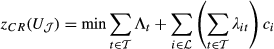
It follows that we can solve problem (22) as the following linear binary integer program:

z_{P H} (U) = max \sum_{t \in T} \sum_{j \in J} r_{j} 1 (U_{j t} > U_{ϕ t} | U) y_{j t}

(23)

subject to

\sum_{t \in T} \sum_{j \in J} a_{i j} 1 (U_{j t} > U_{ϕ t} | U) y_{j t} \leq c_{i} \forall i \in L

(24)

\sum_{j \in J} y_{j t} \leq 1 \forall t \in T

(25)

y_{j t} \in {0, 1} \forall j \in J, t \in T .

(26)

In the above problem, the decision variable y _jt indicates whether we offer itinerary j at time period t. The first set of constraints ensure that the total capacity consumed by the itinerary requests on each flight leg does not exceed its available capacity. The second set of constraints ensure that we offer at most one itinerary at each time period.

We use

E {V_{1} (c | U)} = E {z_{P H} (U)}

as an upper bound on the optimal expected revenue. In order to obtain a control policy, we solve the linear programming relaxation of problem (23)–(26). Letting

\hat{ρ} (U) = {{\hat{ρ}}_{i} (U) : i \in L}

denote the optimal values of the dual variables corresponding to constraints (24), we use

{\hat{ρ}}_{i} = E {{\hat{ρ}}_{i} (U)}

as the bid price of flight leg i. We approximate V _t(x _t) by

{\hat{V}}_{t} (x_{t}) = \sum_{i \in L} {\hat{ρ}}_{i} x_{i t}

(27)

and solve problem (8) using this value function approximation to decide on the set of itineraries to offer at time period t. It again becomes difficult to analytically compute

E {z_{P H} (U)}

and

E {{\hat{ρ}}_{i} (U)}

and so we resort to Monte Carlo simulation. In particular, we generate K samples of the customers' utilities for the different itineraries as well as not purchasing anything U ¹,…,U ^K where

U^{k} = {U_{j t}^{k} : j \in J \cup {ϕ}, t \in T}

are the utilities generated in the kth sample. We solve problem (23)–(26) for each sample. Letting z _PH(U ^k) denote the optimal objective value, we use

\sum_{k = 1}^{K} z_{P H} (U^{k}) / K

as the sample estimate of

E {z_{P H} (U)}

. Letting

{{\hat{ρ}}_{i}^{k} : i \in L}

denote the optimal values of the dual variables corresponding to constraints (24) in the linear programming relaxation of problem (23)–(26), we use

\sum_{k = 1}^{K} {\hat{ρ}}_{i}^{k} / K

as an estimate of

{\hat{ρ}}_{i} = E {{\hat{ρ}}_{i} (U)}

We close this section with a comment on the upper bounds obtained by problems (4)–(7), (17)–(20), and (23)–(26). It turns out that none of the upper bounds uniformly dominates the other. In Appendix S2 of online Supporting Information, we give examples to illustrate this. Intuitively, if there are no capacity constraints on the flight legs, then the CDLP obtains the optimal expected revenue and is therefore tighter than the other two solution methods. On the other hand, comparing the capacity relaxation (CR) and the PH, we expect the CR method to obtain a tighter bound when there is ample capacity on the flight legs and the utilities for purchasing the itineraries

U_{J} = {U_{j t} : j \in J, t \in T}

are deterministic. That is, the randomness is only in the utilities for not purchasing any itinerary. Conversely, we expect the PH method to obtain a tighter bound when there is limited capacity on the flight legs and when the utilities for not purchasing any itinerary

U_{ϕ} = {U_{ϕ t} : t \in T}

are deterministic. That is, the randomness is only in the utilities for purchasing the itineraries. Even though none of the solution methods dominates the others, in our computational experiments that we present next, we find that the CR method typically generates the tightest upper bound. The CR bound is consistently tighter than the PH bound. It is often tighter than CDLP as well.

7. Computational Experiments

In this section, we numerically compare the upper bounds and expected revenues obtained by four benchmark solution methods. We first describe the benchmark solution methods. After that we present our experimental setup and the results of the numerical study.

Choice‐based deterministic linear program (CDLP): This is the solution method that we describe in Section 4. In our practical implementation, we divide the booking horizon into five equal segments. At the beginning of each segment, we solve problem (4)–(7) after replacing the right‐hand side of Equation 5 with the remaining capacities on the flight legs and the set of time periods

T

with the current set of remaining time periods. We get a fresh set of optimal dual values

{{\hat{π}}_{i} : i \in L}

, plug them into Equation 9 and solve problem (8) to decide on the set of itineraries to offer. We continue to use this decision rule until the beginning of the next segment, where we resolve problem (4)–(7).

Capacity Relaxation (CR): This is the solution method that we describe in section 6.1. In our practical implementation, we divide the booking horizon into five equal segments. At the beginning of each segment, we solve problem (17)–(20) after replacing the right‐hand side of Equation 18 with the remaining capacities on the flight legs and the set of time periods

T

with the current set of remaining time periods. We repeat this for K samples to get a fresh set of dual values

{{\hat{λ}}_{i t}^{k} : i \in L, t \in T, k \in K}

. We use this dual values in Equation 21 to obtain our value function approximation and solve problem (8) to decide on the set of itineraries to offer. We continue to use this decision rule until the beginning of the next segment, where we resolve problem (17)–(20). We use K = 100 in our computational experiments.

Perfect hindsight relaxation (PH): This is the solution method that we describe in section 6.2. As with CDLP and CR, in our practical implementation, we divide the booking horizon into five equal segments. At the start of each segment, we refresh our bid prices by solving the linear programming relaxation of problem (23)–(26) after replacing the right‐hand side of Equation 24 with the remaining capacities on the flight legs and the set of time periods

T

with the current set of remaining time periods. We repeat this for K samples and use the fresh set of optimal dual values

{{\hat{ρ}}_{i}^{k} : i \in L, k \in K}

to obtain our value function approximation through Equation 27. We solve problem (8) to decide on the set of itineraries to offer. We continue to use this decision rule until the beginning of the next segment, where we again resolve problem (23)–(26). As in CR, we use K = 100 in our computational experiments.

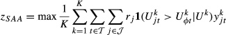
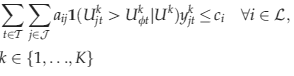
Sample average approximation (SAA): This solution method is similar to PH, but instead of solving a separate optimization problem for each sample path, we link the decisions across the different sample paths by introducing nonanticipativity constraints and solve a single optimization problem across all sample paths. SAA is based on the SAA method for stochastic programs (e.g., Kleywegt et al. 2002). The main motivation is to tighten the upper bounds obtained by, and improve the revenue performance of, PH. SAA generates K samples of the utilities {U ¹,…,U ^K} and solves

z_{S A A} = max \frac{1}{K} \sum_{k = 1}^{K} \sum_{t \in T} \sum_{j \in J} r_{j} 1 (U_{j t}^{k} > U_{ϕ t}^{k} | U^{k}) y_{j t}^{k}

(28)

subject to

\begin{matrix} \sum_{t \in T} \sum_{j \in J} a_{i j} 1 (U_{j t}^{k} > U_{ϕ t}^{k} | U^{k}) y_{j t}^{k} \leq c_{i} \forall i \in L, \\ k \in {1, \dots, K} \end{matrix}

(29)

\sum_{j \in J} y_{j t}^{k} \leq 1 \forall t \in T, k \in {1, \dots, K}

(30)

y_{j 1}^{k} = y_{j 1}^{k^{'}} \forall j \in J, k, k^{'} \in {1, \dots, K}, k \neq k^{'}

(31)

y_{j t}^{k} \in {0, 1} \forall j \in J, t \in T, k \in {1, \dots, K},

(32)

where

U^{k} = {U_{j t}^{k} : j \in J \cup {ϕ}, t \in T}

denotes the kth sample of the utilities. In the above problem, the decision variable

y_{j t}^{k}

indicates if we offer itinerary j at time period t on the kth sample path and the third set of constraints represent the nonanticipativity constraints. It is possible to show that the SAA method yields an upper bound on the optimal expected revenues and that this upper bound is tighter than that obtained by the PH method. In our practical implementation, we divide the booking horizon into five equal segments. Letting (s−1)τ/5 + 1 denote the time period marking the beginning of segment s, we solve the linear programming relaxation of problem (28)–(32) after replacing the right‐hand side of constraints (29) with the remaining capacities on the flight legs, constraints (31) with

y_{j (s - 1) τ / 5 + 1}^{k} = y_{j (s - 1) τ / 5 + 1}^{k^{'}}

, and the set of time periods

T

with the current set of time periods. Letting

{{\hat{μ}}_{i}^{k} : i \in L, k \in {1, \dots, K}}

denote the optimal dual values corresponding to constraints (29) and

{\hat{μ}}_{i} = \sum_{k = 1}^{K} {\hat{μ}}_{i}^{k}

, we show in Appendix S4 of online Supporting Information that

{{\hat{μ}}_{i} : i \in L}

is a subgradient of z _SAA with respect to the remaining leg capacities. So we use

{\hat{μ}}_{i}

as an estimate of the marginal value of capacity on flight leg i and approximate the value function V _t(x _t) by

{\hat{V}}_{t} (x_{t}) = \sum_{i \in L} {\hat{μ}}_{i} x_{i t}

. We solve problem (8) to decide on the set of itineraries to offer at time period t. We use this decision rule until the beginning of the next segment, where we resolve problem (28)–(32). We use K = 100 in our computational experiments.

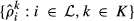
Note that the CDLP, CR, PH, and SAA control policies involve solving problem (8), which is intractable in general. In Appendix S3 of online Supporting Information, we explore simpler alternatives: We consider a traditional bid price control policy which makes an itinerary available for sale provided its revenue exceeds the sum of the bid prices on the flight legs that it uses. We also consider primal policies, which use the primal solutions to the different optimization problems to decide on the offer set. We also note that all the benchmark methods obtain bid prices that are capacity‐independent, in that they do not naturally change with the capacities on the flight legs. It is possible to obtain capacity‐dependent bid prices by using the optimal dual values obtained by the benchmark methods in a dynamic programming decomposition scheme as suggested by Liu and van Ryzin (2008) or Zhang (2011). We test the performance of the dynamic programming decomposition approaches in Appendix S3 of online Supporting Information.

We evaluate the performance of the benchmark solution methods on three groups of test problems. Customer choice is governed by the multinomial logit model in all cases. The first group involves an airline network with a single hub serving multiple spokes and is based on the test problems in Kunnumkal and Topaloglu (2010b). In these test problems, the consideration sets of the different customer segments are disjoint. The second group of test problems also involves an airline network with a single hub serving multiple spokes. However there is some level of overlap in the consideration sets of the different customer segments. The third group of test problems involves parallel flights that operate between the same origin destination pair. The consideration sets of the different customer segments overlap. These test problems are drawn from Bront et al. (2009).

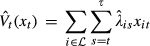
7.1. Airline Network with a Single Hub and Disjoint Consideration Sets

We consider an airline network with a single hub that serves N spokes. Half of the spokes have two flights to the hub, while the remaining half have two flights from the hub. The total number of flights is 2N. Figure 1 shows the structure of the airline network with N = 8. There are four itineraries between each spoke‐to‐hub and hub‐to‐spoke origin destination pair. On the other hand, we have eight itineraries between each spoke‐to‐spoke origin destination pair, so that the total number of itineraries is 2N(N + 2). Half of these itineraries are high fare itineraries while the other half are low fare itineraries. We let γ denote the ratio between the high fare and the low fare.

Figure 1

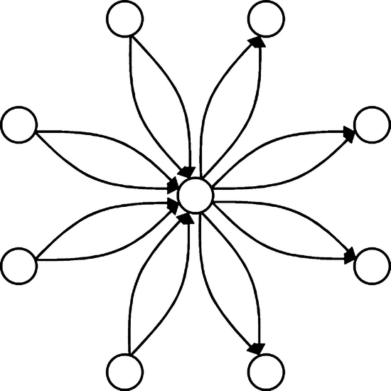
Structure of the Airline Network with a Single Hub and Eight Spokes

Each origin destination pair is associated with a customer segment. We let

K

denote the set of customer segments. At each time period a customer from segment

l \in K

arrives with probability α _l. An arriving customer is interested only in the set of itineraries connecting the origin destination pair that it is associated with. Therefore, the consideration sets of the different customer segments are disjoint. Customer choice is governed by the multinomial logit model. In the multinomial logit model, the utility for purchasing itinerary j that is in the consideration set of customer segment l is given by U _ljt = u _ljt + ξ _ljt, where u _ljt is a constant called the nominal utility and ξ _ljt is a Gumbel random variable with location parameter zero and scale parameter one. The utility for not purchasing anything for customer segment l is U _lϕt = u _lϕt + ξ _lϕt, where u _lϕt is the nominal utility for not purchasing anything and ξ _lϕt is a Gumbel random variable with location parameter zero and scale parameter one. The random variables

{ξ_{l j t} : j \in J \cup {ϕ}, t \in T}

are independent (see Ben‐Akiva and Lerman 1994).

We measure the tightness of the leg capacities in the same manner as Zhang and Adelman (2009). Letting

S_{t}^{*} = {argmax}_{S \subset J} \sum_{j \in J} r_{j} Pr {j_{t} = j | S}

be the offer set that maximizes expected revenue at time period t when there is ample capacity on all the flight legs, we use

χ = \frac{\sum_{l \in K} α_{l} \sum_{t \in T} \sum_{i \in L} \sum_{j \in J} a_{i j} Pr {j_{t} = j | S_{t}^{*}}}{\sum_{i \in L} c_{i}},

to measure the tightness of the leg capacities. We have

| T |

= 200 time periods in these test problems. We vary N, γ, and χ to obtain different test problems. We label our test problems by the triplet (N,γ,χ) ∈ {8,10,12}×{1.5,3}×{1.3,1.6}, where N is the number of spokes, γ is the ratio between the high and low fare itineraries, and χ measures the tightness, of the leg capacities. This gives us a total of 12 test problems.

Table 1 compares the upper bounds obtained by CR, PH, SAA, and CDLP. The first column in this table gives the characteristics of the problem by using (N,γ,χ). The second, third, fourth, and fifth columns, respectively, give the upper bounds obtained by CR, PH, SAA, and CDLP. The sixth column gives the percentage gap between the upper bounds obtained by PH and CR, while the last two columns give the percentage gap between the upper bounds obtained by SAA and CR, and CDLP and CR, respectively. CR performs consistently well in our computational experiments and we use CR as a benchmark. In the last three columns, a “✓ ” indicates that the gap is significant at the 95% level, while a “⊙” indicates that the gap is not significant at the 95% level. We observe that CR generates significantly tighter upper bounds than PH, SAA, and CDLP. SAA provides a small but consistent improvement over PH. On average, the upper bounds obtained by CR are about 3% tighter than PH, 2% tighter than SAA, and 9% tighter than CDLP.

Comparison of the Upper Bounds on the Optimal Expected Total Revenue for Test Problems on an Airline Network with a Single Hub and Disjoint Consideration Sets

Problem	Upper Bound				% Gap with CR
(N,γ,χ)	CR	PH	SAA	CDLP	PH	SAA	CDLP
(8, 1.5, 1.3)	2225	2448	2432	2829	9.99 ✓	9.27 ✓	27.13 ✓
(8, 1.5, 1.6)	2205	2350	2335	2646	6.57 ✓	5.87 ✓	19.99 ✓
(8, 3, 1.3)	5744	5915	5885	6469	2.99 ✓	2.47 ✓	12.63 ✓
(8, 3, 1.6)	5293	5343	5297	5502	0.95 ⊙	0.08 ⊙	3.96 ✓
(10, 1.5, 1.3)	4472	4723	4690	5082	5.60 ✓	4.86 ✓	13.62 ✓
(10, 1.5, 1.6)	4242	4357	4340	4597	2.73 ✓	2.32 ✓	8.38 ✓
(10, 3, 1.3)	10281	10414	10403	10927	1.29 ⊙	1.19 ⊙	6.28 ✓
(10, 3, 1.6)	9125	9172	9171	9243	0.51 ⊙	0.50 ⊙	1.29 ✓
(12, 1.5, 1.3)	5744	5828	5811	5996	1.45 ✓	1.16 ✓	4.38 ✓
(12, 1.5, 1.6)	5018	5052	5042	5096	0.67 ⊙	0.47 ⊙	1.55 ✓
(12, 3, 1.3)	11470	11585	11548	11992	1.01 ⊙	0.68 ⊙	4.56 ✓
(12, 3, 1.6)	10033	10087	10057	10193	0.53 ⊙	0.24 ⊙	1.59 ✓

CR, capacity relaxation; PH, perfect hindsight relaxation; SAA, sample average approximation; CDLP, choice‐based deterministic linear program.

Table 2 compares the total expected revenues obtained by CR, PH, SAA, and CDLP. We evaluate the expected revenues by simulation and use common random numbers in our simulations. The columns have a similar interpretation as in Table 1 except that they give the expected revenues obtained by the four methods. The last three columns include a “✓” if CR does better than the respective solution method at the 95% level, a “×” otherwise, and a “⊙” if there does not exist a statistically significant difference between the two. The average gap between the total expected revenues obtained by CR and CDLP is around 3%. The performance gaps are statistically significant in 10 of the 12 test problems. The performance gap between CR and CDLP seems to increase with the fare ratio and the tightness of the leg capacities. The performance gaps between CR and PH are small in most cases, although we observe one instance where PH performs about 1% better than CR. PH performs significantly better than CDLP. The average gap between the total expected revenues obtained by PH and CDLP is around 3%. The performance of SAA is comparable to that of PH in most cases.

Comparison of the Expected Total Revenues for the Test Problems on an Airline Network with a Single Hub and Disjoint Consideration Sets

Problem	Expected revenues				% Gap with CR
(N‘γ,χ)	CR	PH	SAA	CDLP	PH	SAA	CDLP
(8, 1.5, 1.3)	1975	1977	1982	1967	−0.10 ⊙	−0.35 ⊙	0.39 ⊙
(8, 1.5, 1.6)	1914	1933	1924	1918	−1.01 ×	−0.52 ×	−0.24 ⊙
(8, 3, 1.3)	5321	5336	5331	5202	−0.28 ⊙	−0.19 ⊙	2.23 ✓
(8, 3, 1.6)	4909	4930	4921	4678	−0.43 ⊙	−0.23 ⊙	4.71 ✓
(10, 1.5, 1.3)	3967	3982	3966	3908	−0.37 ⊙	0.02 ⊙	1.49 ✓
(10, 1.5, 1.6)	3821	3830	3839	3741	−0.24 ⊙	−0.46 ×	2.11 ✓
(10, 3, 1.3)	9555	9596	9564	9272	−0.43 ×	−0.10 ⊙	2.96 ✓
(10, 3, 1.6)	8711	8719	8695	8216	−0.09 ⊙	0.19 ⊙	5.68 ✓
(12, 1.5, 1.3)	5475	5457	5473	5298	0.32 ⊙	0.03 ⊙	3.23 ✓
(12, 1.5, 1.6)	4821	4793	4805	4654	0.57 ✓	0.33 ⊙	3.46 ✓
(12, 3, 1.3)	10939	10921	10924	10567	0.16 ⊙	0.14 ⊙	3.41 ✓
(12, 3, 1.6)	9640	9592	9609	9206	0.50 ✓	0.32 ⊙	4.50 ✓

CR, capacity relaxation; PH, perfect hindsight relaxation; SAA, sample average approximation; CDLP, choice‐based deterministic linear program.

Figure 2 shows how the upper bounds obtained by CR and PH change with the number of samples K for a representative test problem. We see that both CR and PH are fairly robust to the number of samples. For K ≥ 100, the widths of the confidence intervals are small enough that the differences in the upper bounds are statistically significant at the 95% level.

Figure 2

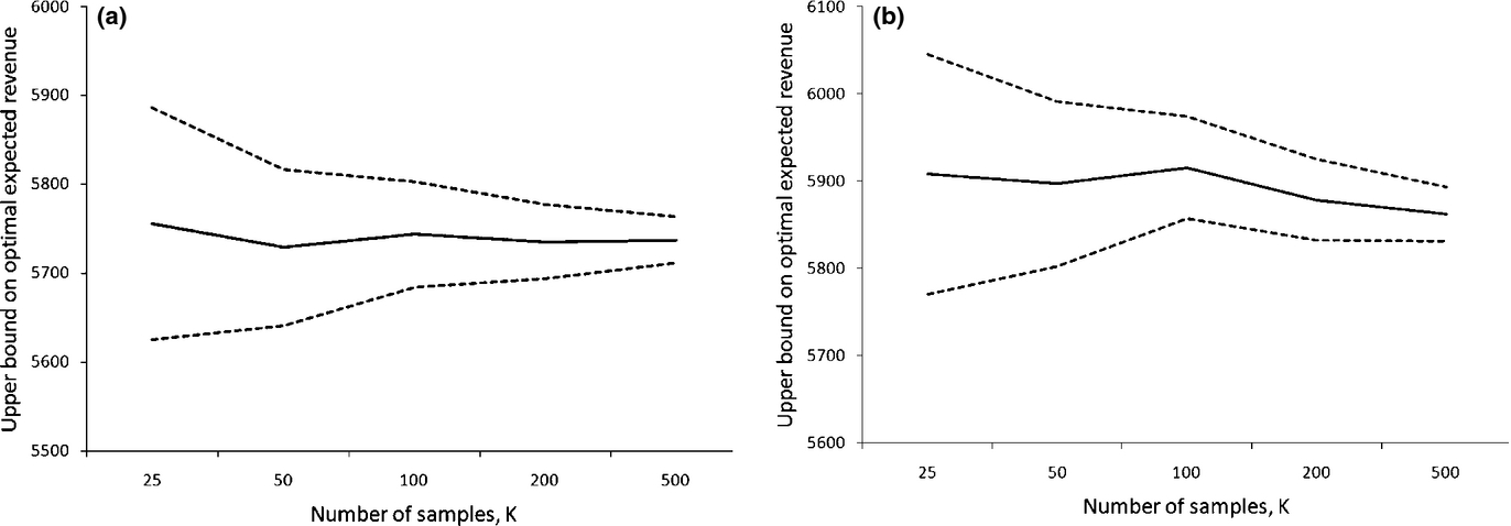
Sensitivity of the Upper Bounds Obtained by Capacity Relaxation (CR) and Perfect Hindsight Relaxation (PH) to the Number of Samples. The Plot on the Left Corresponds to CR, Whereas the Plot on the Right Corresponds to PH. The Solid line Represents the Sample Mean, While the Dashed Lines Represent the 95% Confidence Interval. The Plots are for the Test Problem on an Airline Network with a Single Hub and Disjoint Consideration Segments with Parameters (8, 3, 1.3)

Table 3 gives the CPU seconds required by the four solution methods for different numbers of spokes in the airline network and different numbers of time periods in the booking horizon. All the computational experiments are carried out on a Pentium Core 2 Duo desktop with 3‐GHz CPU and 4‐GB RAM. We use CPLEX 11.2 to solve all the linear programs. We note that since the choice probabilities come from the multinomial logit model and since the consideration sets of the different customer segments are disjoint, we do not require column generation to solve CDLP. Instead, we use the compact formulation of CDLP given in Gallego et al. (2011). The running times of PH, SAA, and CDLP are comparable and is of the order of seconds. On the other hand, the running time of CR is in minutes. We observe that the running time of PH and to some extent CR, is not very sensitive to the number of spokes in the airline network. The reason is that on each sample path, problems (23)–(26) and (17)–(20) require decision variables only for the itineraries in the consideration set of the customer segment that arrives at each time period. For example, if customer segment l _t arrives at time period t on a sample path, then we require the decision variables y _jt only for the itineraries in the consideration set of segment l _t. Since a customer segment is only interested in the set of itineraries connecting the origin destination pair that it is associated with, the sizes of the consideration sets do not increase as we increase the number of spokes in the airline network. As a result, the running times of PH and CR do not change very much.

CPU seconds for CR, PH, SAA, and CDLP as a Function of the Number of Spokes in the Airline Network and the Number of Time Periods in the Booking Horizon

	CPU seconds
	CR	PH	SAA	CDLP
No. of spokes
4	66	0.3	2	0.3
6	71	0.3	4	0.9
8	78	0.3	5	1.1
10	80	0.3	8	1.9
No. of periods
100	13	0.2	2	0.4
200	71	0.3	4	0.9
300	183	0.4	6	1.1
400	421	0.7	7	1.5

The CPU times are for an airline network with a single hub and disjoint consideration sets. For the part table under section ‘No. of spokes’, the number of time periods is 200. For the part table under section ‘No. of time periods’, the number of spokes is six.

CR, capacity relaxation; PH, perfect hindsight relaxation; SAA, sample average approximation; CDLP, choice‐based deterministic linear program.

7.2. Airline Network with a Single Hub and Overlapping Consideration Sets

We consider the same airline network as in section 7 except that each origin destination pair is now associated with two customer segments. The first segment is interested only in the low fare itineraries, while the second segment considers both the high fare and low fare itineraries connecting the origin destination pair. Within each segment, customer choice is governed by the multinomial logit model. We label our test problems by the triplet (N,γ,χ) ∈ {2,4,6}×{1.5,3}×{1.3,1.6}, which gives us a total of 12 test problems.

Table 4 compares the upper bounds obtained by the four solution methods. CR continues to obtain the tightest upper bound. The upper bound obtained by CR is on average 6% tighter than PH and SAA, and 7% tighter than CDLP. The upper bounds obtained by PH and SAA are comparable, and are about 1% tighter than CDLP on average. There are two test problems where CDLP does about 2% better than PH and SAA. However, PH and SAA obtain tighter upper bounds than CDLP in the remaining test problems and the improvements can be as high as 9%. Table 5 compares the total expected revenues obtained by the four solution methods. The results display the same trends as before. CR, PH, and SAA perform similarly on average and generate significantly higher revenues than CDLP. The average gaps between the total expected revenues obtained by CR and PH, CR and SAA, and CR and CDLP are −0.2%, −0.2%, and 3%, respectively. The tightness of the leg capacities and the size of the network as measured by the number of spokes appear to be two factors which contribute to increasing the performance gaps between CDLP and the remaining solution methods.

Comparison of the Upper Bounds on the Optimal Expected Total Revenue for the Test Problems on an Airline Network with a Single Hub and Overlapping Consideration Sets

Problem	Upper bound				% Gap with CR
(N,γ,χ)	CR	PH	SAA	CDLP	PH	SAA	CDLP
(2, 1.5, 1.3)	3405	3661	3649	3753	7.50 ✓	7.15 ✓	10.21 ✓
(2, 1.5, 1.6)	3117	3226	3222	3236	3.50 ✓	3.35 ✓	3.80 ✓
(2, 3, 1.3)	5168	5610	5594	5493	8.55 ✓	8.26 ✓	6.31 ✓
(2, 3, 1.6)	4837	5127	5118	5183	5.99 ✓	5.81 ✓	7.15 ✓
(4, 1.5, 1.3)	4621	4881	4862	5322	5.62 ✓	5.22 ✓	15.15 ✓
(4, 1.5, 1.6)	4345	4472	4461	4602	2.93 ✓	2.66 ✓	5.90 ✓
(4, 3, 1.3)	6911	7380	7360	7363	6.80 ✓	6.51 ✓	6.54 ✓
(4, 3, 1.6)	6578	6878	6861	6996	4.56 ✓	4.30 ✓	6.35 ✓
(6, 1.5, 1.3)	3290	3492	3483	3535	6.14 ✓	5.86 ✓	7.45 ✓
(6, 1.5, 1.6)	2787	2903	2900	2901	4.17 ✓	4.06 ✓	4.09 ✓
(6, 3, 1.3)	5126	5525	5513	5360	7.79 ✓	7.55 ✓	4.57 ✓
(6, 3, 1.6)	4791	5111	5103	5117	6.68 ✓	6.51 ✓	6.80 ✓

CR, capacity relaxation; PH, perfect hindsight relaxation; SAA, sample average approximation; CDLP, choice‐based deterministic linear program.

Comparison of the Expected Total Revenues for the Test Problems on an Airline Network with a Single Hub and Overlapping Consideration Sets

Problem	Expected revenues				% Gap with CR
(N,γ,χ)	CR	PH	SAA	CDLP	PH	SAA	CDLP
(2, 1.5, 1.3)	3207	3200	3203	3175	0.22 ⊙	0.13 ⊙	0.99 ✓
(2, 1.5, 1.6)	2865	2838	2833	2795	0.94 ✓	1.13 ✓	2.45 ✓
(2, 3, 1.3)	4487	4460	4441	4473	0.60 ⊙	1.03 ⊙	0.31 ⊙
(2, 3, 1.6)	4283	4214	4231	4251	1.61 ✓	1.20 ⊙	0.75 ⊙
(4, 1.5, 1.3)	4255	4276	4280	4118	−0.49 ⊙	−0.60 ×	3.20 ✓
(4, 1.5, 1.6)	3904	3903	3913	3721	0.03 ⊙	−0.22 ⊙	4.70 ✓
(4, 3, 1.3)	5743	5735	5740	5646	0.13 ⊙	0.04 ⊙	1.69 ⊙
(4, 3, 1.6)	5155	5458	5467	5184	−5.88 ×	−6.07 ×	−0.56 ⊙
(6, 1.5, 1.3)	2886	2876	2877	2730	0.33 ⊙	0.31 ⊙	5.42 ✓
(6, 1.5, 1.6)	2423	2416	2413	2281	0.29 ⊙	0.40 ⊙	5.86 ✓
(6, 3, 1.3)	4212	4217	4223	3964	−0.13 ⊙	−0.27 ⊙	5.89 ✓
(6, 3, 1.6)	4004	3994	3991	3606	0.25 ⊙	0.30 ⊙	9.93 ✓

CR, Capacity relaxation; PH, perfect hindsight relaxation; SAA, sample average approximation; CDLP, choice‐based deterministic linear program.

Table 6 gives the CPU seconds required by the four solution methods for different numbers of spokes in the airline network and different numbers of time periods in the booking horizon. Unlike the case with disjoint consideration sets, CDLP now has an exponential number of decision variables and has to be solved using column generation. The column generation subproblem can be formulated as a linear mixed‐integer program (see Bront et al. 2009). We terminate the column generation procedure when the sum of the maximum reduced profits over the time periods is within 5% of the objective value of the restricted problem (see Zhang and Adelman 2009). In contrast, the solution procedure for CR, PH, and SAA remains unchanged. As a result, the running times of CR, PH, and SAA are similar to the case with disjoint consideration sets. On the other hand, the running time of CDLP increases substantially and it can take significantly longer to solve CDLP compared to the other solution methods.

CPU Seconds for CR, PH, SAA, and CDLP as a Function of the Number of Spokes in the Airline Network and the Number of Time Periods in the Booking Horizon

	CPU seconds
	CR	PH	SAA	CDLP
No. of spokes
4	60	0.3	2	38
6	68	0.3	4	93
8	73	0.3	7	882
10	77	0.3	8	1539
No. of periods
100	9	0.2	2	59
200	68	0.3	4	93
300	135	0.4	6	153
400	323	0.5	7	276

The CPU times are for an airline network with a single hub and overlapping consideration sets. For the part table under section ‘No. of spokes’, the number of time periods is 200. For the part table under section ‘No. of time periods’, the number of spokes is six.

CR, capacity relaxation; PH, perfect hindsight relaxation; SAA, sample average approximation; CDLP, choice‐based deterministic linear program.

7.3. Parallel Flights and Overlapping Consideration Sets

We have three parallel flights that operate between the same origin destination pair. The initial capacities on the flights are 30, 50, and 40, respectively. There is a high fare and a low fare itinerary on each flight, so that the total number of itineraries is six. The revenues associated with the three low fare itineraries are 400, 500, and 300, respectively. The high fare itinerary on each flight is twice as expensive as the corresponding low fare itinerary. We have

| T | = 300

time periods in these test problems. There are four customer segments. The arrival probabilities associated with the four segments are 0.1, 0.15, 0.2, and 0.05, respectively. The first segment is only interested in the high fare itineraries, while the second customer segment is interested only in the low fare itineraries. The consideration sets of the remaining two customer segments include all the itineraries. Within each segment, choice is governed by the multinomial logit model. Letting u _j denote the nominal utility for purchasing itinerary j,

w_{j} = e^{u_{j}}

denotes the preference weight associated with itinerary j. The associated preference weights are 5, 10, and 1 for the first segment and 5, 1, and 10 for the second segment. The associated preference weights for the third and fourth segments are (10,8,6,4,3,1) and (8,10,4,6,1,3), respectively. We denote the preference weight for segment l ∈ {1,2,3,4} associated with not purchasing anything by w _lϕ. We obtain different test problems by scaling all the flight leg capacities by a factor β and varying the preference weights associated with not purchasing anything. We label our test problems by the tuple (β,(w _1ϕ,w _2ϕ,w _3ϕ,w _4ϕ)) ∈ {0.6,0.8,1.0}×{(1,5,5,1),(1,10,5,1),(5,20,10,5)}. This gives us a total of nine problems. As mentioned, these test problems are taken from Bront et al. (2009).

Table 7 compares the upper bounds obtained by CR, PH, SAA, and CDLP. The first column gives the characteristics of the problem by using

(β, (w_{1 ϕ}, w_{2 ϕ}, w_{3 ϕ}, w_{4 ϕ}))

, while the next four columns, respectively, give the upper bounds obtained by CR, PH, SAA, and CDLP. The last three columns give the percentage gap between the upper bounds obtained by PH and CR, SAA, and CR, and CDLP and CR, respectively. In these test problems, CDLP obtains the tightest upper bounds followed by CR, SAA and PH. The upper bounds obtained by CDLP are on average around 4% tighter than those obtained by CR. The gap between the bounds seems to increase with the capacities on the flight legs. This is in line with the intuition that if there were ample capacity on the flight legs, then we would expect CDLP to obtain the tightest upper bound. The average gap between the CR and SAA upper bounds is around 3%. SAA provides a small improvement on the PH upper bound.

Comparison of the Upper Bounds on the Optimal Expected Total Revenue for the Test Problems on a Parallel Flight Network and Overlapping Consideration Sets

Problem	Upper bound				% Gap with CR
(β,(w _1ϕ,w _2ϕ,w _3ϕ,w _4ϕ))	CR	PH	SAA	CDLP	PH	SAA	CDLP
(0.6,(1,5,5,1))	58632	58757	58757	56884	0.21 ⊙	0.21 ⊙	−2.98 ×
(0.6,(1,10,5,1))	58630	58757	58757	56848	0.22 ⊙	0.22 ⊙	−3.04 ×
(0.6,(5,20,10,5))	54128	55750	55697	53820	3.00 ✓	2.90 ✓	−0.57 ×
(0.8,(1,5,5,1))	74280	75465	75363	71936	1.60 ✓	1.46 ✓	−3.15 ×
(0.8,(1,10,5,1))	74264	75452	75347	71795	1.60 ✓	1.46 ✓	−3.33 ×
(0.8,(5,20,10,5))	63095	66720	66575	61868	5.74 ✓	5.52 ✓	−1.94 ×
(1.0,(1,5,5,1))	86104	87537	87386	79053	1.66 ✓	1.49 ✓	−8.19 ×
(1.0,(1,10,5,1))	84185	86560	86371	76866	2.82 ✓	2.60 ✓	−8.69 ×
(1.0,(5,20,10,5))	65645	71916	71755	63256	9.55 ✓	9.31 ✓	−3.64 ×

CR, capacity relaxation; PH, perfect hindsight relaxation; SAA, sample average approximation; CDLP, choice‐based deterministic linear program.

Table 8 compares the total expected revenues obtained by CR, PH, SAA, and CDLP. The columns have the same interpretation as in Table 7 except that they give the expected revenues obtained by the four methods. On average, CR and PH perform comparably and generate higher revenues than CDLP. The average gap between the total expected revenues obtained by CR and PH is around 0.5%, while that between CR and CDLP is around 3%. We observe two instances where SAA obtains the highest revenue among the four methods. However, on average it does not perform as well as CR and the average gap between the total expected revenues obtained by CR and SAA is around 1.5%.

Comparison of the Expected Total Revenues for the Test Problems on a Parallel Flight Network and Overlapping Consideration Sets

Problem	Expected Revenues				% Gap with CR
(β,(w _1ϕ,w _2ϕ,w _3ϕ,w _4ϕ))	CR	PH	SAA	CDLP	PH	SAA	CDLP
(0.6,(1,5,5,1))	55,320	54,368	54,422	52,986	1.72 ✓	1.62 ✓	4.22 ✓
(0.6,(1,10,5,1))	55,094	54,686	54,104	51,110	0.74 ⊙	1.80 ✓	7.23 ✓
(0.6,(5,20,10,5))	52,090	51,604	49,870	48,728	0.93 ⊙	4.26 ✓	6.45 ✓
(0.8,(1,5,5,1))	68,880	68,198	67,880	65,280	0.99 ⊙	1.45 ✓	5.23 ✓
(0.8,(1,10,5,1))	69,024	68,118	67,640	66,976	1.31 ⊙	2.01 ✓	2.97 ✓
(0.8,(5,20,10,5))	59,472	60,200	57,572	58,876	−1.22 ⊙	3.19 ✓	1.00 ⊙
(1.0,(1,5,5,1))	76,416	76,146	78,050	75,668	0.35 ⊙	−2.14 ×	0.98 ⊙
(1.0,(1,10,5,1))	74,984	74,730	76,708	72,690	0.34 ⊙	−2.30 ×	3.06 ✓
(1.0,(5,20,10,5))	61,790	62,082	59,524	60,982	−0.47 ⊙	3.67 ✓	1.31 ⊙

CR, capacity relaxation; PH, perfect hindsight relaxation; SAA, sample average approximation; CDLP, choice‐based deterministic linear program.

8. Conclusions

We presented new methods to obtain upper bounds and bid prices for the network revenue management problem with customer choice behavior. The starting point for our methods is a dynamic programming approximation that we solve for a sample of the customers' utilities for the different itineraries. An attractive feature of this randomized dynamic program is that the number of decision variables is linear in the number of itineraries. As a result, we are able to reduce the complexity of the action space. We build on this randomized dynamic program to obtain two tractable approximation methods. The first method that we propose involves relaxing the flight leg capacity constraints using Lagrange multipliers. The second method involves solving a PH. We showed that both methods give upper bounds on the optimal expected total revenue.

Our methods may also be appealing from a practical standpoint as they involve solving only linear programs. Computational experiments indicate that our methods are computationally efficient, and can significantly improve upon the upper bounds and expected revenues obtained by the CDLP. Broadly, we find that our methods are more advantageous for relatively larger test problems with tight leg capacities and large fare ratios. Problems with these characteristics typically tend to be more difficult to solve, because the consequences of offering the “wrong” set of itineraries tend to be more severe. It is therefore encouraging that the CR and PH methods provide good performance for such test problems.

Although the CR method tends to obtain tighter upper bounds than the PH method, it also tends to be more computationally intensive. On the other hand, the revenues obtained by the two methods are mostly comparable. Therefore, the CR method may be more suitable for obtaining tight upper bounds on the optimal expected total revenues, which can be done through an overnight run. On the other hand, the PH method may be more attractive to obtain control policies, where the controls need to be recomputed frequently.

One direction for future research would be to reduce the computational burden of the CR method by building on the dynamic disaggregation ideas described in Vossen and Zhang (2013). Another interesting direction would be to further strengthen the CR and PH using SAA techniques. The SAA method we presented is a first step in that direction. We find that it improves upon the upper bounds and expected revenues at a modest increase in computational time. It would be worth exploring the application of SAA ideas for multi‐stage stochastic optimization problems to the two relaxations and studying the trade‐off in solution quality with computational cost.

Footnotes

Acknowledgments

The author thanks the two anonymous referees, the senior editor, and the department editor whose comments helped substantially improve the paper. The author gratefully acknowledges the financial support of Indian School of Business.

References

Ben‐Akiva

Lerman

. 1994. Discrete Choice Analysis: Theory and Applications to Travel Demand. The MIT Press, Cambridge, MA.

Bront

J. J. M.

Mendez‐Diaz

Vulcano

. 2009. A column generation algorithm for choice‐based network revenue management. Oper. Res. 57: 769–784.

Chaneton

Vulcano

. 2011. Computing bid‐prices for revenue management under customer choice behavior. M&SOM 13(4): 452–470.

Cooper

W. L.

2002. Asymptotic behavior of an allocation policy for revenue management. Oper. Res. 50(4): 720–727.

Farias

Jagabathula

Shah

. 2013. A non‐parametric approach to modeling choice with limited data. Manage. Sci. 3(2): 305–322.

Gallego

Ratliff

Shebalov

. 2011. A general attraction model and an efficient formulation for the network revenue management problem. Working paper, Columbia University, New York.

Kleywegt

A. J.

Shapiro

Homem‐De‐Mello

. 2002. The sample average approximation method for stochastic discrete optimization. SIAM J. Optimization 12: 479–502.

Kunnumkal

Topaloglu

. 2010a. Computing time‐dependent bid prices in network revenue management problems. Transport. Sci. 44(1): 38–62.

Kunnumkal

Topaloglu

. 2010b. A new dynamic programming decomposition method for the network revenue management problem with customer choice behavior. Prod. Oper. Manag. 19(5): 575–590.

10.

Liu

van Ryzin

. 2008. On the choice‐based linear programming model for network revenue management. M&SOM 10(2): 288–310.

11.

Mahajan

van Ryzin

. 2001. Stocking retail assortments under dynamic consumer substitution. Oper. Res. 49(3): 334–351.

12.

Meissner

Strauss

A. K.

. 2011. Choice‐based network revenue management under weak market segmentation. Working paper, Department of Management Science, Lancaster University, Lancaster.

13.

Meissner

Strauss

A. K.

. 2012a. Improved bid prices for choice‐based network revenue management. Eur. J. Oper. Res. 217(2): 417–422.

14.

Meissner

Strauss

A. K.

. 2012b. Network revenue management with inventory sensitive bid prices and customer choice. Eur. J. Oper. Res. 216(2): 459–468.

15.

Meissner

Strauss

A. K.

Talluri

. 2013. An enhanced concave program relaxation for choice network revenue management. Prod. Oper. Manag. 22(1): 71–87.

16.

Mendez‐Diaz

Miranda‐Bront

Vulcano

Zabala

. 2011. A branch‐and‐cut algorithm for the latent‐class logit assortment problem. Discrete Appl. Math. (forthcoming).

17.

van Ryzin

Vulcano

. 2008. Computing virtual nesting controls for network revenue management under customer choice behavior. M&SOM 10: 448–467.

18.

van Ryzin

Vulcano

. 2011. An expectation‐maximization algorithm to estimate a general class of non‐parametric choice modelsWorking paper, New York University, New York.

19.

Talluri

2011. A randomized concave programming method for choice network revenue management. Working paper, Universitat Pompeu Fabra, Barcelona, Spain.

20.

Talluri

van Ryzin

. 1999. A randomized linear programming method for computing network bid prices. Transport. Sci. 33(2): 207–216.

21.

Talluri

van Ryzin

. 2004. The Theory and Practice of Revenue Management, Kluwer Academic Press, Norwell, MA.

22.

Vossen

Zhang

. 2013. A dynamic disaggregation approach to approximate linear programs for network revenue management Working paper, University of Colorado at Boulder, Boulder.

23.

Zhang

2011. An improved dynamic programming decomposition approach for network revenue management. M&SOM 13: 35–52.

24.

Zhang

Adelman

. 2009. An approximate dynamic programming approach to network revenue management with customer choice. Transport. Sci. 43: 381–394.

25.

Zhang

Cooper

W. L.

. 2005. Revenue management for parallel flights with customer‐choice behavior. Oper. Res., 53: 415–431.