Scalable Dynamic Bid Prices for Network Revenue Management in Continuous Time

Abstract

This study develops an approximate optimal control problem to produce time‐dependent bid prices for the airline network revenue management problem. The main contributions of our study are the analysis of time‐dependent bid prices in continuous time and the use of splines to modify the problem into an approximate second‐order cone program (ASOCP). The spline representation of bid prices permits the number of variables to depend solely on the number of resources and not on the size of the booking horizon. The advantage of this framework is the ASOCP's scalability, which we demonstrate by solving for bid prices on an industrial‐sized network. The numerical experiments highlight the ASOCP's ability to solve industrial sized problems in seconds.

Keywords

network revenue management dynamic bid prices second‐order cone programming

Introduction

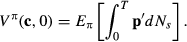
Stochastic network capacity control problems are characterized by customers arriving at random instances in time requesting products, which require different combinations of perishable resources. The most common application of network capacity control problems in revenue management (RM) is the control of reservations for airline tickets. In the airline RM problem, the single‐leg flights correspond to the perishable resources and the available origin–destination (OD) itineraries comprise the set of products. Airlines can maximize their revenue by determining whether or not to accept an itinerary request. Given sufficient resources, the optimal policy for an airline is to accept a booking request for an itinerary if its fare is greater than the opportunity cost of required resources. The opportunity cost of each flight depends on the number of available seats in the network and the remaining time in each flight's booking horizon. Although the optimal controls can theoretically be found using the Bellman equation, even for a modest sized airline network the problem suffers from the curse of dimensionality.

The intractability of the airline RM problem has lead to an extensive literature proposing various heuristics and approximate solutions. One fundamental approach is to derive bid prices, which approximate the value of each resource, using a deterministic linear program (LP). The resulting control policy is to sell the itinerary if its fare is greater than the sum of the bid prices of seats on flights in the requested itinerary. The shortcoming of the bid price policy based on the LP is that the bid prices are static over the booking horizon. Thus, the bid prices do not adjust as the system evolves until the LP is re‐optimized using the updated capacity levels.

Adelman (2007) proposed an alternative bid price approach, the dynamic linear program (DLP), by modeling the revenue function with an affine approximation to obtain time‐dependent bid prices. Adelman derived the DLP directly from the Bellman's equation, developed appropriate bounds on the performance of the method, demonstrated structural properties, and proposed a solution approach based on column generation. However, approximating the revenue function and generating time‐dependent bid prices remain difficult for large networks due to the number of variables and constraints in the DLP problem. Network models that generate dynamic (time or capacity dependent) bid prices have become an active area of RM research, since Adelman's seminal paper. Research on dynamic bid prices extends existing formulations to incorporate other aspects of RM or provides novel computational approaches to improve performance.

Topaloglu (2009) decomposed itinerary request decision by flight leg using Lagrangian relaxation to create capacity‐dependent bid prices. Kunnumkal and Topaloglu (2010) subsequently extended this model by also incorporating time‐dependence into the inventory‐sensitive bid prices. Extensions of existing models include Zhang and Adelman (2009), who integrated Liu and van Ryzin's customer choice based LP into Adelman's initial model and Kunnumkal and Topaloglu (2008), who incorporated customer choice behavior into their Lagrangian relaxation time‐sensitive bid prices model. Meissner and Strauss (2012) formulated an inventory‐sensitive bid price model with customer choice and demonstrated that their model encapsulates the choice based LPs by Zhang and Adelman (2009), Kunnumkal and Topaloglu (2008), and Liu and Van Ryzin (2008). Since we focus strictly on time‐dependent bid prices, the phrases “dynamic bid prices” and “time‐dependent bid prices” are used interchangeably throughout this study.

Both Tong and Topaloglu (2014) and Vossen and Zhang (2015) present new methods for producing time‐dependent bid prices, recognizing that the number of variables and constraints as well as the column generation procedure prevent the DLP from being implemented in practice. Tong and Topaloglu (2014) showed that the column generation problem for the dual to Adelman's DLP can be solved in polynomial time by using a minimum cost network flow problem. Using the network flow structure, they were able to reduce the number of constraints from exponential to linear in the number of flight legs. Vossen and Zhang (2015) use a Dantzig–Wolfe reformulation to provide the same reduction found in Tong and Topaloglu (2014). Vossen and Zhang (2015) also develop a novel dynamic disaggregation algorithm to solve the reduced programs, utilizing the fact that bid prices only change toward the end of the booking horizon.

Although network RM problems are traditionally modeled based on discrete time, in reality, customer arrivals occur in continuous time. As Bitran and Caldentey (2003) point out in their overview of RM and pricing, continuous time models of RM problems are more appropriate than their discrete counterparts given the growth of e‐commerce and the Internet. Bitran and Caldentey's observation could not be more relevant for network RM in the current business environment as exemplified by travel websites such as Expedia, Priceline, Travelocity, and Orbitz which attract over 7.5 millions people each day.

While continuous time formulations are used extensively in dynamic pricing research, only Akan and Ata (2009) have used a continuous time framework to obtain and study bid prices in the network RM setting. Akan and Ata highlight that the nonoptimality of classical bid‐price controls stems from discreteness and implement a generalized bid price control, which combines bid‐prices with a capacity usage limit process to determine how much of the demand rate to accept. Using a nonnegative stochastic process to characterize bid prices, they demonstrated that the optimal generalized bid price process forms a martingale. While Akan and Ata's model is not readily applicable for solving large‐scale problems, their model is general and provides several important theoretical insights into the structure of bid prices. Rather than representing the bid prices as stochastic processes, our model (like Adelman) utilizes an affine functional form to approximate the value function and develop bid prices. Working in continuous time diminishes the impact of time on the number of variables and the number of constraints, which helps address the shortcomings of previous approaches regarding the problem size. The challenge with the continuous time formulation is replacing the infinite collection of constraints with a finite set and selecting a finite‐dimensional family of functions to approximate the bid prices. Applying properties from the optimality conditions of the problem, we construct a scalable computational procedure by representing the derivatives of the bid price functions with cubic splines and reformulating the problem as a second‐order cone program. The cubic splines allow the number of the bid price variables to be independent of the size of the booking horizon making it scalable to larger networks.

Our numerical experiments demonstrate that the revenue benefits from discrete time dynamic bid prices dissipate in a continuous time setting as the problem scale increases. In comparison, by developing an approach from continuous time, our method is able to maintain revenue improvements over an LP bid price policy that is updated several thousands of times as the network size increases. By implementing our method on the Porter Airlines network, which consists of 182 flight legs, 2196 products, and 70 seats on each flight, we establish that our continuous time formulation can generate effective time‐dependent bid prices on an industrial scale.

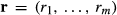
The remainder of the study is organized as follows. In section 2, we introduce notation, formally define the network RM problem, and present the Hamilton–Jacobi–Bellman (HJB) conditions, which serves as a starting point for our model. In section 3, we derive our bid price approach directly from the optimal control problem of the network RM problem by introducing two approximations into the problem. The first approximation introduces approximation of the value function using time‐dependent bid prices and the second reduces the number of variables and constraints in the problem by an implicit treatment of the accept/reject controls. We establish the optimality conditions and structural properties for the approximate optimal control problem in section 4. In section 5, we use the established properties to select a finite‐dimensional family of functions of time that can approximate the derivatives of bid prices and reduce the infinite collection of constraints to a finite set. The resulting model is an approximate second‐order cone program (ASOCP). Three sets of numerical experiments illustrating our model's effectiveness are presented in section 6. The first two sets of experiments compare discrete and continuous dynamic bid prices against LP bid prices over a randomly generated network in continuous time. The third set of experiments computes bid prices from our solution method over the Porter Airlines network to demonstrate the potential of our method's performance in an industrial setting. Finally, in section 7 we provide a brief summary and directions for future research. Please see Appendix S1 for proofs.

Network Revenue Management Problem in Continuous Time

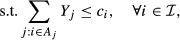
The capacity control approach to network RM can be described as follows. Consider a firm which has m perishable resources with capacities

c_{i}

i \in I \equiv {1, \dots, m}

which expire at time T. The firm uses these resources to offer n products during the time interval [0, T]. The price of each product

j \in J \equiv {1, \dots, n}

is fixed at

p_{j}

, and demands for the products are described by a collection of independent (possibly nonhomogeneous) Poisson processes with continuous intensities

λ_{j, t}

. One unit of demand for product

j \in J

requires

a_{i, j}

units of resource

i \in I

. We assume that the entries of

A = ‖ a_{i, j} ‖

are 0 or 1 and that of

c = {(c_{1}, \dots, c_{m})}^{'}

are positive integers. In this case, column

A_{j}

of A is an incidence vector of resources required by product j. The described capacity and demand structure is a common assumption in RM models for such applications as airline and hotel RM.

In particular, it is still a common practice among airlines to fix prices

p = {(p_{1}, \dots, p_{n})}^{'}

and only control whether a particular product is offered at a given time within the selling horizon. Thus, the capacity control process

u_{j, t}

j \in J

at time t, specifies whether to accept (

u_{j, t} = 1

) or reject (

u_{j, t} = 0

) an incoming demand request for product j. Let

N_{t} = {(N_{1, t}, \dots, N_{n, t})}^{'}

be a vector of Poisson processes with intensities

(u_{1, t} λ_{1, t}, \dots, u_{n, t} λ_{n, t})

modulated by the controls. Let

U

be the class of all nonanticipating control processes

u_{t} = {(u_{1, t}, \dots, u_{n, t})}^{'}

which satisfy

\int_{0}^{T} A d N_{t} \leq c (a.s.)

(1)

and

u_{j, t} \in {0, 1}

j \in J

, t ∈ [0, T]. The expected total revenue of policy

π \in U

V^{π} (c, 0) = E_{π} [\int_{0}^{T} p^{'} d N_{s}] .

The capacity control problem is to find a policy

π^{*}

which attains

V^{*} (c, 0) = {sup}_{π \in U} V^{π} (c, 0)

. The optimal policy for this intensity control problem is of Markovian form and Theorem VII.1 of Bremaud (1981) provides sufficient HJB conditions. Let

r = (r_{1}, \dots, r_{m})

be the vector of remaining capacities, and

r_{t} = c - A N_{t}

be the remaining capacity process. Constraints 1 are equivalent to the condition that

A u_{t} \leq r_{t}

holds almost surely. Let

U (r) = {u \in {0, 1}^{n} : A u \leq r}

, and

V^{*} (r, t)

be the value function, that is, the optimal expected total revenue given capacities r at time t ≤ T. Then the HJB conditions are given by the following differential equations

\frac{\partial}{\partial t} V^{*} (r, t) + \max_{u \in U (r)} {\sum_{j \in J} λ_{j, t} u_{j} [p_{j} - (V^{*} (r, t) - V^{*} (r - A_{j}, t))]} = 0,

(2)

for all t ∈ [0, T] and

r \in R = {r \in Z_{+}^{m} : r \leq c}

, with the boundary conditions

V^{*} (r, T) = 0, \forall r \in R, and

(3)

V^{*} (0, t) = 0, \forall t \in [0, T] .

(4)

We observe that the maximum in Equation 2 gives the optimal controls of the threshold form

u_{j}^{*} (r, t) = \{\begin{matrix} 1, if p_{j} \geq V^{*} (r, t) - V^{*} (r - A_{j}, t), \\ 0, otherwise . \end{matrix}

(5)

The policy implies that given sufficient resources it is optimal to fulfill the demand request as long as the revenue received from this request is greater than the opportunity cost of the required resources in terms of the expected revenues from future sales. On substituting optimal controls Equations 5 into 2, we get differential equations of the form

\frac{\partial}{\partial t} V^{*} (r, t) + \sum_{j \in J : A_{j} \leq r} λ_{j, t} max {p_{j} - (V^{*} (r, t) - V^{*} (r - A_{j}, t)), 0} = 0 .

(6)

This a system of ordinary differential equations for

V^{*} (\cdot, t)

(treated as an

| R |

‐dimensional vector) with continuous dependence on t and Lipschitz‐continuous on

V^{*} (\cdot, t)

. A known result from the theory of differential equations (see Corollary 2.4.5 of Vinter 2000) implies that there exists a unique solution, in the Sobolev space

W^{1, 1} [0, T]

. The functions in this space are almost everywhere differentiable on [0, T], Lebesgue integrable along with their derivatives (belong to

L^{1} [0, T]

), and equal to the integrals of their derivatives (absolutely continuous). The norm in

W^{1, 1} [0, T]

is the sum of

L^{1} [0, T]

norms (the integral of the absolute value) of the function and its derivative. Unfortunately, the exact solution of Equation 6 cannot be computed in most practical problems because of the extremely high number of dimensions of

V^{*} (\cdot, t)

. In the next section, we discuss approximations to

V^{*} (r, t)

which can be obtained with reasonable computational effort.

Approximate Optimal Control Problem

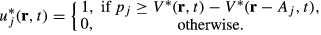
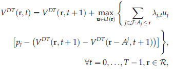
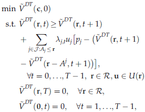
We start by contrasting our approach to approximating the network capacity control problem with that of Adelman (2007), who starts with a discrete time version of the problem where it is assumed that the time unit is sufficiently small for

\sum_{j \in J} λ_{j, t} \leq 1

to hold and for the intensities

λ_{j, t}

to be interpreted as probabilities of booking request arrivals in period t. A discrete time analog of Equation 2 is

\begin{matrix} V^{D T} (r, t) = V^{D T} (r, t + 1) + \max_{u \in U (r)} {\sum_{j \in J : A_{j} \leq r} λ_{j, t} u_{j} \\ [p_{j} - (V^{D T} (r, t + 1) - V^{D T} (r - A^{j}, t + 1))]}, \\ \forall t = 0, \dots, T - 1, r \in R, \end{matrix}

with the boundary conditions of the same form as Equations (3)–(4). The discrete time HJB conditions can be equivalently restated as a LP of the form

\begin{matrix} min {\tilde{V}}^{D T} (c, 0) \\ s.t. {\tilde{V}}^{D T} (r, t) \geq {\tilde{V}}^{D T} (r, t + 1) \\ + \sum_{j \in J : A_{j} \leq r} λ_{j, t} u_{j} [p_{j} - ({\tilde{V}}^{D T} (r, t + 1) \\ - {\tilde{V}}^{D T} (r - A^{j}, t + 1))], \\ \forall t = 0, \dots, T - 1, r \in R, u \in U (r) \\ {\tilde{V}}^{D T} (r, T) = 0, \forall r \in R, \\ {\tilde{V}}^{D T} (0, t) = 0, \forall t = 1, \dots, T - 1, \end{matrix}

where

{\tilde{V}}^{D T} (r, t)

's are the variables. This LP is still intractable for instances of realistic size because of the extremely large number of variables. Therefore, Adelman (2007) restricts the values of these variables to a subspace represented by a linear combination of a certain collection of basis functions. A particularly tractable case is provided by the linear function of the capacity vector

{\tilde{V}}^{D T} (r, t) = v_{0, t} + \sum_{i \in I} v_{i, t} r_{i}

. The values

v_{i, t}

have an appealing interpretation of the dynamic bid prices. A dynamic control policy resulting from this representation reduces to accepting a booking request if and only if its fare

p_{j}

is greater or equal to the sum of bid prices of the required resources

\sum_{i \in A_{j}} v_{i, t}

at the time t of the request arrival. With a slight abuse of notation,

i \in A_{j}

represents all resources used by product j.

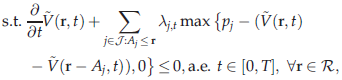
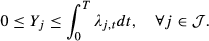
Our approach differs from that of Adelman (2007) by the use of continuous time methods in approximating the value function as well as the use of a different starting point – Equation 6 rather than Equation 2. Consider a variational problem of the form

min \tilde{V} (c, 0)

(7)

\begin{matrix} s.t. \frac{\partial}{\partial t} \tilde{V} (r, t) + \sum_{j \in J : A_{j} \leq r} λ_{j, t} max {p_{j} - (\tilde{V} (r, t) \\ - \tilde{V} (r - A_{j}, t)), 0} \leq 0, a.e. t \in [0, T], \forall r \in R, \end{matrix}

(8)

\tilde{V} (r, T) = 0, \forall r \in R,

(9)

and trajectories

\tilde{V} (\cdot, t)

in the space

W^{1, 1} [0, T]

, where “a.e.” stands for “almost everywhere” in the Lebesgue measure. Constraint 8 is a differential inequality that limits the derivatives of

\tilde{V} (\cdot, t)

from above. Constraints (8)–(9) used with r = 0 imply that

\tilde{V} (0, t) \geq 0

for all t ∈ [0,T]. This removes the need to explicitly impose the equivalent of boundary condition 4 in the variational problem. Intuitively, the value of

\tilde{V} (c, 0)

is the smallest when all inequalities are satisfied as equalities. As the result, the optimal value of

\tilde{V} (c, 0)

is equal to

V^{*} (c, 0)

. The proof of the following formal statement is straightforward:

Lemma 1

V^{*} (\cdot, t)

is the optimal solution to Equation (7)–(9).

The idea of the proof is to observe that

V^{*} (\cdot, 0)

is a feasible trajectory for Equation (7)–(9), and any feasible solution to Equation (7)– (9)has a property

\tilde{V} (r, t) \geq V^{*} (r, t)

for all

r \in R

and t ∈ [0, T].

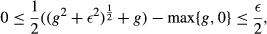
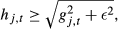
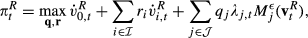
We now consider a restriction of the Problem (7)–(9), where:

The feasible trajectories are restricted to a subspace represented as

\tilde{V} (r, t) = v_{0, t} + \sum_{i \in I} v_{i, t} r_{i} .

The max operator is approximated from above by the following lemma (the proof is immediate):

Lemma 2

For any g,

\frac{1}{2} ({(g^{2} + ϵ^{2})}^{\frac{1}{2}} + g) \to max {g, 0}

from above uniformly as ε→0. Moreover,

0 \leq \frac{1}{2} ({(g^{2} + ϵ^{2})}^{\frac{1}{2}} + g) - max {g, 0} \leq \frac{ϵ}{2},

where the upper bound is attained for g = 0.

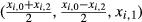
Constraint 8 uses terms of the form

max {g_{j, t}, 0}

where

g_{j, t} = p_{j} - (\tilde{V} (r, t) - \tilde{V} (r - A_{j}, t)) = p_{j} - \sum_{i \in A_{j}} v_{i, t},

represents a profit estimate from product j based on the bid prices at time t. We replace

max {g_{j, t}, 0}

with the expression

M_{j}^{ϵ} (v_{t}) = \frac{1}{2} {([p_{j} - \sum_{i \in A_{j}} v_{i, t}]^{2} + ϵ^{2})^{\frac{1}{2}} + p_{j} - \sum_{i \in A_{j}} v_{i, t}},

which approximates it from above within

\frac{ϵ}{2}

. The resulting approximate optimal control problem (AOCP) is

min v_{0, 0} + \sum_{i \in I} v_{i, 0} c_{i},

(10)

s.t. {\dot{v}}_{0, t} + \sum_{i \in I} r_{i} {\dot{v}}_{i, t} + \sum_{j \in J : A_{j} \leq r} λ_{j, t} M_{j}^{ϵ} (v_{t}) \leq 0, a.e. t \in [0, T], \forall r \in R,

(11)

v_{i, T} = 0, \forall i \in I \cup {0} .

(12)

Since AOCP results from restricting the feasible set of the Problem (7)–(9), we conclude the following:

Lemma 3

The optimal value of AOCP is an upper bound for

V^{*} (c, 0)

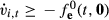
Although AOCP belongs to the general class of control problems for unbounded differential inclusions, we are able to derive rather simple optimality conditions for it using results of Loewen and Rockafellar (1994). The inclusion is unbounded since

{\dot{v}}_{i, t}

on a feasible state trajectory can be arbitrarily low.

Optimality Conditions for AOCP

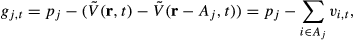
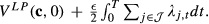
For convenience, we let the function of t,

v_{t}

and

{\dot{v}}_{t}

representing the left‐hand‐side of 11 be denoted as

f_{r} (t, v_{t}, {\dot{v}}_{t})

and its last term, which does not depend on

{\dot{v}}_{t}

, as

f_{r}^{0} (t, v_{t})

. Because of its additive structure,

f_{r}^{0} (t, v_{t})

can be expressed as

f_{r}^{0} (t, v_{t}) = \sum_{j \in J : A_{j} \leq r} λ_{j, t} M_{j}^{ϵ} (v_{t})

. We use this representation to make the statement of the optimality conditions more compact:

Theorem 1

v_{t}^{*} = (v_{i, t}^{*}, i \in I \cup {0})

is an optimal bid price trajectory for the problem (10)–(12), then there exist an adjoint trajectory

z_{t} = (z_{i, t}, i \in I \cup {0})

and multipliers

μ_{r, t} \geq 0

r \in R

for almost all t such that the adjoint differential inclusion (the Euler–Lagrange inclusion) holds for almost all t:

{\dot{z}}_{0, t} = 0,

(13)

{\dot{z}}_{i, t} = \sum_{r \in R} μ_{r, t} \sum_{j : A_{j} \leq r, i \in A_{j}} λ_{j, t} \frac{\partial M_{j}^{ϵ}}{\partial v_{i, t}} (v_{t}^{*}), i \in I,

(14)

z_{0, t} = \sum_{r \in R} μ_{r, t},

(15)

z_{i, t} = \sum_{r \in R} μ_{r, t} r_{i}, i \in I,

(16)

μ_{r, t} = 0, r \notin B_{t},

(17)

where

B_{t} = {r \in R : f_{r} (t, v_{t}^{*}, {\dot{v}}_{t}^{*}) = 0}

is the set of active constraints in 11; the Weierstrass‐Pontryagin maximum condition holds for almost all t:

\sum_{i \in I \cup {0}} z_{i, t} {\dot{v}}_{i, t}^{*} = max \sum_{i \in I \cup {0}} z_{i, t} w_{i},

(18)

s.t. w_{0} + \sum_{i \in I} r_{i} w_{i} + f_{r}^{0} (t, v_{t}^{*}) \leq 0, r \in R;

(19)

and the transversality condition holds

z_{0, 0} = 1,

(20)

z_{i, 0} = c_{i}, i \in I .

(21)

Moreover, collection

{μ_{r, t}, r \in R}

is an optimal solution to the dual of the LP problem in (18)–(19).

The optimality conditions of Theorem 1 are essential for further analysis of the optimal solution to AOCP. In particular, we obtain the following monotonic property:

Corollary 1

The adjoint trajectory has the following properties:

z_{0, t}

is constant and equals 1, that is,

z_{0, t} = \sum_{r \in R} μ_{r, t} = 1,

and

{\dot{z}}_{i, t} \leq 0

i \in I

for almost all t with a strict inequality unless

z_{i, t} = 0

The second property asserted in Corollary 1 means that

z_{i, t}

i \in I

is strictly decreasing unless it is zero. This corollary also suggests an interpretation to the adjoint variables

z_{i, t}

and multipliers

μ_{r, t}

. Since

μ_{r, t}

are nonnegative and add to 1 they can be interpreted as probability distribution over all possible capacity vectors. Strictly positive

μ_{r, t}

's identify active constraints, and their values represent relative contributions of the corresponding constraints to the optimal objective value. Value of

z_{i, t}

is the expected value of the ith component of the capacity vector over this distribution. Additional insights are revealed from the form of adjoint Equation 14. From the proof of Corollary 1, we see that the value of

- \frac{\partial M_{j}^{ϵ}}{\partial v_{i, t}} (v_{t})

is zero for

i \notin A_{j}

, identical for

i \in A_{j}

and belongs to the interval [0, 1]. Moreover, it approximates an indicator function of the event that the revenue from product j exceeds the sum of bid prices of resources in

A_{j}

. Since the latter is the acceptance rule for demand requests, the negative of the inner summation in Equation 14 approximates the intensity of utilization of resource i when capacities are given by r. Therefore,

{\dot{z}}_{i, t}

decreases approximately at the rate of expected intensity of resource i utilization where the expectation is with respect to probability mass

μ_{r, t}

. According to a general control‐theoretic interpretation, adjoint variables play the role of shadow prices by measuring the impact on the value function of a unit change in the state variables on the optimal trajectory of the system. Applying this general interpretation to our problem, we conclude that

z_{i, t}

measures, on the optimal bid‐price trajectory, the impact of a unit change in bid price

v_{i, t}

on the value of the upper bound. Corollary 1 and 14 imply that this impact is strictly decreasing at the expected rate of resource utilization until it reaches zero and stays constant after that. The second result is a monotonicity property of the bid prices:

Corollary 2

The optimal bid price trajectory of AOCP is decreasing and nonnegative in every component

v_{i, t}^{*}

i \in I \cup {0}

. Moreover, bid price

v_{i, t}

i \in I

remains constant from time 0 until

t_{i}^{'}

such that

z_{i, t_{i}^{'}} = 1

In addition to the managerial implication that dynamic bid prices produced by the continuous time model decrease over time, this result reveals that each bid price remains constant for some period of time starting from the beginning of the planning horizon. The length of these intervals is determined from the adjoint variables. Corollary 2 also suggests a way to eliminate a bulk of constraints from the problem. Consider any decreasing bid price trajectory

v_{t}

. Observe that

f_{r + e_{i}}^{0} (t, v_{t}) = f_{r^{'}}^{0} (t, v_{t})

whenever the set of depleted resources in r and

r^{'}

is the same. If

r^{'} \geq r

we have

f_{r + e_{i}} (t, v_{t}, {\dot{v}}_{t}) \geq f_{r^{'}} (t, v_{t}, {\dot{v}}_{t})

because

{\dot{v}}_{t} \leq 0

and

{\dot{v}}_{t}

enters into these functions with nonnegative coefficients. This immediately implies the following

Corollary 3

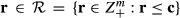
If we modify the Problem 10–12 by adding a constraint that all state components

v_{i, t}

i \in I \cup {0}

are decreasing and removing all constraints in 11 corresponding to r which have some component greater than 1, then the resulting problem has the same optimal solution as 10–12.

The resulting reduced set of constraints is indexed by the set

\bar{R} = {r \in R : r_{i} \leq 1, i \in I}

. We refer to the modified AOCP problem where a feasible bid price trajectory is constrained to be monotone and the constraint index set

R

is replaced by

\bar{R}

as AOCPM.

Corollaries 1–3 parallel findings in Adelman (2007). The interpretation of

μ_{r, t}

from Corollary 1 as a probability distribution is analogous to the interpretation of the dual variables in the DLP as state action probabilities. The monotonicity property of the time‐dependent bid prices from Corollary 2 was established for DLP in Theorem 2 of Adelman (2007). One advantage of the continuous time formulation that transpires in Corollary 2 is a relatively easy‐to‐prove property of constant bid prices at the beginning of the planning horizon. The motivation for adding the monotonicity constraints in Corollary 3 stems from Adelman's numerical experiments, which demonstrated that these additional constraints vastly improve the solution speed of the problem. In addition, Adelman proves that the objective value of the DLP is bounded from above by the static LP. We show that AOCP has a similar property up to an additive term which is proportional to the accuracy ε of approximation for the max operator. The static LP is a problem which maximizes the total expected revenues from all products subject to the constraints that the expected sales are less than the expected demand, and that the network has sufficient capacity. If

Y_{j}

is the expected number of seats sold for product j then the static LP is

V^{L P} (c, 0) = \max_{Y} \sum_{j} p_{j} Y_{j},

(22)

s.t. \sum_{j : i \in A_{j}} Y_{j} \leq c_{i}, \forall i \in I,

(23)

0 \leq Y_{j} \leq \int_{0}^{T} λ_{j, t} d t, \forall j \in J .

(24)

The following proposition is established by constructing a feasible solution to the static LP problem 22–24 from an optimal solution to AOCP.

Proposition 1

An optimal solution to AOCP yields a feasible solution to the standard LP and its value is bounded from above by

V^{L P} (c, 0) + \frac{ϵ}{2} \int_{0}^{T} \sum_{j \in J} λ_{j, t} d t .

The proposition shows that the bound on

V^{*} (c, 0)

becomes no worse than

V^{L P} (c, 0)

as ε goes to zero. From the proof, it is also evident that the actual bound provided by AOCP may be even better. However, the main advantage of AOCP is not in the bound it provides but in the continuous time computational approaches to finding dynamic bid prices.

Remark 1

The theorems and lemmas presented in this section assume the existence of an optimal solution to AOCP. Augmenting AOCP with a lower bound constraint on

{\dot{v}}_{i, t}

i \in I \cup 0

places it into a general class of the optimal control problems P discussed in subsection 2.6 of Vinter (2000). Proposition 2.6.2 in Vinter (2000) states that P has a minimizer. With the additional bound on

{\dot{v}}_{i, t}

i \in I \cup 0

, all assumptions of Proposition 2.6.2 Vinter are satisfied and consequently, there exists an optimal solution. For this bounded AOCP, the Euler–Lagrange inclusion is similar to that of Theorem 1 except Equations 15 and 16 become respectively:

\begin{matrix} z_{0, t} = \sum_{r \in R} μ_{r, t} - ξ_{0, t} \\ z_{i, t} = \sum_{r \in R} μ_{r, t} r_{i} - ξ_{i, t}, i \in I, \end{matrix}

where

ξ_{i, t} \geq 0

play the role of Lagrange multipliers for the boundary constraints. The modified optimality conditions can be used to establish structural results for the bounded AOCP. The choice of the lower bound on

{\dot{v}}_{i, t}

should not a priori exclude any vertices of the constraint set 19. One such option is

{\dot{v}}_{i, t} \geq - f_{e}^{0} (t, 0)

(where e is the m‐dimensional vector of ones). No vertex is excluded because

f_{e}^{0} (t, 0) \geq f_{r}^{0} (t, v)

for any v ≥ 0,

r \in R

Finite‐Dimensional Computational Strategies for AOCP

In this section, we discuss finite‐dimensional computational strategies for solving AOCP. There are several key points that need to be taken into account. First, we need to select an appropriate family of functions of time that can approximate feasible state trajectories

v_{t}

, t ∈ [0, T] of the AOCP. This family must be described by a finite number of parameters. Second, we need to devise a constraint generation strategy that permits us to replace an infinite collection of constraints in differential inclusion Equation 11 with a finite set. The two points are related, because the continuity and differentiability properties of functions in the family may affect the number of constraints that have to be explicitly considered. The nature of relation follows from constraints 11 that involve both the bid price trajectory and its derivative. Indeed, if a bid price trajectory satisfies constraints 11 only for a given finite number of time points, then the continuity of the trajectory and its derivative permits us to reduce constraint violations for other time points. The proposed computational strategy addresses both of these points and leads to a finite‐dimensional LP with second‐order cone constraints.

Reduction to a Finite‐Dimensional Problem

Bid‐price trajectories

v_{t}

, t ∈ [0, T] of the AOCP belong to the normed space

W^{1, 1} [0, T]

of a.e. differentiable functions. Since constraints of AOCP involve both

v_{t}

and its derivative

{\dot{v}}_{t}

, we need to develop a computationally tractable representation for either object. It is sufficient to start with the derivative. Indeed, if

{\dot{v}}_{t}

is approximated in terms of

L_{1}

‐norm within a sufficiently small tolerance by an integrable function

{\dot{v}}_{t}^{A}

, then

v_{t}

is approximated by

v_{t}^{A} = - \int_{t}^{T} {\dot{v}}_{t}^{A} d t

within a small tolerance in the stronger pointwise sense (

L_{\infty}

‐norm). The objective function for the approximate problem is:

v_{0, 0}^{A} + \sum_{i \in I} v_{i, 0}^{A} c_{i} .

(25)

We recall that any function in

L_{1} [0, T]

can be approximated by a twice continuously differentiable function (see, e.g., Theorem 2.16 from Lieb and Loss 2001 claiming a stronger result about approximation by infinitely differentiable functions). Within the class of such functions, we focus on the cubic splines:

{\dot{v}}_{i, t}^{A} = - \sum_{l = 0}^{3} a_{i, l}^{k} {(\frac{t - t_{k}}{t_{k + 1} - t_{k}})}^{l}, \forall t \in [t_{k}, t_{k + 1}],

(26)

where

t_{k}

k \in K \equiv {1, \dots, K}

is a collection of appropriate knot points and

a_{i, l}^{k},

l \in L \equiv {0, \dots, 3}

are the coefficients of the spline on the interval

[t_{k}, t_{k + 1})

for resource

i \in I

. Continuity of this approximation and its derivatives is ensured by the constraints:

\begin{matrix}  \end{matrix} a_{i, 0}^{k + 1} = \sum_{l = 0}^{3} a_{i, l}^{k},

(27)

\frac{1}{t_{k + 2} - t_{k + 1}} a_{i, 1}^{k + 1} = \sum_{l = 1}^{3} \frac{l}{t_{k + 1} - t_{k}} a_{i, l}^{k},

(28)

\frac{2}{{(t_{k + 2} - t_{k + 1})}^{2}} a_{i, 2}^{k + 1} = \sum_{l = 2}^{3} \frac{l (l - 1)}{{(t_{k + 1} - t_{k})}^{2}} a_{i, l}^{k},

(29)

that apply to every k ∈ {1,…,K − 1} and

i \in I

. The value of

v_{i, t}^{A}

is found as the integral of Equation 26 on the interval [t,T]

v_{i, t}^{A} = - \int_{t}^{T} {\dot{v}}_{i, t}^{A} d t,

(30)

which is a linear expression of the variables

a_{i, l}^{k}

k \in K

l \in L

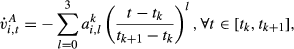
Since we already know that AOCP is equivalent to AOCPM, it makes sense to restrict

{\dot{v}}_{i, t}^{A}

to be nonpositive or, equivalently, the cubic spline represented by

a_{i, l}^{k}

's to be nonnegative. To enforce nonnegativity of the cubic splines, we use a method that was recently employed by Alizadeh et al. (2008) in the context of statistical estimation of arrival rates. Applying the characterization of nonnegative functions in Tchebysheff systems (see Karlin and Studden 1966) to cubic splines over a finite set, Alizadeh et al. enforce nonnegativity using semidefinite matrices. For each spline component index

k \in K

and

i \in I

, we use Theorem 1 of Alizadeh et al. (2008) claiming that the necessary and sufficient conditions for nonnegativity of cubic polynomial

Σ_{l = 0}^{3} a_{i, l}^{k} {(\frac{t - t_{k}}{t_{k + 1} - t_{k}})}^{l}

are provided by the following representation of the coefficients:

a_{i, 0}^{k} = y_{i, 0}^{k},

(31)

a_{i, 1}^{k} = 2 y_{i, 1}^{k} + x_{i, 0}^{k} - y_{i, 0}^{k},

(32)

a_{i, 2}^{k} = y_{i, 2}^{k} + 2 x_{i, 1}^{k} - 2 y_{i, 1}^{k},

(33)

a_{i, 3}^{k} = x_{i, 2}^{k} - y_{i, 2}^{k},

(34)

\frac{x_{i, 0}^{k} + x_{i, 2}^{k}}{2} \geq \sqrt{{(\frac{x_{i, 0}^{k} - x_{i, 2}^{k}}{2})}^{2} + {(x_{i, 1}^{k})}^{2}},

(35)

\frac{y_{i, 0}^{k} + y_{i, 2}^{k}}{2} \geq \sqrt{{(\frac{y_{i, 0}^{k} - y_{i, 2}^{k}}{2})}^{2} + {(y_{i, 1}^{k})}^{2}} .

(36)

Constraints (35)–(36) are equivalent to restricting matrices

X_{i}^{k} = (\begin{matrix} x_{i, 0}^{k} x_{i, 1}^{k} \\ x_{i, 1}^{k} x_{i, 2}^{k} \end{matrix})

and

Y_{i}^{k} = (\begin{matrix} y_{i, 0}^{k} y_{i, 1}^{k} \\ y_{i, 1}^{k} y_{i, 2}^{k} \end{matrix})

to being positive semidefinite. This type of constraint is well studied in the area of optimization known as semidefinite programming (SDP). Together, Constraints (27)–(36) enforce monotonicity of bid prices.

In a practical implementation, variables

a_{i, l}^{k}

can be eliminated by substituting representation Equations (31)–(34) into 26 and 30. In fact, for each

i \in I \cup 0

and time interval

[t_{k}, t_{k + 1}]

only six variables are needed to represent dynamic bid price

v_{i, t}^{A}

. The number of variables is effectively independent of time and depends on the number of resources and knot points. Moreover, after the substitution, the monotonicity of bid price

v_{i, t}^{A}

on the entire interval

[t_{k}, t_{k + 1}]

is enforced by just two constraints (35)–(36). Given that the proposed approximation of the derivative

{\dot{v}}_{t}^{A}

requires a finite number of variables and the objective of AOCPM is linear, our problem reduces to a semi‐infinite optimization problem (SIP). There are several standard approaches for solving SIP (see López and Still 2007 for a recent review). Here, we construct a finite problem by restricting constraint collection Equation 11 to a set of grid‐points

T \subset [0, T]

. In Appendix S2, we utilize results from Still (2001) to bound the approximation error from limiting the SIP to a set

T

consisting of

N_{k}

evenly spaced grid‐points over

[t_{k}, t_{k + 1}]

k \in K

. The error bound can be used to check the approximation accuracy after solving for the spline coefficients through the ASOCP. In the subsequent development, we assume that

T

contains the set of spline knot points

t_{k}

k \in K

and

t_{K + 1} = T

We complete the construction of the approximate problem by observing that constraints 11 restricted to

t \in T

can be converted to a second‐order conic constraints by introducing variables

g_{j, t}

and

h_{j, t}

j \in J

t \in T

such that

h_{j, t} \geq \sqrt{g_{j, t}^{2} + ϵ^{2}},

(37)

g_{j, t} = p_{j} - \sum_{i \in A_{j}} v_{i, t}^{A} .

(38)

Constraints 35, 36, and 37 equivalently require that the vectors

(\frac{x_{i, 0} + x_{i, 2}}{2}, \frac{x_{i, 0} - x_{i, 2}}{2}, x_{i, 1})

(\frac{y_{i, 0} + y_{i, 2}}{2}, \frac{y_{i, 0} - y_{i, 2}}{2}, y_{i, 1})

, and

(h_{j, t}, g_{j, t}, ϵ)

belong to the three‐dimensional second‐order (Lorentz) cone. Each constraint of the form Equation 11 is replaced by

{\dot{v}}_{0, t}^{A} + \sum_{i \in I} r_{i} {\dot{v}}_{i, t}^{A} + \sum_{j \in J : A_{j} \leq r} λ_{j, t} \frac{1}{2} (h_{j, t} + g_{j, t}) \leq 0,

(39)

for each

t \in T

and

r \in \bar{R}

. The maximum slack (equivalently, the minimum violation) in this constraint is obtained when

h_{j, t}

is as small as possible, forcing the equality in Equation 37.

The resulting approximate SOCP problem (ASOCP) is to minimize the linear objective Equation 25 with respect to the variables

X_{i}^{k}

Y_{i}^{k}

a_{i, l}^{k}

{\dot{v}}_{i, t}^{A}

v_{i, t}^{A}

g_{j, t}

, and

h_{j, t}

where the indices range over the sets

i \in I \cup {0}

j \in J

t \in T

k \in K

l \in L

subject to the spline representation constraints 26–34 for the trajectory and its derivative, the second‐order cone constraints 35–37, as well as Equation 38 and the modified differential inclusion constraints 39. All of the constraints in ASOCP, except those of the conic types, are linear. Although we use the SOCP representation to impose nonnegativity on the derivatives of the spline representation of the bid price trajectory, nonnegativity could have been enforced using B‐Splines. However, as discussed by Alizadeh et al. (2008), B‐Splines enforce constraints that are tighter than functional nonnegativity, potentially reducing the accuracy of approximation. ASOCP belongs to a very well studied class of SDP/SOCP problems (see, e.g., Wolkowicz et al. 2000, Alizadeh and Goldfarb 2003), and there are efficient software packages that can solve fairly large‐scale instances. A potential inefficiency in application of these solvers to ASOCP is the number of constraints in 39. Indeed, there is a constraint for every time instance in

T

and every capacity vector in

\bar{R}

. We can keep the size of

T

fairly small, but the cardinality of

\bar{R}

is exponential in the number of resources:

| \bar{R} | = 2^{m}

. Fortunately, we do not need all of these constraints to obtain highly effective dynamic bid prices. Next, we discuss a constraint generation procedure that can efficiently sample elements of

\bar{R}

corresponding to the most violated constraints.

Constraint Generation Procedure

The proposed constraint‐sampling algorithm works with a subset of constraints in 39 and maintains this subset as a collection of lists of capacity vectors

R_{t} \subseteq \bar{R}

t \in T

. We refer to this relaxation of ASOCP as the Master problem, its optimal value as

V^{R} (c, 0)

and the corresponding bid‐price trajectory as

v_{t}^{R}

. In each iteration, the algorithm finds the most violated constraint of the form Equation 39. Within a one dimensional search over

t \in T

, the algorithm fixes

{\dot{v}}_{t}^{R}

and

v_{t}^{R}

at their current values and solves the binary optimization problem

\max_{r \in {0, 1}^{m}} {\dot{v}}_{0, t}^{R} + \sum_{i \in I} r_{i} {\dot{v}}_{i, t}^{R} + \sum_{j \in J} λ_{j, t} M_{j}^{ϵ} (v_{t}^{R}) \prod_{i \in A_{j}} r_{i} .

(40)

The value of this objective is equal to the left‐hand side of Equation 39 assuming that the corresponding constraints of the form Equation 37 are tight. Since

M_{j}^{ϵ} (v_{t}^{R}) > 0

, we can substitute a new variable

q_{j}

for

\prod_{i \in A_{j}} r_{i}

and enforce

q_{j} = \prod_{i \in A_{j}} r_{i}

through linear constraints which result in the following linear programming problem

π_{t}^{R} = max_{q, r} {\dot{v}}_{0, t}^{R} + \sum_{i \in I} r_{i} {\dot{v}}_{i, t}^{R} + \sum_{j \in J} q_{j} λ_{j, t} M_{j}^{ϵ} (v_{t}^{R}),

(41)

s . t . q_{j} \leq r_{i}, j \in J, i \in A_{j},

(42)

\begin{matrix} 0 \end{matrix} \leq q_{j} \leq 1, j \in J,

(43)

\begin{matrix} 0 \end{matrix} \leq r_{i} \leq 1, i \in I .

(44)

Constraints (42)–(44) in the row generation problem are equivalent to the constraints in a fixed cost selection problem, which has an integral optimal solution (Rhys 1970). Thus, it follows

Proposition 2

The linear programming problem (41)‐(44) is equivalent to the binary optimization problem 40 and has a binary optimal solution (i.e., all

q_{j}

's and

r_{i}

's are at their bounds).

The following proposition shows that the problem of finding the most violated constraint in 39 for each

t \in T

can be solved in polynomial time using linear programming. The row generation problem (41)‐(44) has an advantage of comparative simplicity because it automatically enforces

q_{j} = \prod_{i \in A_{j}} r_{i}

at optimality and replaces an explicit consideration of acceptance decisions u by means of approximation

M_{j}^{ϵ} (v_{t}^{R})

The termination condition of the algorithm is based on the error measure obtained from solving the ASOCP with constraint set

R_{t}

t \in T

. In particular, we use a nonnegative cubic spline

π^{A}

with knot points

t_{k}

k \in K

. The error is found by minimizing the function

E_{0} = min_{π^{A}} \int_{0}^{T} π_{τ}^{A} d τ

subject to spline and nonnegativity constraints of the same form as Equations 27–29 and 31–36, respectively, in addition to the constraint

π_{t}^{A} \geq max (π_{t}^{R}, 0), \forall t \in T

, which ensures that the spline bounds the true violations from above (please see Appendix S1 for the full formulation of this problem). We let

E_{t} = min_{π^{A}} \int_{t}^{T} π_{τ}^{A} d τ

. The algorithm proceeds as follows:

Initialize sets

R_{t}

to singletons consisting of a vector of all ones for

t_{k}, \forall k \in K

and to empty sets for other

t \in T .

(Other initialization rules are possible.)

Solve the Master problem corresponding to constraints indexed by

r \in R_{t}

t \in T

to find

V^{R} (c, 0)

and the corresponding bid‐price trajectory

v_{t}^{R}

For each

t \in T

, find the maximum violation

π_{t}^{R}

by solving 41–44 for the Master bid‐price trajectory

v_{t}^{R}

obtained in step 2. Let

r_{t}^{R}

t \in T

be the violation‐maximizing capacity vectors.

Find the error measure

E_{0}

corresponding to the best spline representation

π_{t}^{A}

of the approximation error corresponding to

π_{t}^{R}

. Stop if

\frac{E_{0}}{V^{R} (c, 0) \leq Ω}

where Ω > 0 is a given tolerance parameter. Otherwise proceed to step 5.

Let

t^{*} = {argmax}_{t \in T} π_{t}^{R}

be the time corresponding to the most violated constraint. Add the capacity vector

r_{t^{*}}^{R}

t^{*}

R_{t^{*}}

and proceed to step 2.

Given the Master trajectory, we now consider a modified bid‐price trajectory

v_{t}^{M}

such that

v_{0, t}^{M} = v_{0, t}^{R} + E_{t}

v_{i, t}^{M} = v_{i, t}^{R}

i \in I

Proposition 3

On termination of the algorithm, the modified bid‐price trajectory

v_{t}^{M}

is feasible for ASOCP, and, consequently,

\frac{E_{0}}{V^{R} (c, 0)} \leq Ω

ensures that this trajectory is within Ω fraction of the optimal solution to ASOCP.

The initialization step 1 depends on the number and placement of the knot points. The best approach to handling the selection of knot points would be to model the knot points as variables. However, introducing these additional variables creates a highly nonlinear and nonconvex optimization problem. Considering the scale of the problems we are trying to solve, this method does not seem appropriate. A practical approach would be to simply adjust the knot points in order to obtain the best performance in terms of expected revenue. We took this approach when constructing our experiments. Another heuristic would be to simulate the arrival process and bid price updates using the dual variables from the LP at various points throughout the booking horizon, selecting the knot points so that the splines can better approximate the expected behavior of the bid prices. The number of knot points can be chosen to balance the computational time with the accuracy of the approximation. The numerical experiments with the proposed computational strategy show that a choice of three or four knot points is sufficient for achieving effective bid prices.

Figure 1 graphs the bid prices produced by the algorithm for a four‐resource network with

K = {0, 0.8, 0.9, 1}

and Ω = 0.05. Similar to Adelman (2007) and in accordance to the discussion in section 4, we find that the bid prices remain fairly steady before decreasing at the end of the booking horizon. However, compared to the dynamic bid prices illustrated in Adelman (2007), the ASOCP bid prices have a smoother shape because, by construction, they are differentiable functions of time.

Figure 1

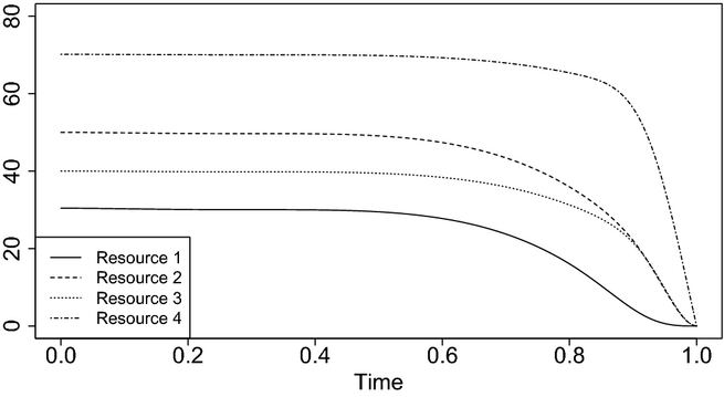
ASOCP Bid Prices Trajectories for a 4 Resource Network

Numerical Experiments

In this section, we present the results from three sets of numerical experiments. The experiments compared the performance of various bid price control policies used to make accept/reject decisions for a simulated stream of customers. The purpose of these experiments were to provide empirical answers to the following questions:

How do discrete time dynamic bid prices compare to continuous time dynamic bid prices in a continuous time setting?

How do continuous time dynamic bid prices perform in comparison to LP bid prices that are re‐optimized a sufficient number of times?

Are continuous time dynamic bid prices scalable to industrial sized networks?

The first two questions were analyzed using network structures similar to the problem instances in Adelman (2007). Each spoke had flights traveling to and from the hub, departing at the end of the booking horizon. For cases with more than one hub, each hub had flights traveling to and from the other hub(s). These flights made up the network's resources. If H was the number of hubs in the network and L was the number of spokes, then the total number of resources in the network was the sum of the number of hub‐spoke legs and the number of hub‐hub legs. Thus, the network had m = 2HL + H(H − 1) single‐leg flights. The set of products for each network included all possible OD itineraries. Both high‐fare and low‐fare tickets were offered for each OD pair. The load factor was calculated as the expected demand for seats over all itinerary divided by the capacity of the network and was equal to

\int_{0}^{T} \sum_{j} λ_{j, t} A_{j} d t / c m

. The main difference between our experiments and Adelman's was that time was continuous and scaled to the interval [0, 1].

The third set of experiments utilized the Porter Airlines' schedule to create an industrial scale network. Porter Airlines is a regional airline based in Toronto, Canada, with hubs in Toronto, Montreal, Ottawa, and Halifax. The airline provides “short haul” flights to cities in Ontario, Quebec, and Atlantic Canada, as well as cities in the United States, including daily flights to Boston, Newark, and Chicago. Since Porter's business model emphasizes service, speed, and convenience for business and leisure travelers, the airline offers frequent flights between major Canadian and US cities, flying up to 20 times daily from Toronto to Ottawa and 11 times daily from Toronto to Newark‐New York. The experiments over the Porter Airlines network demonstrate the potential of the ASOCP as a solution method for problems of industrial size.

All solution methods for each set of experiments were executed through SHARCNET, a high‐performance Canadian research computing consortium. The first set of experiments was run on the SHARCNET serial throughput cluster Kraken using single threaded AMD Opteron 2.2 GHz processors. The second and third sets of experiments, which have larger networks and re‐optimization, were run on the SHARCNET serial throughput cluster ORCA using 8 threaded Intel Xeon 2.7 GHz processors. For further details on the experimental design and additional documentation of the results please see Appendix S3.

Fixed Bid Price Experiments

The first set of experiments examines whether discrete time dynamic bid prices provide a suitable control policy when customer arrivals occur in continuous time. To analyze this question, fixed bid price control policies from the LP, DLP, and ASOCP were used to generate revenues from a simulated stream of customers modeled by a Poisson process. We chose to use the dynamic disaggregation (DD) approach to solve the DLP, since the approach represents state of the art computational efficiency for dynamic bid prices. The numerical experiments in Vossen and Zhang (2015) demonstrated that the DD is the fastest method for producing dynamic bid prices in discrete time. The DD approach produces time‐dependent bid prices by solving the LP and adding variables and constraints simultaneously to the problem until optimality is obtained. Since the DLP bid prices are constant for the majority of the booking horizon, the dynamics of the bid prices are captured entirely by the columns and rows added in the constraint generation procedure. For brevity, we refer the reader to section 3 of Vossen and Zhang (2015) for a complete description of the DD algorithm and optimization problems. To approximate the Poisson process in discrete time, we set the probability of an arrival, ρ, to 0.8 producing a discrete booking horizon of

\frac{λ}{ρ}

periods. For reference, Adelman (2007) fixed the probability of an arrival at 0.8 in his experiments and Vossen and Zhang (2015) fixed the probability of an arrival to 0.9 in their experiments. For computing the ASOCP we set

K = {0, 0.8, 0.9, 1}

N_{k} = 50

, and Ω = 0.05.

The bid price policies were tested on a 1 hub 3 spoke (six resources and 24 products) network. Similar to Cooper (2002) and Jasin and Kumar (2013) the problems were scaled by the parameter κ, such that the capacity was

c = κ c_{0}

and the expected arrivals were

λ = κ λ_{0}

. The expected arrivals and capacity had base values of

λ_{0} = 40

customers and

c_{0} = 6

seats per flight, which corresponded to a load factor of 1.678. The problems were varied by scale factors κ ∈ {1, 2, 5, 10, 20}. The demand for each OD pair was stationary. The probability that an itinerary request was for a low‐fare (high‐fare) class ticket was 0.75 (0.25). The prices for low‐fare products were randomly drawn from the set [20, 50] with equal probability. The high‐fare products were priced at five times the corresponding low fare. Each pair of network parameters was simulated 1000 times. The experiments only considered fixed bid price controls, implying that each method was solved at t = 0 and the resulting bid prices were used to make product acceptance decisions for the entire booking horizon.

Table 1 reports the upper bound on the revenue, the simulated revenues for each bid price policy, and the average run‐times for fixed bid price experiments. The objective value of the DD was selected as the upper bound, since DD provides a tighter upper bound compared to the LP. For each network, the ASOCP generated the highest revenue, capturing between 87.6–93.5% of the upper bound, while the LP and DD captured 79.2–84.8% and 83.8–86.7% of the upper bound, respectively. Although the ASOCP generates greater revenue relative to the DD when arrivals are in continuous time, the run‐time of the DD is considerably faster. The ASOCP's average run‐time across the various scale factors ranged within 20–60 times the run‐time of the DD. From the standpoint of a fixed bid price policy, the DD offers a compromise relative to the LP and ASOCP in terms of the revenue vs. run‐time performance tradeoff. There is a distinct revenue improvement relative to the LP, with a substantial run‐time improvement relative to the ASOCP.

Table 1

Revenue and Run‐Time in Seconds for Fixed Bid Price Experiments

	Upper bound	Average revenue			Average run‐time
κ		LP	DD	ASOCP	LP	DD	ASOCP
1	4524	3587	3791	3963	0.0005	0.0195	0.4145
2	9227	7551	7812	8289	0.0003	0.0093	0.4421
3	23,323	19,503	20,075	21,488	0.0005	0.0085	0.4992
4	46,812	39,495	40,360	43,512	0.0003	0.0130	0.5311
5	93,790	79,501	81,320	87,731	0.0008	0.0143	0.5645

To account for the stochastic nature of demand and capacity consumption, airlines update capacity vectors and re‐optimize bid prices periodically throughout the booking horizon. Consequently, when airlines solve for the optimal bid prices, the capacity of each resources is unlikely to be balanced. For either the DD or ASOCP to be a functional solution method for dynamic bid prices, the run‐times should not change significantly when the available capacities across resources vary. To test the DD and ASOCP performance given asymmetric capacities, the first set of experiments was re‐simulated with randomized capacities such that

\sum_{i \in I} c_{i} = 6 κ c_{0} and c_{i} \in [κ (c_{0} - ν), \dots, κ (c_{0} + ν)], \forall i \in I . (45)

(45)

The parameter ν controls variability in the capacity vectors. For ν ∈ {1, 2, 3, 4}, each set of demands, prices, and arrival paths was simulated for 10 randomized capacity vectors satisfying condition 45.

Table 2 reports the average run‐times for the DD and ASOCP across the different values of ν and κ. For each value of κ, the average DD run‐time appears to increase substantially. The run‐times for ν = 4 increase with κ and range between 45 − 187 times the run‐times for ν = 1. On the other hand, the ASOCP run‐times for ν = 4 are 1.003 − 1.782 times the run‐times for ν = 1. These distinct behaviors result from the structure of dynamic bid prices and substantial differences in computing methodology. Theorem 2 of Adelman (2007) states that the value of the bid price for a given resource is static from the start of the booking horizon until a critical time where the bid price becomes dynamic. As the capacity vectors increase in variability, select flight legs become scarcer at the start of the horizon. Bookings for these resources have a greater impact on the dynamics of the bid price, resulting in the critical times occurring earlier in the booking horizon as ν increases. Therefore, as the capacity vectors increase in variability, the DD requires adding a greater number of rows and columns before the algorithm terminates. On the other hand, the ASOCP considers the entire booking horizon using the spline approximation regardless of the capacity vector. Thus, there is little impact on the algorithm's timing and it is fairly robust to variation in capacity. Finally, despite the dramatic increase in run‐time for the DD, Table 3 shows that the average revenue is still less than the revenue generated by the ASOCP. Since the run‐times increase as the variability in the starting capacity grows, we conclude that the DD is at a disadvantage for situations with frequent updating and unbalanced capacities, when arrivals occur in continuous times.

Table 2

Run‐Time in Seconds for Fixed Bid Price Experiments with Asymmetric Capacities

	ν = 1		ν = 2		ν = 3		ν = 4
κ	DD	ASOCP	DD	ASOCP	DD	ASOCP	DD	ASOCP
1	0.0208	0.4986	0.0333	0.5024	0.2054	0.5986	0.9509	0.8887
2	0.0405	0.5353	0.0657	0.5321	0.3028	0.5493	2.5630	0.5983
3	0.0621	0.6010	0.0784	0.5941	1.4724	0.6045	9.7771	0.6031
4	0.0838	0.6792	0.1276	0.6410	2.1020	0.6543	17.8454	0.6814
5	0.1178	0.6541	0.1557	0.7169	1.8977	0.6995	33.8710	0.6697

Table 3

Revenue for Fixed Bid Price Experiments with Asymmetric Capacities

	ν = 1		ν = 2		ν = 3		ν = 4
κ	DD	ASOCP	DD	ASOCP	DD	ASOCP	DD	ASOCP
1	3786	3926	3767	3869	3674	3761	3501	3563
2	7726	8230	7728	8154	7541	7878	7420	7703
3	20,189	21,579	20,212	21,359	19,609	20,489	19,424	20,348
4	40,351	43,370	40,509	42,732	39,977	42,064	38,790	41,015
5	81,760	87,685	82,187	86,438	81,028	84,841	77,502	81,978

Bid Price Experiments with Updates

In a study comparing the behavior of LP heuristics, Jasin and Kumar (2013) provide theoretical results that advocate using LP bid prices over the asymptotically optimal booking limit heuristics, provided that the LP is resolved sufficiently frequently. For the ASOCP to have value as a bid price solution method, it must be able to provide higher revenues than the LP bid price control that is updated sufficiently often throughout the booking horizon. To ensure adequate updating, we re‐optimized the LP at uniformly spaced intervals as many times as the expected number of arrivals over the course of the booking horizon. On the other hand, we limited the number of optimization updates for the ASOCP to 10 (also at evenly spaced intervals) in order to keep the run‐time for both bid price controls at a similar order of magnitude. The experiments establish that the ASOCP provides an effective bid price policy and demonstrates the value of time‐dependent bid price compared to static bid prices that are updated repeatedly.

The experiment networks consisted of H ∈ {1, 2, 3} hubs connected to L = 3 spokes. The initial capacity for each single‐leg flight was c = 150. The arrival rates λ were varied in order to produce different load factors. For the one hub experiments λ ∈ {1000, 1100, 1200}, for the two hub experiments λ ∈ {1600, 1800, 2000}, and for the three hub experiments λ ∈ {2400, 2600, 2800}. Each network was simulated 500 times with the bid price policies facing identical customer arrivals modeled by a Poisson process with the same parameters as described in subsection 6.1.

Similar to the fixed bid price experiments in subsection 6.1, we evaluated the performance of the ASOCP by benchmarking revenues against the LP. The average revenues and the upper bound as well as the run‐times and remaining inventory are listed in Table 4. The percentage of the revenue generated by the LP relative to the LP bound ranged from 96.5% to 98.5%, with an average of 97.6%, while the revenue percentage for the ASOCP ranged from 98.4% to 99.4%, with an average of 99.1%. The low performance gap is due to the asymptotic optimality of the LP Bound; however, the ASOCP is still able to provide a revenue boost compared to LP bid prices. Under a direct comparison of bid price policy performance, the ASOCP provided an average improvement from 0.81% to 2.58% (1.01% across the entire set). Although the total run‐time was 25 times larger on average, with the LP being updated 1000–2800 times, the solution time for each network was under a minute, which is reasonable considering the revenue improvements. The experiments also show that ASOCP can achieve good performance with limited updating, unlike the LP, which requires frequent re‐optimization. Another interesting observation is that the LP had a higher utilization of resources for each network. This implies that a significant amount of the ASOCP revenue improvement stems from denying product requests in favor of reserving capacity for more profitable itineraries.

Table 4

Revenue and Run‐Time in Seconds for Multi‐Hub Network with Updates

Network {h,m,n}	Load factor	Upper bound	Average revenue		Total run‐time
			LP	ASOCP	LP	ASOCP
{1,6,24}	1.636	57534	55728	56879	0.132	2.144
	1.796	62136	59988	61485	0.149	1.988
	1.969	66250	64225	65880	0.162	2.081
{2,14,112}	1.558	94207	92391	93305	0.378	6.199
	1.789	98634	97072	97997	0.42	6.525
	1.975	107561	105,042	105,947	0.457	6.891
{3,24,264}	1.478	142088	139,936	141,066	0.962	54.394
	1.602	150922	147,440	148,839	1.032	54.976
	1.737	157033	154,100	155,662	1.4979	52.687

Porter Airlines Network

We simulated bid prices using the ASOCP and LP over an entire day in Porter's network, which consisted of 182 single‐leg flights and 1098 possible itineraries. Table 5 provides a list of Porter's single‐leg flights and their frequency of service on December 1, 2011. We consider the network with one fare class and two fare classes for each itinerary. Similar to subsections 6.1 and 6.2, the booking horizon was scaled to the interval [0, 1] and time was continuous. The capacity of each flight was 70 seats, coinciding with Porter's fleet of Bombardier Q400 aircraft and the expected demand over the entire network for both the single and two‐fare cases was given by λ = 12000. The LP and ASOCP optimization problems were optimized ϕ ∈ Φ≡{5, 10, 20, 35} times at uniform intervals over the booking horizon. The Porter network was simulated 200 times, with randomly sampled expected demand and price for each itinerary (see the Appendix for details).

Table 5

List of Single‐Leg Flights for Porter Airlines Network (December 1, 2011)

Departure city	Arrival city	Number of flights
Boston (BOS)	Toronto (YTZ)	7
Chicago (MDW)	Toronto (YTZ)	6
Halifax (YHZ)	Montreal (YUL)	2
Halifax (YHZ)	Ottawa (YOW)	5
Halifax (YHZ)	St John's (YYT)	4
Moncton (YQM)	Toronto (YTZ)	1
Montreal (YUL)	Halifax (YHZ)	2
Montreal (YUL)	Toronto (YTZ)	18
Newark (EWR)	Toronto (YTZ)	11
Ottawa (YOW)	Halifax (YHZ)	5
Ottawa (YOW)	Moncton (YQM)	1
Ottawa (YOW)	Toronto (YTZ)	20
Quebec City (YQB)	Toronto (YTZ)	3
Sault Ste Marie (YAM)	Toronto (YTZ)	3
St John's (YYT)	Halifax (YHZ)	4
Sudbury (YSB)	Toronto (YTZ)	3
Thunder Bay (YQT)	Toronto (YTZ)	5
Toronto (YTZ)	Boston (BOS)	7
Toronto (YTZ)	Chicago (MDW)	6
Toronto (YTZ)	Montreal (YUL)	18
Toronto (YTZ)	Newark (EWR)	11
Toronto (YTZ)	Ottawa (YOW)	20
Toronto (YTZ)	Quebec City (YQB)	3
Toronto (YTZ)	Sault Ste Marie (YAM)	3
Toronto (YTZ)	Sudbury (YSB)	3
Toronto (YTZ)	Thunder Bay (YQT)	5
Toronto (YTZ)	Windsor (YSG)	3
Windsor (YSG)	Toronto (YTZ)	3

Table 6 compares the revenues and run‐time for the LP and ASOCP bid price controls. For both one fare and two fare class problems, the ASOCP produced higher revenues than the LP bid price for each ϕ ∈ Φ. In addition, for a single fare class, the ASOCP‐based policy with ϕ = 5 generated more revenue than each LP‐based policy. The improvement offered by the ASOCP ranged between 0.27–3.37% and 0.26–0.53% for the one and two‐fare class problems, respectively. Although the ASOCP run‐times are several orders of magnitude greater than the LP run‐times, we argue that the ASOCP is a promising approach for solving large‐scale capacity control problems. Airlines have access to superior computational power through industrial server farms and work stations, which would increase the optimization speed for computing ASOCP bid prices. On the other hand, airlines are restricted in the number of times that they can re‐optimize bid prices. Bid price controls involve extensive scenario analysis and constant monitoring, often leaving bid prices to be computed overnight (Talluri and van Ryzin 2004). If the booking horizon represents a 10‐week period and optimization occur overnight, then the values of ϕ ∈ {5, 10, 20, 35} corresponds to re‐optimizing the bid prices once every two weeks, once a week, twice a week, and every other day, respectively, over the 10‐week period. From this perspective, on the nights when the airline updated the bid prices, the average run‐time, regardless of the number of fare classes was under 25 seconds. Finally, SOCP solvers have not evolved to the same extent as LP solvers in terms of solution speed. As SOCP solvers mature, the ASOCP will become even more viable as a solution method for computing bid prices for industrial networks.

Table 6

Average Revenue and Run‐Time in Seconds per Optimization for the Porter Airlines Experiments

	1 Fare revenue		2 Fare revenue		1 Fare run‐time		2 Fare run‐time
ϕ	LP	ASOCP	LP	ASOCP	LP	ASOCP	LP	ASOCP
5	1,044,910	1,080,080	2,901,300	2,916,650	0.0048	11.852	0.0048	14.356
10	1,065,150	1,080,120	2,919,470	2,927,040	0.0042	18.638	0.0049	20.449
20	1,074,400	1,080,130	2,928,510	2,939,570	0.0044	16.216	0.0047	19.225
35	1,077,800	1,080,750	2,931,960	2,942,420	0.0045	17.821	0.0048	23.383

Conclusion and Future Research

In this article, we construct a bid price control policy starting from a continuous time network RM framework. After substituting the optimal control policy into the HJB equation and reformulating it as a differential inclusion, we introduce two approximations into the inclusion to establish the AOCP. Using the monotonicity of the bid prices, approximation theory is used to develop the ASOCP, which makes the number of variables independent of the time horizon. Finally, we employ an efficient constraint generation procedure allowing the ASOCP to produce time‐dependent bid prices by considering only a select number of time‐capacity vectors. The numerical experiments highlight the effectiveness of the proposed approach in generating bid prices as well as its scalability by solving problems on an industrial sized network. Future research could extend the ASOCP structure to incorporate customer choice. It would also be interesting to combine ASOCP with robust optimization to incorporate uncertainty in the arrival rates. The ASOCP not only has the potential to improve revenues for large airlines, but its methodology can be applied to other areas of RM and large‐scale approximate optimal control problems.

Footnotes

Acknowledgments

This research was supported in part by the Natural Sciences and Engineering Research Council of Canada (grant number 341412‐2011) and Queen's School of Business. The authors thank the Department and Senior Editors, and the Referees for their constructive suggestions, which helped to improve the results. The computational component was made possible by the facilities of the Shared Hierarchical Academic Research Computing Network (SHARCNET:http://www.sharcnet.ca) and Compute/Calcul Canada.

References

Adelman

. 2007. Dynamic bid‐prices in revenue management. Oper. Res. 55(4): 647–661.

Akan

., Ata

. 2009. Bid‐price controls for network revenue management: Martingale characterization of optimal bid prices. Math. Oper. Res. 34(4): 912–936.

Alizadeh

., Eckstein

Noyan

Rudolf

. 2008. Arrival rate approximation by nonnegative cubic splines. Oper. Res. 56(1): 140–156.

Alizadeh

., Goldfarb

. 2003. Second‐order cone programming. Math. Programm. 95(1): 3–51.

Bitran

., Caldentey

. 2003. An overview of pricing models for revenue management. Manuf. Serv. Oper. Manag. 5(3): 203–229.

Bremaud

. 1981. Point Processes and Queues. Springer‐Verlag, New York.

Cooper

. 2002. Asymptotic behavior of an allocation policy for revenue management. Oper. Res. 50: 720–727.

Jasin

., Kumar

. 2013. Analysis of deterministic LP‐based booking limit and bid price controls for revenue management. Oper. Res. 61(6): 1312–1320.

Karlin

., Studden

. 1966. Tchebycheff Systems, with Applications in Analysis and Statistics. Wiley, New York.

10.

Kunnumkal

., Topaloglu

. 2008. A refined deterministic linear program for the network revenue management problem with customer choice behavior. Nav. Res. Logisti. 55(6): 563–580.

11.

Kunnumkal

., Topaloglu

. 2010. Computing time‐dependent bid prices in network revenue management problems. Transport. Sci. 44(1): 38–62.

12.

Lieb

., Loss

. 2001. Analysis. American Mathematical Society.

13.

Liu

., Van Ryzin

. 2008. On the choice‐based linear programming model for network revenue management. Manuf. Serv. Oper. Manag. 10(2): 288–310.

14.

Loewen

., Rockafellar

. 1994. Optimal control of unbounded differential inclusions. SIAM J. Control Optim. 32(2): 442–470.

15.

López

., Still

. 2007. Semi‐infinite programming. Eur. J. Oper. Res. 180(2): 491–518.

16.

Meissner

., Strauss

. 2012. Network revenue management with inventory‐sensitive bid prices and customer choice. Eur. J. Oper. Res. 216(2): 459–468.

17.

Rhys

J. M. W

. 1970. A selection problem of shared fixed costs and network flows. Manage. Sci. 17(3): 200–207.

18.

Still

. 2001. Discretization in semi‐infinite programming: the rate of convergence. Math. Programm. 91(1): 53–69.

19.

Talluri

., van Ryzin

. 2004. The Theory and Practice of Revenue Management. Kluwer Academic Publishers, Norwell, MA.

20.

Tong

., Topaloglu

. 2014. On approximate linear programming approach for network revenue management problems. INFORMS J. Comput. 26: 121–134.

21.

Topaloglu

. 2009. Using Lagrangian relaxation to compute capacity‐dependent bid‐prices in network revenue management. Oper. Res. 57(3): 637–649.

22.

Vinter

. 2000. Optimal control . Systems & Control: Foundations & Applications, Birkhäuser, Boston, MA.

23.

Vossen

., Zhang

. 2015. A dynamic disaggregation approach to approximate linear programs for network revenue management. Prod. Oper. Manag. 24(3): 469–487.

24.

Wolkowicz

., Saigal

Vandenberghe

, eds. 2000. Handbook of Semidefinite Programming: Theory, Algorithms and Applications. Kluwer, Dordrecht, The Netherlands.

25.

Zhang

., Adelman

. 2009. An approximate dynamic programming approach to network revenue management with customer choice. Transport. Sci. 42(3): 381–394.