Increasing Supply Chain Robustness through Process Flexibility and Inventory

Abstract

We study a hybrid strategy that uses both process flexibility and finished goods inventory for supply chain risk mitigation. The interplay between process flexibility and inventory is modeled as a two‐stage robust optimization problem. In the first stage, the firm allocates inventory before disruption happens; in the second stage, after a disruption happens, the firm determines production quantities at each plant to minimize demand loss. Our robust optimization model can be solved efficiently using constraint generation, and under some stylized assumptions, can be solved in closed form. For a canonical family of flexibility designs known as the K‐chains, we provide an analytical expression for the optimal inventory solution, which allows us to study the effectiveness of different degrees of flexibilities. Moreover, we find that firms should allocate more inventory to high variability products when its level of flexibility is low, but as flexibility increases, the inventory allocation pattern “flips” and firms should allocate more inventory to low variability products. These observations are further verified through a numerical case study of an automobile supply chain. Finally, we extend our robust optimization model to the time‐to‐survive metric, a metric that computes the longest time a supply chain can guarantee a predetermined service level under disruption.

Keywords

supply chain risk process flexibility inventory robust optimization

Introduction

Over the past decade, managing supply chain disruption risks has emerged as one of the top business challenges. As reported by Forbes, 80% of companies worldwide see better protection of supply chains as a priority (Culp 2013). Supply chain disruption is difficult to manage because it can come from a wide range of sources, whether from natural disaster, epidemics, factory fire or political upheavals (Simchi‐Levi et al. 2014). The problem is further exacerbated as new sources of disruptions are constantly emerging, exemplified by the recent Equifax data breach (O’Marah 2017) and the computer system outage at Delta Air Lines (Jansen 2017).

To effectively manage supply chain risks, a firm needs to coordinate different risk mitigation strategies under supply and demand uncertainty. In this study, we focus on two popular risk mitigation strategies: holding finished goods inventory and employing process flexibility. While it is clear that both strategies improve supply chain resilience, it is much more challenging to understand the hybrid approach that combines both strategies. Therefore, for a firm to successfully implement the hybrid approach, one needs to answer the following questions: how does the firm's flexibility design affect its inventory decisions? And how should the firm allocate inventory among different products to achieve a required service level while minimizing cost?

To study the hybrid strategy, we introduce a two‐stage robust optimization model in which finished goods inventory is stored in the first stage, while in the second stage, after disruption happens, the firm decides what and how much to produce at each plant using process flexibility to minimize the impact of disruption. Our two‐stage risk mitigation model is intended for relatively infrequent disruption events, in contrast to stochastic dynamic models that are used to model frequent disruptions, e.g., (Tomlin 2006). In our model, the second‐stage decisions represent the firm's actions during a disruption, and the first‐stage inventory decisions represent the inventory levels the firm wants to build up prior to disruptions. Moreover, the inventory flexibility strategy we consider is most practical when a firm is facing disruptions that last for a short term, e.g., a few weeks, as holding months of inventory is a very expensive risk mitigation strategy. For longer term disruptions, the firms may consider our inventory flexibility strategy as an intermediate solution, while remodeling their supply chains to resume production quickly. For example, after the 2011 Japanese Earthquake, Toyota started to create a quake‐proof supply chain that is guaranteed to recover in less than two weeks when another disruption occurs (Kim 2011).

Risk Mitigation Strategies

Next, we provide basic intuitions behind the two risk mitigation strategies, process flexibility and inventory, and then explain why it is important to coordinate the two strategies.

Risk mitigation inventory, also known as protective inventory, has been identified in a number of papers as an important tool for dealing with supply chain risk (see literature review in section 1.4). However, holding a large amount of inventory would incur a high loss in cost efficiency (Chopra and Sodhi 2014), as these inventories are only used when disruptions occur. As a result, firms would typically hold the minimum amount of inventory subject to a given performance requirement.

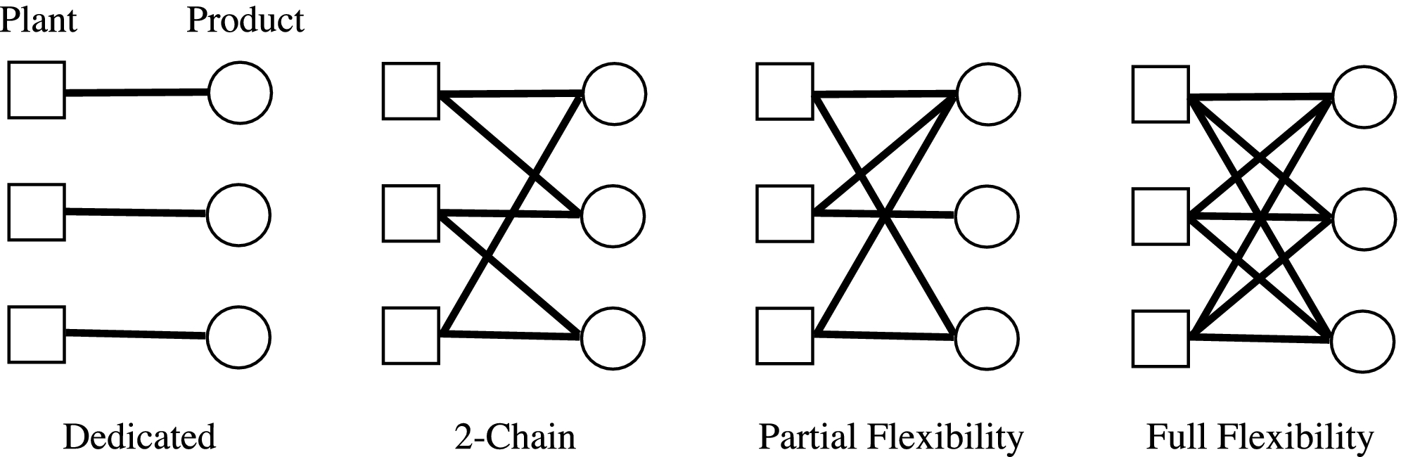
Process flexibility is defined as the “ability to build different types of products in the same manufacturing plant or on the same production line at the same time” (Jordan and Graves 1995). For example, under full flexibility design, each plant is capable of producing all products; while under dedicated design (i.e., no process flexibility), each plant is capable of producing just a single product (see Figure 1).

Figure 1

Process Flexibility Designs

With process flexibility, the firm is capable of adjusting its production in the existence of uncertainties, and thus, is in a better position to match its capacity and demand. Unfortunately, implementing full flexibility is often too expensive since each plant needs to be capable of producing all products (Simchi‐Levi 2010). As a result, partial flexibility designs are considered. A popular class of partial flexibility designs studied in the literature are known as K‐chains (Hopp et al. 2004, Chou et al. 2014). In a K‐chain, there are N plants and N products, and for each 1 ≤ i ≤ N, plant i has the flexibility to produce products i, i + 1, to i + K − 1 modulo N (see Figure 1 for an example of 2‐chain). Note that if K = 1, we get dedicated design in the N plants and N products system, and if K is equal to the number of products, we get full flexibility design.

It is important to note that process flexibility can greatly impact inventory decisions. Consider dedicated and full flexibility designs in Figure 1 as an example. Suppose that the firm holds inventory for Product 2, and a disruption occurs at Plant 1. Then, under dedicated design, the inventory of Product 2 would not be helpful, since the inventory cannot be used to satisfy any of the demand for Product 1. However, under full flexibility design, inventory of Product 2 can be used to save the flexible production capacities at Plant 2, which allows the firm to reallocate the capacities at Plant 2 to produce Product 1. In other words, when a firm has both inventory and process flexibility, inventory helps to free up excess flexible capacities during an unforeseen event, and thus improves the firm's ability to mitigate risk. As a result, the existence of process flexibility can reduce the amount of inventory needed, and the synergy between inventory and process flexibility makes the hybrid strategy very compelling.

Although it is well documented that both flexibility and inventory can improve supply chain resilience (see literature review in section 1.4), the synergy between inventory and process flexibility is not well understood. To the best of our knowledge, no existing literature has considered a hybrid strategy combining (partial) process flexibility designs and inventory as a way to mitigate against risks in a multi‐product supply chain. We note that because holding extra amounts of inventories can be inefficient and expensive, our hybrid strategy is mainly intended for infrequent disruptions when the firm can restore its original production capacity in a few weeks. In the latter part of the article, we will also discuss how process flexibility may greatly increase the effectiveness of inventories, and potentially allow firms to use this strategy for longer disruptions.

Robust Optimization Model

In both process flexibility and risk mitigation literature, uncertainties in demands and capacities are typically specified through probability distributions. Given probability distributions, the firm's objective is modeled using two different approaches. In the first approach, the firm's objective is to maintain a high level of profit/production with high probability (aka Type 1 service level). In this case, the inventory and process flexibility problem would be modeled as a two‐stage stochastic program with chance constraints. Unfortunately, these service constraints are non‐convex (see Appendices S1–S2 for more details), which makes the stochastic problem intractable. A different approach is to minimize the firm's expected cost. This would lead to a two‐stage linear stochastic program, which is a convex optimization problem. However, even for discrete distributions, solving the two‐stage linear stochastic program exactly is #P‐hard (Dyer and Stougie 2006), and practitioners would often resort to approximating the true problem, using sample average approximation (SAA). The quality of the SAA solutions depends on the number of samples, and the number of samples required for SAA solutions to achieve strong theoretical guarantees is often very large (Shapiro and Nemirovski 2005). Therefore, SAA is only capable of producing good solutions for problems with a small number of variables.

In the interest of computational tractability, we propose a two‐stage robust optimization model that finds the optimal inventory allocation under general process flexibility designs. In the robust optimization model, product demands and plant capacities lie in an uncertainty set. In the first stage, given a process flexibility design, the firm allocates its inventory levels across the products; and in the second stage, after the uncertainties are realized, the firm uses both inventory and process flexibility to either minimize its cost or satisfy a certain service level requirement. We find this robust model to be more tractable than its stochastic counterparts. In our numerical example (section 4), we find that two‐stage robust problems for supply chains can be solved much faster than its stochastic counterparts. In some stylized settings, our robust model can even be solved in closed form (section 3), allowing for detailed analysis in order to identify useful insights. Finally, further computational experiments demonstrate that our robust model containing hundreds of nodes can be solved to optimality in less than 10 minutes (see chapter 4 of Wang 2016).

Apart from tractability, the worst‐case model provides several additional advantages compared with its stochastic counterparts in the context of risk mitigation. First, it is difficult and often impossible to accurately assess the uncertainties in plant disruptions, because production disruption can occur from so many different sources, whether from natural disaster, epidemics, or factory fire (Simchi‐Levi et al. 2014). Because the optimal inventory level can be very sensitive to the probability of disruption, considering the worst‐case scenario may offer a more “robust” approach. Second, for small probability events such as plant disruptions, managers might find it useful to understand the maximum possible shortage of demand under a wide range of scenarios. This understanding may lead them to better identify scenarios where the supply chain is most vulnerable. Finally, it has been suggested in Graves and Willems (2000) that it is easier for managers to communicate with customers by committing to a certain service level under a range of scenarios, rather than providing a probabilistic guarantee, which is difficult to understand or verify.

Overview and Summary of Results

Robust Optimization Model. In section 2, we propose a robust optimization formulation for supply chain risk mitigation. The decision variables are inventory levels in the first stage and production quantities in the second stage. The formulation ensures that the total demand lost is bounded by some target value for all scenarios in the uncertainty set, with the objective of minimizing the inventory costs. It turns out that our formulation is highly tractable numerically, and under some stylized assumptions, can be even solved in closed form. We also demonstrate that our model can be extended in several ways in section 5. In particular, our model can be extended to find the optimal inventory allocation that maximizes a supply chain's time‐to‐survive (TTS), a metric that measures the longest time the supply chain can maintain customer service levels.

Analysis and Insights. In section 3, we analyze a special family of flexibility designs called the K‐chains to provide insights into inventory allocations under different degrees of flexibility. First, we provide a closed‐form characterization of the optimal inventory decision when the uncertainty set is symmetric. Using this characterization, we find that while changing from a dedicated network to the well‐studied 2‐chain design provides a large portion of benefit, when plants are subject to disruptions, two‐chain does not completely capture the benefit of full flexibility even under moderate demand variabilities, and there are significant benefits achieved by increasing the degree of flexibility beyond two‐chain. The characterization also allows us to understand how the gap between inventory costs of 2‐chain and K‐chain (K > 2) changes when we vary the magnitude of potential disruptions.

Second, we show that the optimal inventory allocation can be drastically different under different flexibility designs. In particular, there tends to be a shift of inventories from high variability products to low variability products as the degree of process flexibility increases. We refer to such phenomenon as the flipping effect, since the inventory levels flip as the degree of flexibility increases. Therefore, it is unlikely that a single inventory strategy can perform well for all kinds of flexibility designs. Optimizing over inventory decisions that are tailored to the firm's particular supply chain network structure using our robust optimization model may significantly improve the firm's risk mitigation strategy, compared with other simple inventory heuristics that ignore the firm's supply chain structure.

Numerical Case Study. In section 4, we apply our robust optimization approach to a risk mitigation example of General Motors. The example is based on a real‐world case introduced by Jordan and Graves (1995). The numerical experiment supports our finding that 2‐chain is not as effective as K‐chain for K > 2 when there is supply uncertainty, even when the assumptions in section 3 do not hold. We also demonstrate the flipping effect in this numerical case study.

Related Literature

There is rich literature on inventory for risk mitigation. Many of the earlier papers (e.g., Meyer et al. 1979, Song and Zipkin 1996, Arreola‐Risa and DeCroix 1998) studied inventory risk mitigation in a single product setting. More recently, inventory mitigation strategies under multi‐period, multi‐echelon settings have also been explored (e.g., Bollapragada et al. 2004, DeCroix 2013). Moreover, researchers have also considered hybrid strategies in which firms use both dual sourcing and inventory to mitigate risks (Gürler and Parlar 1997, Tomlin 2006).

Process flexibility, also referred to as “mix flexibility” or “product flexibility”, has also been observed as a potential risk mitigation tool. Tomlin and Wang (2005) consider a risk mitigation strategy that uses a combination of mix‐flexibility and dual sourcing. Tang and Tomlin (2008) suggest process flexibility as one of the five types of flexibility strategies that can be used to mitigate supply chain disruptions. And finally, Sodhi and Tang (2012) list flexible manufacturing processes as one of the eleven robust supply chain strategies.

While many researchers investigated the effectiveness of fully flexible resources (e.g., Fine and Freund 1990, Bish and Wang 2004, Tomlin and Wang 2005), our model allows one to study arbitrary partial process flexibility designs in a multi‐plant, multi‐product system. This feature is motivated by the seminal work of Jordan and Graves (1995), who argue that fully flexible resources are often too expensive or impossible to implement, while a little bit of flexibility in the system often provides the same benefit as full flexibility. More recently, the effectiveness of sparse flexibilities designs have been verified by a number of theoretical developments (e.g., Chou et al. 2010,2011, Simchi‐Levi and Wei 2012, Wang and Zhang 2015). Moreover, Bassamboo et al. (2010,2012) observed that when the firm is free to purchase any flexible resource, sparse configurations such as chaining and tailored pairing are often near optimal.

Production postponement and delayed product differentiation is another stream of literature closely related to the two‐stage flexibility and inventory model we study. The classical research of Fisher and Raman (1996) and Swaminathan and Tayur (1998) studied two‐stage production models, but neither paper proposed a model that incorporates partial second‐stage production flexibility. To the best of our knowledge, the only paper in the postponement literature that considers partial flexibility is the work of Chou et al. (2014). However, that work differs from our article significantly as they focused on a stochastic model with no capacity uncertainties, whereas our paper studies a robust model with capacity disruptions.

In this article, we propose a robust optimization approach to study the risk mitigation strategy for combining partial process flexibility and inventory. The model is a two‐stage robust optimization problem, where the firm allocates inventory before the uncertainties are realized (ex ante), and schedules its flexible production after uncertainties are realized (ex post). Our approach to model uncertainties follows the recent proposals in the robust optimization literature (e.g., Ben‐Tal et al. 2009, Bandi and Bertsimas 2012), which propose to replace probabilistic distributions with uncertainty sets. This approach is similar to the model studied by Graves and Willems (2000), who argued that in supply chain management, it is often easier for the firm to commit to service level guarantees under a range of scenarios, rather than probabilistic service guarantees.

In the two‐stage robust optimization literature, Ben‐Tal et al. (2004) studied general two‐stage robust linear programs (which they called “Adjustable Robust Counterpart”). They proved that the two‐stage robust linear programs are NP‐hard in general, and proposed the Affine Adjustable Robust Counterpart, which is shown to be computationally tractable in many settings. Atamtürk and Zhang (2007) studied a general two‐stage robust network flow problem, showing that while the problem is NP‐hard in general, it can yield polynomial‐timed solutions when the networks have certain structures. Computational methods for solving general two‐stage robust linear programs include, for example, Thiele et al. (2010), who proposed a cutting‐plane method, and Zeng and Zhao (2013), who proposed a column‐and‐constraint generation algorithm. For a more detailed overview of the recent advances and applications of two‐stage robust optimization, we refer readers to the surveys by Bertsimas et al. (2011) and Gabrel et al. (2014).

The Model

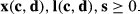
We consider a firm that has M plants (denoted by

S_{i}

for i = 1, …, M) and produces N products (denoted by

T_{j}

for j = 1, …, N). A plant may produce either one or multiple products, and the flexibility design specifies which product each plant can produce. More formally, the firm's flexibility design can be represented as a bipartite network, where a link

(S_{i}, T_{j})

exists if and only if plant i is able to produce product j. We refer to the set of such links as

F

. For a given flexibility design

F

and a subset of products

A \subset {T_{1}, \dots, T_{N}}

, we define

P_{F} (A) = {S_{i} : (S_{i}, T_{j}) \in F, T_{j} \in A}

as the plants that can produce at least one of the products in A.

We assume that both plant capacity and product demand are uncertain quantities due to unknown risks such as plant disruptions or demand fluctuations. We denote the realized capacity by c = (c ₁, c ₂, …, c _M), and the realized demand by d = (d ₁, d ₂, …, d _N). We use

U \subset R_{+}^{M} \times R_{+}^{N}

to denote the uncertainty set for both capacity and demand, and assume

(c, d) \in U

. Throughout the article, we will consider polyhedral uncertainty sets; that is,

U

will be defined by a set of linear inequalities.

Service Guarantee Model

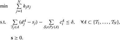
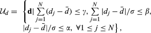
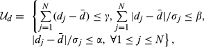
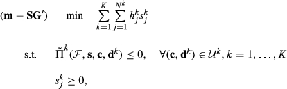
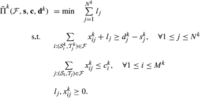
Next, we present the service guarantee (SG) model, where the firm ensures that total demand loss for any scenario in uncertainty set

U

is bounded by a fixed shortage allowance, δ, while minimizing inventory cost. This can be modeled using a two‐stage decision problem. In the first stage, the firm determines inventory level for each product, where the inventory level of product j is denoted by variable s _j, with unit holding cost h _j. In the second stage, the firm observes realized product demand and available plant capacities, and determines its production schedule. We use x _ij(c, d) to denote the quantity of product j produced by plant i under demand d and capacity c. Similarly, we use l _j(c, d) to denote the lost sales of product j. The inventory decision problem can then be formulated as follows.

\begin{matrix} (SG) min_{s, x, l} & \sum_{j = 1}^{N} h_{j} s_{j} \\ s.t. & \sum_{i : (S_{i}, T_{j}) \in F} x_{ij} (c, d) + l_{j} (c, d) \geq d_{j} - s_{j}, \\ \forall 1 \leq j \leq N, (c, d) \in U, \\ \sum_{j : (S_{i}, T_{j}) \in F} x_{ij} (c, d) \leq c_{i}, \\ \forall 1 \leq i \leq M, (c, d) \in U, \\ \sum_{j = 1}^{N} l_{j} (c, d) \leq δ, \forall (c, d) \in U, \end{matrix}

(1)

x (c, d), l (c, d), s \geq 0 .

(2)

The first constraint defines lost sales where demand is satisfied by either production or inventory, and the second constraint enforces plant capacity limits. The third constraint ensures that the total lost sales is bounded by a fixed budget δ.

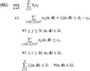
While the SG model defines service guarantee aggregated over all products, the model can also be used if the firm requires service guarantees on an individual product level. To do this, we need to make two changes in the model: first, the lost sales allowance δ is set to zero; second, the uncertainty set

U

is modified to reflect service guarantee for individual products. For example, if the firm wants to commit to 95% of the demand for each product under all possible scenarios in uncertainty set

U

, then we can define the uncertainty set to

U^{'}

, where

U^{'} = {(c, 0.95 d) | (c, d) \in U}

. Note that the uncertainty set

U^{'}

can easily be modified to allow different products having different service guarantee levels (by making an affine transformation on

U

Optimization Algorithm

We claim that the service guarantee model (SG) can be solved efficiently using an optimization method called constraint generation. Because this article is focused on deriving operational insights on the interplay between flexibility and inventory, we omit the technical details of the algorithm to solve the robust optimization model; instead, we only give an outline of the algorithm. Full details of the constraint generation algorithm can be found in chapter 4 of Wang (2016).

The algorithm for solving the SG model can be divided into two main steps. First, we can reformulate the two‐stage robust optimization problem associated with the SG model as the following linear program:

\begin{matrix} min & \sum_{j = 1}^{N} h_{j} s_{j} \\ s.t. & \sum_{T_{j} \in A} (d_{j}^{A} - s_{j}) - \sum_{S_{i} \in P_{F} (A)} c_{i}^{A} \leq δ, \forall A \subset {T_{1}, \dots, T_{N}}, \\ s \geq 0 . \end{matrix}

(3)

The derivation of this reformulation can be found in chapter 4 of Wang (2016). Note that this linear program has N variables and 2^N linear constraints (with one constraint associated with each subset of the N products;

d_{j}^{A}

and

c_{i}^{A}

are constants defined for each subset A), so the number of constraints grows exponentially as the number of products increases. When N is not a large number, we can directly solve the linear programming formulation 3. However, in general when N > 15, solving 3 with all the 2^N constraints becomes extremely slow.

To solve the SG model faster, in the second step, we apply a constraint generation algorithm to the linear programming problem 3. We provide the basic ideas of our algorithm here. The constraint generation algorithm for solving the SG model runs iteratively, starting from a linear program with the same objective function as in 3 but with an empty set of constraints. At each iteration, the algorithm first solves the linear program with objective 3 and the current set of constraints, then runs a subroutine that either proves that the current inventory vector s is optimal, or returns a violating linear constraint in 3. Depending on the outcome of the subroutine, the algorithm either terminates with an optimal solution, or adds another inequality to the current set of constraints. When the uncertainty set is polyhedral, the subroutine can be reformulated as a compact mixed integer linear program (MILP) (see chapter 4 of Wang (2016) for details), which can be solved quickly, using off‐the‐shelf optimization solvers. In general, the algorithm stops when only a tiny fraction of the 2^N constraints are added to the set, so the running time of the constraint generation algorithm (and the running time of the subroutines) is much shorter than the time to solve the full linear programming formulation with exponentially many constraints. For example, when the number of products is equal to 50 and the uncertainty set is polyhedral, the full linear programming formulation has 2⁵⁰ ≈ 1.12 × 10¹⁵ constraints, and solving a linear program with this size is beyond the capability of any existing LP solvers. In contrast, we observe in numerical experiment that our constraint generation algorithm requires only (on average) a few hundred constraints being generated, even if the LP contains more than 10¹⁵ constraints; furthermore, each constraint generation step takes a fraction of a second. For a detailed discussion of the computational complexity of the algorithm, we refer readers to chapter 4 of Wang (2016).

We note that while constraint generation is a common standard technique for solving linear programs with a large number of constraints (Bertsimas and Tsitsiklis 1997), different tricks are often needed to come up with the subroutine that efficiently generates constraints depending on specific problem structures. In our constraint generation algorithm, we take advantage of the network flow structure to come up with a subroutine that solves a mixed‐linear integer program with moderate size. Finally, while we focus on the SG model in the article, our computational algorithm can be applied to more general models with different lost sales costs for different products, or multiple stages of productions. These extensions are discussed in section 5.

Constructing Uncertainty Sets for Stochastic Fluctuations

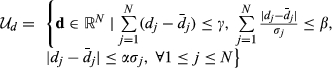
So far, we have introduced a robust optimization formulation of the supply risk mitigation problem, and our model framework allows using any polyhedral uncertainty set (i.e., a finite set of linear inequalities) to model demand and supply uncertainty. Typically, in robust optimization, the uncertainty set is chosen based on some probabilistic interpretation (Bertsimas and Thiele 2006). In this section, we introduce a specific class of parametric uncertainty sets and discuss how to choose the values of the uncertainty set parameters in applications. For the rest of the article, we will mainly focus on this class of uncertainty sets.

We start with the demand uncertainty. In the literature, product demands are often described as stochastic quantities. Suppose that the demand for each product j is denoted by some random variable D _j with mean

{\bar{d}}_{j}

and standard deviation σ _j. In this case, applying the method described by Ben‐Tal et al. (2009), we use the following set of linear inequalities to restrict the variations of demand, d.

\begin{matrix} \sum_{j = 1}^{N} (d_{j} - {\bar{d}}_{j}) \leq γ, \sum_{j = 1}^{N} \frac{| d_{j} - {\bar{d}}_{j} |}{σ_{j}} \leq β, | d_{j} - {\bar{d}}_{j} | \leq α σ_{j}, \\ \forall 1 \leq j \leq N . \end{matrix}

(4)

The constraint defined by parameter γ allows us to upper‐bound the maximum total demand increase compared with the mean. The constraint defined by parameter β is known as the budgeted uncertainty constraint, and allows us to control the total normalized deviation between the actual demand and its mean. Finally, the constraints defined by parameter α is known as box uncertainty constraints and allow us to control demand deviations for each individual product. The values of α, β and γ can be chosen based on empirical data or probability theories such as the central limit theorem (Ben‐Tal et al. 2009). Alternatively, the parameters can be chosen in order to optimize or estimate stochastic quantities (Bertsimas and Thiele 2006, Bandi and Bertsimas 2012). To avoid negative product demand, we assume throughout the article that

α σ_{j} \leq {\bar{d}}_{j}

for any 1 ≤ j ≤ N.

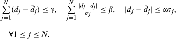
The uncertainty set equation 4 includes several types of commonly used uncertainty sets as special cases. For instance, one may consider a box uncertainty set where each demand variable d _j is bounded individually, which is a special case of equation 4 with β = γ = +∞. The budget uncertainty set is also a special case of equation 4 with β = +∞.

Although we will focus on demand uncertainty sets defined by equation 4 in the rest of the article, we note that other forms for demand uncertainty set can be used in our model. A possibility is bounding the standard deviation of demands instead of the absolute deviation of demands as in equation 4. However, this modification involves quadratic constraints in the uncertainty set. When the uncertainty set contains only linear inequalities as in equation 4, the optimization algorithm (described in section 2.2) can be implemented efficiently by solving a sequence of mixed integer linear programs (MILPs). If the uncertainty set is a quadratic conic set, our algorithm requires solving a sequence of mixed integer conic quadratic programs (MICQPs). Although there are several open‐source solvers for MICQPs, the dimensions of solvable MICQP by current solvers are much smaller compared to MILPs (Bonami et al. 2012).

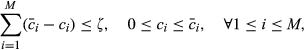
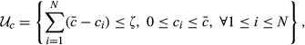
In the context of risk mitigation, most of the capacity uncertainty comes from plant disruptions due to low probability, unforeseeable events. Because standard deviations of the disruptions are difficult to estimate and plant disruptions may cause the entire plant to go down, we do not consider the budgeted uncertainty constraint to the capacity vector. Moreover, because plant capacities can only decrease due to disruption, we use the following set of inequalities to restrict the capacity vector, c,

\sum_{i = 1}^{M} ({\bar{c}}_{i} - c_{i}) \leq ζ, 0 \leq c_{i} \leq {\bar{c}}_{i}, \forall 1 \leq i \leq M,

(5)

where parameter ζ bounds the total loss of capacity for all of the plants. Alternatively, we can view ζ as the firm's judgment on the potential magnitude of a disruption.

In the rest of this article, we will focus on the uncertainty set

U

defined by Equations 4 and 5. For more techniques to construct uncertainty sets, we refer interested readers to Bandi and Bertsimas (2012) and the references therein.

Analysis and Insights

In the previous section, we proposed a robust optimization framework that coordinates inventory and production decisions to mitigate supply disruptions. To further understand this robust optimization approach, we study two stylized settings based on the service guarantee (SG) model. In both settings, we assume that the number of plants and products are equal (M = N), all products have a unit holding cost (h _j = 1), and the demand shortage parameter is zero (δ = 0). Note that δ bounds the aggregate demand loss. As we commented in section 2.1, even when δ = 0, demand loss for individual products can still be included in the model by making an affine transformation to the uncertainty set.

Inventory Costs under Different Flexibility Levels

To analyze different flexibility levels, we consider the K‐chain designs. The K‐chains are commonly studied in the literature (e.g., Hopp et al. 2004, Chou et al. 2014, Wang and Zhang 2015) as a class of designs with different levels of flexibility. Recall that in a K‐chain, for each 1 ≤ i ≤ N, plant i has the flexibility to produce products i, i + 1, to i + K − 1 modulo N. If K = 1, we get dedicated design in the N by N system, and if K is equal to the number of products, we get full flexibility design.

We use the class of uncertainty sets defined by Equations 4 and 5 in section 2.3, and assume that the uncertainty is symmetric, that is,

\bar{d_{j}} = \bar{d}

, σ _j = σ and

c_{i} = \bar{c}

, for all 1 ≤ j ≤ N. Under our assumption, any

U

can be expressed as

U = U_{c} \times U_{d}

, where

\begin{matrix} U_{d} = & \{d | \sum_{j = 1}^{N} (d_{j} - \bar{d}) \leq γ, \sum_{j = 1}^{N} | d_{j} - \bar{d} | / σ \leq β, \\ | d_{j} - \bar{d} | / σ \leq α, \forall 1 \leq j \leq N\}, \end{matrix}

(6)

U_{c} = \{c | \sum_{i = 1}^{N} (\bar{c} - c_{i}) \leq ζ, 0 \leq c_{i} \leq \bar{c}, \forall 1 \leq i \leq N\},

(7)

for some parameters γ, ζ, β and α.

Under these assumptions, we can obtain a closed‐form analytical expression for the optimal inventory of the SG model for K‐chains. Let e be a vector with all entries equal to 1. For any integer 1 ≤ t ≤ N, we define

\begin{matrix} C^{min} (t) & = min_{x} {c^{T} x ∣ e^{T} x \geq t, 0 \leq x \leq 1, c \in U_{c}}, \\ (N = 8, \bar{d} = \bar{c} = 1, α = 2, β = γ = 4) \\ D^{max} (t) & = max_{x} {d^{T} x ∣ e^{T} x \leq t, 0 \leq x \leq 1, d \in U_{d}} . \end{matrix}

Proposition 1

Let

F

be a K‐chain, for some integer 1 ≤ K ≤ N. Then the optimal inventory cost of the SG model is

\begin{matrix} N max \{max_{1 \leq t \leq N - K} \frac{D^{max} (t) - C^{min} (t + K - 1)}{t}, \\ max_{N - K < t \leq N} \frac{D^{max} (t) - C^{min} (N)}{t}, 0\} . \end{matrix}

(8)

The characterization for the optimal inventory cost of K‐chain in Proposition 1 provides us with a useful tool to think about the effectiveness of different degrees of flexibility. For example, it allows us to solve the optimal inventory cost of K‐chains by solving N linear programs, which is much faster than the constraint generation algorithm for the general SG model. In addition, the characterization allows us to further analyze the optimal cost for a K‐chain as we change different parameters. In Figure 2, we plot an example of the inventory cost as magnitude of a disruption (measured by ζ) changes, under different levels of demand variability σ and different flexibility designs including 2‐chain, 3‐chain and full flexibility. The reason why we consider the impact of ζ is because its value is typically difficult to estimate, as disruption may come from many different sources. From another perspective, one can view ζ as a firm's conservativeness thinking about disruption ‐ larger ζ would imply that the firm is planning more conservatively as it prepares for disruptions impacting a larger portion of its production capacity.

Figure 2

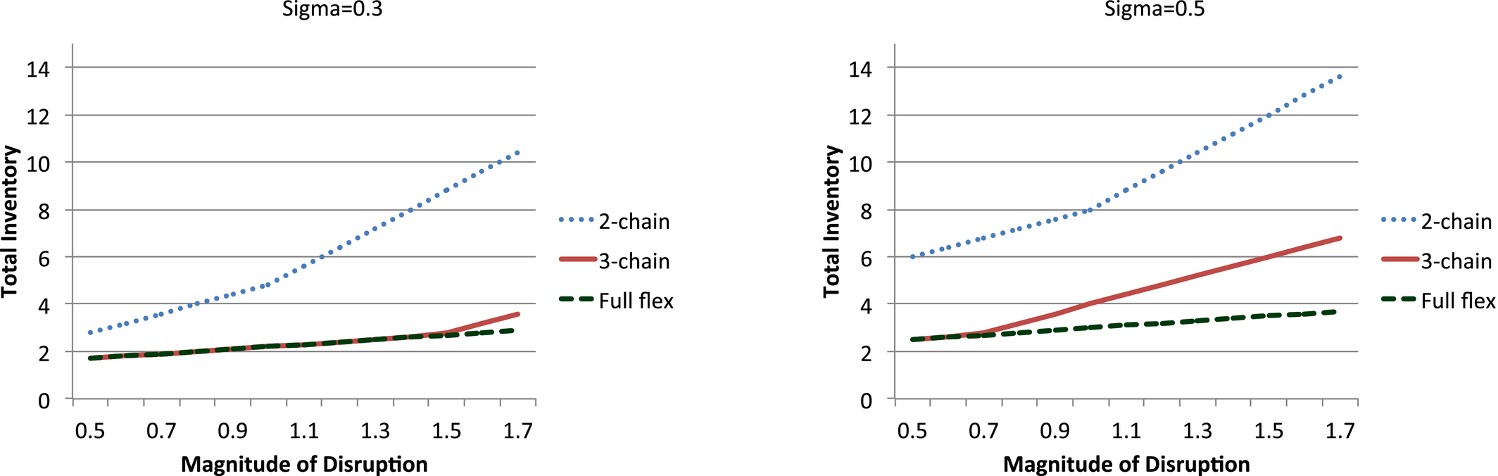
Inventory Cost for K‐chain Designs [Color figure can be viewed at wileyonlinelibrary.com]

From Figure 2, we observe that there is a significant gap between the performance of 2‐chain and K‐chain for K > 2 with both capacity and demand uncertainty. This contrasts to the classical observations that 2‐chain performs almost as well as full flexibility (and hence K‐chain for any K > 2) when there is no capacity uncertainty (Jordan and Graves 1995). For illustration, in the 10 plants 10 products example studied by Jordan and Graves (1995), if demand is normally distributed with coefficient of variation of 0.4, then the expected utilization rate of full flexibility is 95.4%, while that of 2‐chain is already 95%. In comparison, the optimal inventory of 2‐chain in Figure 2 is more than twice that of full flexibility, under most of the parameter ranges.

Interestingly, we also observe that most of the gap between 2‐chain and full flexibility can be closed by 3‐chain, which is just one additional degree of flexibility higher than 2‐chain. In hindsight, this is not entirely surprising. Intuitively, while 2‐chain is very effective in satisfying uncertain demand without capacity uncertainty, even the disruption of a single production plant can break up the chain; in comparison, 3‐chain would still form a chain even if one plant is down. We note that recent findings suggest that 2‐chain may not be effective when the demand variability is large compared with capacity (Chou et al. 2014,Wang and Zhang 2015). A crucial difference between our observation to the existing literature is that in our setting, a relatively small amount of uncertain supply disruption, e.g., shutdown of a single plant, creates a significant gap between 2‐chain and full flexibility, as illustrated in Figure 2 under moderate demand variability (σ = 0.3).

Given that there is a significant gap between 2‐chain and K‐chain for K > 2 with both capacity and demand uncertainty, another interesting question is the comparative static of this gap and potential capacity loss. From Figure 2, we observe that when capacity loss (measured by ζ) increases, the gap between the inventory costs for 2‐chain and K‐chain (K > 2) widens. Next, we formally prove this observation under a wide range of ζ.

Proposition 2

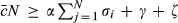
When

0 \leq ζ \leq 2 \bar{c}

, the difference between the optimal inventory costs of 2‐chain and K‐chain (K > 2) is increasing as ζ increases.

Proposition 2 is useful for a decision maker (DM) thinking about adding flexibility in the following way: suppose that the DM is considering between 2‐chain and 3‐chain but is unsure about the potential capacity loss caused by disruptions, which is described by ζ. Then, the DM can always calculate the difference between the inventory costs of 2‐chain and 3‐chain under the minimum (maximum) reasonable ζ, and this quantity would indeed be a lower‐bound (upper‐bound) on the difference under other values of ζ, as long as

0 \leq ζ \leq 2 \bar{c}

. Finally, in the following corollary, we show that if

ζ > 2 \bar{c}

, then the optimal inventory costs of 2‐chain is the same as dedicated design. Thus, when

ζ > 2 \bar{c}

, the firm should ignore 2‐chain completely, and consider either implementing flexibility with more than 2 degrees, or not implementing flexibility at all.

Corollary 1

When

ζ > 2 \bar{c}

, the optimal inventory costs of 2‐chain is equal to ND ^max(1), which is equal to the optimal inventory costs of a dedicated design.

The intuition behind Corolary 1 is reasonably straightforward. Consider product 1. Intuitively, in the worst‐case scenario for product 1, both plants capable of producing product 1 are disrupted, while product 1 has demand D ^max(1). This forces us to allocate D ^max(1) amount of inventory at product 1. By symmetry of 2‐chain, we also need to allocate D ^max(1) amount of inventory at product 2, 3, …, N, which is exactly the optimal inventory allocation for the dedicated design.

Inventory Allocation Strategy

In this section, we study a setting where product demand variability is different. Like section 3.1, we consider a special case of the uncertainty set defined in section 2.3 given by

\begin{matrix} U_{d} = & \{\sum_{j = 1}^{N} (d_{j} - \bar{d}) \leq γ, \sum_{j = 1}^{N} | d_{j} - \bar{d} | / σ_{j} \leq β, \\ | d_{j} - \bar{d} | / σ_{j} \leq α, \forall 1 \leq j \leq N\}, \end{matrix}

(9)

U_{c} = \{\sum_{i = 1}^{N} (\bar{c} - c_{i}) \leq ζ, 0 \leq c_{i} \leq \bar{c}, \forall 1 \leq i \leq N\},

(10)

with

U = U_{c} \times U_{d}

. The parameter σ _j measures the demand variability of product j.

We want to understand how inventory allocations change as we add more flexibility to the system, starting from a dedicated flexibility design. First, for dedicated design (K = 1), we show that under the optimal decision, the firm places more inventories to the high variability products.

Proposition 3

When

F

is a dedicated design (i.e., 1‐chain), there always exists an optimal inventory solution s, such that for any two products

j_{1}, j_{2}

with

σ_{j_{1}} \geq σ_{j_{2}}

, we have

s_{j_{1}} \geq s_{j_{2}}

In contrast, for full flexibility design (K = N), it can be shown that the optimal inventory allocation places more inventories to the low variability products, under a large range of parameters.

Proposition 4

When

F

is a full flexibility design (i.e., N‐chain), if

\bar{c} N \geq α \sum_{j = 1}^{N} σ_{i} + γ + ζ

, there always exists an optimal inventory solution s, such that for any two products

j_{1}, j_{2}

with

σ_{j_{1}} \geq σ_{j_{2}}

, we have

s_{j_{1}} \leq s_{j_{2}}

We note that condition

\bar{c} N \geq α \sum_{j = 1}^{N} σ_{i} + γ + ζ

is usually satisfied in practice: ζ (the loss of capacity due to disruption),

α \sum_{j = 1}^{N} σ_{i}

(total absolute demand deviation), and γ (total demand variation) all measure the variability of the system; due to the central limit theorem, all three quantities are usually smaller than

\bar{c} N

, the total capacity of the system, because the total capacity scales linearly in N and variability scales in the order of

\sqrt{N}

. Moreover, a condition of this form is necessary—for example, if

\bar{c} N < ζ

, then the uncertainty set would contain scenarios where the total available capacity is zero, rendering any flexibility design useless.

Propositions 3 and 4 demonstrate that if we start from dedicated design and add flexibilities until we arrive at full flexibility, the inventory allocations to high and low variability products will be eventually flipped. We call this the flipping effect, which is the phenomenon that the optimal solution holds more inventory for products with high demand variability when the degree of flexibility is low, but holds more inventory for products with lower variability when the firm has a high degree of flexibility, and thus the pattern of inventory decision “flips” as the degree of flexibility grows. The intuition behind the flipping effect is that when there is full flexibility, the firm is more concerned about being able to use inventory to free up capacities anywhere in the system because any capacity is fully flexible, therefore placing more inventories to low variability products so that the inventories can be consumed when needed. On the contrary, when there is dedicated design, the firm should place inventories to high variability products, in order to ensure its service level.

We also note that Propositions 3 and 4 do not require the assumption that the capacity loss is positive (ζ > 0), suggesting that demand variability is the main driver for the flipping effect. In section 4, we further confirm this insight as our numerical studies show that the flipping effect also holds when we have deterministic capacity loss, as well as when demand variation and capacity loss are stochastic.

The flipping effect has also been partially observed in production postponement under stochastic demand, as Fisher and Raman (1996) showed that when the second stage production is fully flexible, the firm should produce more low variability products in the first stage. However, Fisher and Raman (1996) do not consider the change in inventory allocations as flexibilities are added into dedicated design. Our finding augments Fisher and Raman (1996), and demonstrates that when the firm adds flexibility to its manufacturing system, its optimal inventory allocation strategy can change drastically, with the trend of allocating more inventories to low variability products. The flipping effect also demonstrates that when a manufacturing system has partial process flexibility, there does not exist a universal rule‐of‐thumb method for inventory allocation. In these cases, our model and computational algorithm provide a tool for effectively making optimal inventory decisions.

The placement of inventories to low variability products in full flexibility is also related to the push and pull strategy in the operations management literature (see, e.g., Simchi‐Levi 2010). In a pull strategy, the firm produces to order after demand is realized. In a push strategy, the firm produces to stock and has less ability to adjust. With full flexibility, the firm should apply pull strategy to products with high demand uncertainty, and apply push strategy to products with low demand uncertainty, which means holding more inventory for products with lower variability in the first stage.

Application: Risk Mitigation for an Automotive Supply Chain

In this section, we apply our robust optimization method to a case study for automobile supply chains. We consider an automotive manufacturing system based on the General Motors data provided by Jordan and Graves (1995). The dataset consists of 16 vehicle models and 8 assembly plants. We use the same plant capacities and mean product demands as in their paper, shown in the left hand side of Figure 3. Since the dataset does not include cost information, we apply the service guarantee (SG) model, and assume all products have a unit holding cost.

Figure 3

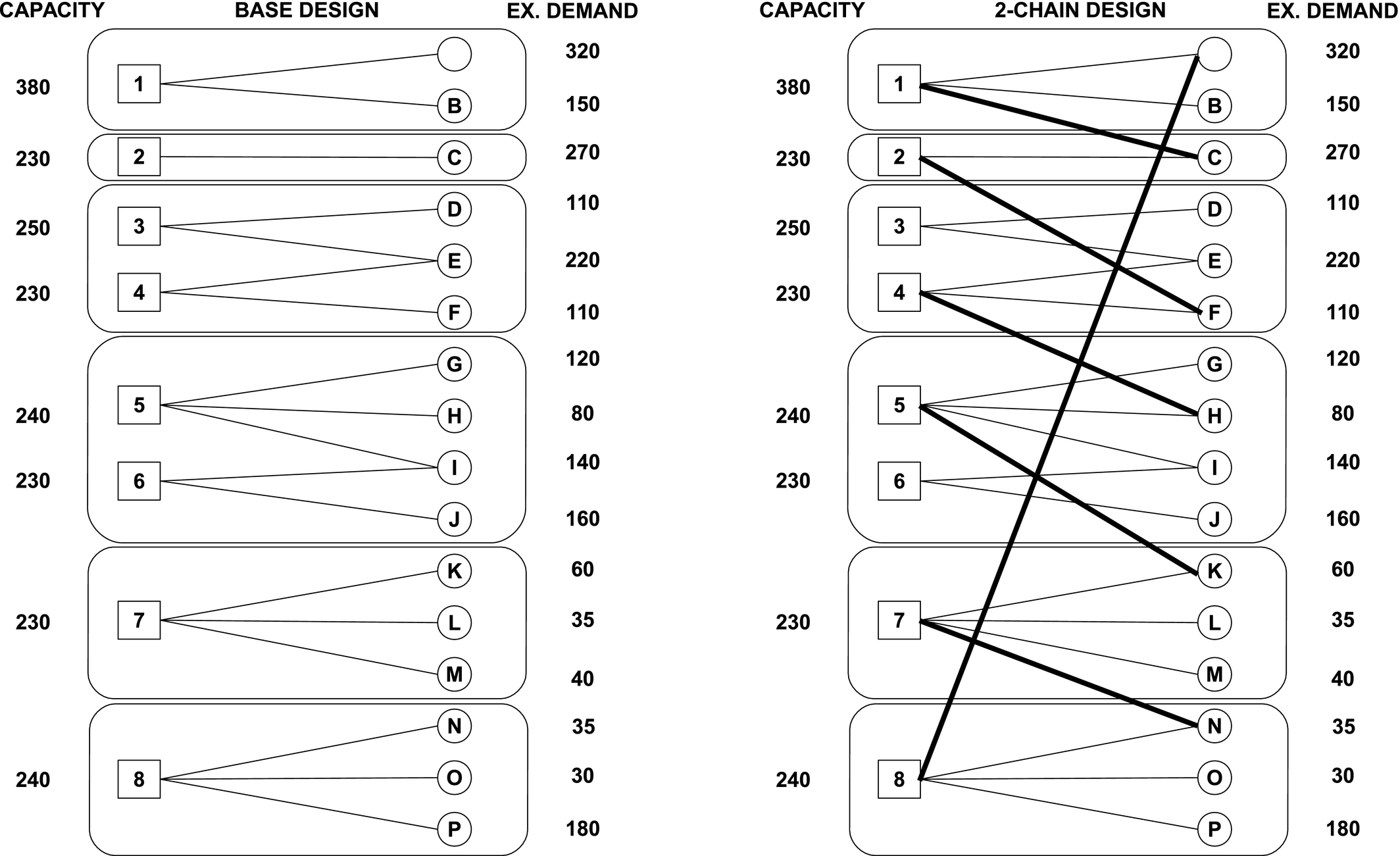
Flexibility Design in the GM Example

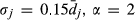
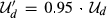
The uncertainty set is created according to the section 2.3, with parameters α, β, γ, and ζ. We present our findings with parameters set to α = 2, β = 8 and

γ = 0.5 \sum_{j = 1}^{N} σ_{j}

. Furthermore, we assume at most 10% of total capacity may be lost under plant disruption, namely,

ζ = 0.1 \sum_{i = 1}^{M} {\bar{c}}_{i}

. The demand shortage allowance δ is set to 5% of the total mean demand. While we only present our numerical results under this set of parameter values, we have also tested a wide range of different parameter values within 50% of the presented values. For all of the different sets of values tested, we obtained similar qualitative insights.

To simulate the scenarios where products have different demand variability, we assume that half of the products have high variability demand with

σ_{j} = v_{h} {\bar{d}}_{j}

, and the rest of products have low variability demand with

σ_{j} = v_{l} {\bar{d}}_{j}

, where v _h > v _l > 0. We tested three groups of variabilities: (v _h, v _l) = (0.2, 0.1), (0.3, 0.15), and (0.4, 0.2). In each case, we test 200 scenarios where high variability products are randomly selected.

To study systems with different flexibility levels, we construct flexibility designs based on the K‐chain design in balanced (M = N) systems. Recall that in a K‐chain design, plant i is capable of producing products i, i + 1, to i + K − 1. Since the number of plants and products are unequal in this example, we construct “generalized K‐chains” by following the clustering idea of Jordan and Graves (1995). More specifically, Jordan and Graves (1995) proposed clustering plants and products into separate groups (six groups in this example), and consider each group as a plant dedicated to producing one product family. Once clustered, the base design can then be viewed as a dedicated or 1‐chain design. Finally, to create a generalized K‐chain, for each group i, one adds flexibility arcs to connect group i to groups i + 1, …, i + K − 1. An example of the generalized 2‐chain is given in the right side of Figure 3.

There are many ways to add flexibility links to create a generalized K‐chain design: the resulting design depends on the order that the groups appear in the chain, as well as plants and products being connected in each group. Because not all flexible designs are feasible due to physical and technological limitations, and these limitations may differ across different firms, in our simulation, we do not use the optimal K‐chain. Instead, for each of the 200 scenarios, we generate a generalized K‐chain by randomly selecting a group permutation, and then connect a random plant in each group i to a random product in each of the groups i + 1, …, i + K − 1. Finally, we also consider full flexibility design, where any plant can produce all products. Note that full flexibility design contains M × N = 128 flexibility arcs, while the base design, 2‐chain, 3‐chain, and 4‐chain contains 16, 24, 32, and 40 flexibility arcs, respectively.

Tables 1 and 3 list the optimal total inventory cost and the percentage of inventory allocated to high variability products (averaged over 200 random instances) respectively. We start with the observation from Table 1. From Table 1, we see that while changing from the base design to a 2‐chain design reduces inventory cost, there is also significant inventory cost reduction from a 2‐chain design to designs with higher degrees of flexibility, such as 3‐chain or 4‐chain. This observation echoes the insight from our analysis in section 3.1, which shows that in the presence of supply disruption, 2‐chain is no longer as effective as full flexibility.

Table 1

Total Inventory Cost

(v _h, v _l)	Base	2‐chain	3‐chain	4‐chain	Full
(0.2, 0.1)	1219.5 (439%)	573.1 (206%)	343.8 (124%)	292.9 (105%)	277.9
(0.3, 0.15)	1514.3 (430%)	786.4 (224%)	497.4 (141%)	405.2 (115%)	351.8
(0.4, 0.2)	1809.0 (425%)	1014.1 (238%)	670.7 (158%)	535.1 (126%)	425.7

Note: The percentages in round brackets display the cost ratios of the designs to full flexibility.

We also want to illustrate that the uncertainty in supply significantly increases the ineffectiveness of a 2‐chain, compared with systems that suffer from deterministic loss in capacity. To illustrate this, we test another numerical example with the same setting, except that all plant capacities are deterministic and set to 90% of their original capacity levels. The result is shown in Table 2. Note that full flexibility design has the same inventory cost in Tables 1 and 2, because the two examples assume the same worst‐case total capacity. However, the performance of 2‐chain is much better in Table 2. Therefore, we conclude that as capacity uncertainty increases, 2‐chain becomes less effective.

Table 2

Total Inventory Cost (Deterministic Capacity)

(v _h, v _l)	Base	2‐chain	3‐chain	4‐chain	Full
(0.2, 0.1)	526.2 (189%)	331.6 (119%)	277.9 (100%)	277.9 (100%)	277.9
(0.3, 0.15)	784.3 (223%)	510.4 (145%)	360.6 (103%)	355.1 (101%)	351.8
(0.4, 0.2)	1047.5 (246%)	706.6 (166%)	474.9 (112%)	445.3 (105%)	425.7

Note: The percentages in round brackets display the cost ratios of the designs to full flexibility.

Next, we discuss the percentages of inventories allocated to high variability products (Table 3). Recall that in every example, 8 products are randomly selected with high demand variability

σ_{j} = v_{h} {\bar{d}}_{j}

, and the remaining 8 products have low variability demand

σ_{j} = v_{l} {\bar{d}}_{j}

. For different variability parameters (v _h, v _l), the result shows the same trend: the optimal solutions hold more inventory for products with high demand variability when the degree of flexibility is low (e.g., base design). But as the degree of flexibility increases (e.g., 4‐chain, full flexibility), it is optimal to hold more inventory for products with lower variability, and to hold less inventory for products with higher variability. The simulation result verifies the flipping effect observed in section 3.2, furthermore, the percentages of inventories allocated to high variability products are monotonically decreasing as we add flexibility to the system. In general, the flipping effect occurs gradually as we add flexibility to the system, and the magnitude of the flipping depends on the variabilities of the products. Interestingly, we find that the flipping effect is not unique to systems with capacity uncertainty. In Table 4, we list the percentages of inventories allocated to high variability products when capacities are deterministically reduced by 10%. As Table 4 shows, the flipping effect still exists when there is no capacity uncertainty.

Table 3

Percentage of Inventory for High Variability Products

(v _h, v _l)	Base	2‐chain	3‐chain	4‐chain	Full
(0.2, 0.1)	50.1%	49.8%	48.4%	45.6%	41.3%
(0.3, 0.15)	51.4%	52.0%	50.1%	46.2%	38.8%
(0.4, 0.2)	53.9%	54.7%	52.0%	47.6%	33.0%

Table 4

Percentage of Inventory for High Variability Products (Deterministic Capacity)

(v _h, v _l)	Base	2‐chain	3‐chain	4‐chain	Full
(0.2, 0.1)	50.8%	43.6%	42.2%	41.5%	41.3%
(0.3, 0.15)	53.9%	47.2%	41.6%	39.8%	38.8%
(0.4, 0.2)	57.3%	51.0%	43.2%	37.2%	33.0%

Furthermore, we note that the findings above are not unique to the robust optimization model, as similar results also hold for the stochastic model (see Appendix S2 for a description of the model). In the stochastic model, we consider a case where product demands are independent and normally distributed truncated at two standard deviations. We assume that 8 randomly selected products have high variability demands with a coefficient of variation equal to 0.5; the remaining 8 products have a coefficient of variation equal to 0.25. We assume that each plant is disrupted independently with probability 0.1. The objective is to find the optimal inventory allocation such that the expected fill rate is at least 95%. The model is solved by the SAA method (described Appendix S2) with 1000 samples.

Compared with the robust optimization model, the stochastic model takes much longer to solve. For this example with 16 vehicle models, the robust optimization model is solved by constraint generation in less than a second, while the SAA approach takes about 10 minutes. For a large scale network with hundreds of nodes, the robust optimization model can still be solved in a few minutes on a standard laptop, while the SAA model becomes prohibitively large to solve.

Table 5 shows the total inventory level and the percent of the inventory allocated to high variability products, averaged over 200 random examples. The result provides similar qualitative insights obtained from the robust optimization model: (1) there is a significant improvement in inventory cost when more flexibility is added to the 2‐chain; (2) less and less inventory is allocated to high demand variability products as the degree of flexibility increases.

Table 5

Inventory Allocation for the Stochastic Model

	Base	2‐chain	3‐chain	4‐chain	Full
Total inventory	902.4	485.3	335.8	299.6	269.0
High var products	44.4%	42.5%	40.2%	34.9%	13.1%

Extensions to the Service Guarantee Model

Time‐to‐Survive Model

In this subsection, we introduce a metric called Time‐to‐Survive (TTS) to measure the resilience of supply chain when the duration of the disruption is unknown. Given a facility in the supply chain (e.g., a plant or a distribution center), TTS is defined as the longest time that customer service level is guaranteed if this facility is disrupted. The TTS metric has already been adopted by the Ford Motor Company to assess risk exposure in its complex supply chain and evaluate Ford's risk mitigation strategies (Simchi‐Levi et al. 2014,2015).

The definition of TTS is motivated by the concept of Time‐to‐Recover (TTR), which is the time for a facility to return to full capacity after a disruption. TTR is widely used to evaluate supply chain risk (see e.g., Hopp et al. 2012). If TTS is greater than TTR, then a disruption in that facility is not going to affect the firm's service level. On the other hand, when TTS for a specific facility is shorter than TTR, then a disruption at that facility will have an impact on service. Thus, an important challenge in supply chain risk management is to allocate inventory to different products to increase the supply chain's time to survive.

For this purpose, we define the supply chain TTS as the minimum (worst) TTS among all of the potential scenarios. The longer the supply chain TTS, the more robust the supply chain is.

Below we show that the problem of allocating inventory to maximize supply chain TTS can be reduced to a special case of the model in section 2.

Suppose that plant i has capacity c _i per unit time (i = 1, …, M), product j has a demand rate d _j per unit time (j = 1, …, N). Let r _j be the amount of inventory allocated to product j, and assume that the sum of inventory among all products cannot exceed a given budget R. We use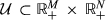

U \subset R_{+}^{M} \times R_{+}^{N}

to denote the uncertainty set that models the uncertainty of plant capacity and product demand. We then formulate the problem of maximizing supply chain TTS as the following nonlinear program:

\begin{matrix} (TTS) & max_{r_{j}, x_{ij}^{(c, d)}} t \\ s.t. & t \leq \frac{r_{j}}{d_{j} - \sum_{i : (i, j) \in F} x_{ij}^{(c, d)}}, \\ \forall 1 \leq j \leq N, (c, d) \in U, \\ \sum_{j : (i, j) \in F} x_{ij}^{(c, d)} \leq c_{i}, \forall 1 \leq i \leq M, (c, d) \in U, \\ \sum_{j = 1}^{N} r_{j} \leq R, r_{j} \geq 0, x_{ij}^{(c, d)} \geq 0, \\ \forall 1 \leq i \leq M, 1 \leq j \leq N, (c, d) \in U . \end{matrix}

In this formulation,

x_{ij}^{(c, d)}

denotes the production rate of product j by plant i if realized capacity rate and demand rate is (c, d). The first constraint follows the definition of TTS: In any scenario, the supply chain must survive the disruption by continue supplying all products for at least t time units. The second constraint requires that production does not exceed plant capacity. The last constraint specifies that total inventory cannot exceed a given budget R.

Let s _j = r _j/t, we can reformulate the TTS model as

\begin{matrix} ({TTS}^{'}) & min_{s_{j}, x_{ij}^{(c, d)} \geq 0} \sum_{j = 1}^{M} s_{j} \\ s.t. & d_{j} - \sum_{i : (i, j) \in F} x_{ij}^{(c, d)} \leq s_{j}, \forall 1 \leq j \leq N, (c, d) \in U, \\ \sum_{j : (i, j) \in F} x_{ij}^{(c, d)} \leq c_{i}, \forall 1 \leq i \leq M, (c, d) \in U, \\ s_{j} \geq 0, x_{ij}^{(c, d)} \geq 0, \forall 1 \leq i \leq M, 1 \leq j \leq N, (c, d) \in U . \end{matrix}

(11)

This is a special case of the SG model in section 2.1 where the lost sales allowance is equal to δ = 0. Therefore, the analysis and algorithms developed for the SG model also applies to the TTS model.

Based on the optimization model, we note that the optimal objective value of equation 11 gives the ratio between R, the amount of inventory that the firm holds for all products, and the TTS. As a result, under a fixed flexibility design, its TTS scales linearly with inventory budget R. Therefore, under a fixed flexibility design, the firm only needs to compute the TTS model with R = 1, in order to consider the full trade‐off between keeping inventory and increasing TTS.

To illustrate how the TTS model can be used to measure supply chain resilience, let us consider the GM example introduced in Section 4. Figure 3 in that section shows the base and 2‐chain designs for the manufacturing system, as well as the demand rates for all products and the capacities for all production plants. We assume that at most one plant is disrupted at any given time, which is the same assumption made for the implementation of the TTS model in Simchi‐Levi et al. (2015). Therefore, the capacity uncertainty set can be expressed as: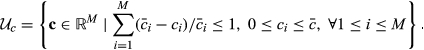

U_{c} = \{c \in R^{M} ∣ \sum_{i = 1}^{M} ({\bar{c}}_{i} - c_{i}) / {\bar{c}}_{i} \leq 1, 0 \leq c_{i} \leq \bar{c}, \forall 1 \leq i \leq M\} .

For demand uncertainty, the demand uncertainty set follows the structure defined in section 2.3:

\begin{matrix} U_{d} = & \{d \in R^{N} ∣ \sum_{j = 1}^{N} (d_{j} - {\bar{d}}_{j}) \leq γ, \sum_{j = 1}^{N} \frac{| d_{j} - {\bar{d}}_{j} |}{σ_{j}} \leq β, \\ | d_{j} - {\bar{d}}_{j} | \leq α σ_{j}, \forall 1 \leq j \leq N\} \end{matrix}

with parameters

σ_{j} = 0.15 {\bar{d}}_{j}, α = 2

, β = 8,

γ = 0.5 \sum_{j = 1}^{N} σ_{j}

. Under these assumptions, we solve the TTS model (11) for GM's network. Note that the TTS model requires that all of the demand in

U_{d}

to be filled during TTS. This is more conservative than the SG model we studied numerically in section 4, because in section 4, we allow 5% of the total demand to be lost. Following the discussion from section 2.1, we can also relax the conservativeness by shrinking the uncertainty set. For example, if we let

U_{d}^{'} = 0.95 \cdot U_{d}

, the TTS under

U_{d}^{'}

corresponds to firm requiring that 95% of demand for each product to be filled during TTS.

Tables 6 and 7 list the TTS of GM's network under different flexibility designs given inventory budget R (measured in weeks of demand) with demand uncertainty set

U_{d}

(100% fill rate) and

U_{d}^{'}

(95% fill rate per product), respectively. To populate Tables 6 and 7, the TTS under each flexibility design only needs to be computed for R = 1, as the TTS under the same flexibility design with R = x can be obtained by multiplying the TTS with R = 1 by a factor of x for any positive x. Once the TTS under a flexibility structure is computed with R = 1 (one week of extra inventory), the firm can use it to consider how much extra inventory is needed to protect its supply chain against disruptions. For example, under the base design with no flexibility (see Figure 3), if GM wants to maintain 100% of its demand with one week of extra inventory, its TTS is about 0.91 week; and this number would increase threefold if GM is willing to hold 3 weeks of inventory.

Table 6

TTS Achieved under Different Inventory Budget and

U_{d}

	Base	2‐chain	3‐chain	4‐chain	Full
R = 1 (week)	0.91	2.00	3.10	3.43	3.77
R = 2 (weeks)	1.82	4.00	6.21	6.86	7.54
R = 3 (weeks)	2.73	6.00	9.31	10.29	11.30

Table 7

TTS Achieved under Different Inventory Budget and

U_{d}^{'}

	Base	2‐chain	3‐chain	4‐chain	Full
R = 1 (week)	0.96	2.19	3.76	4.22	4.54
R = 2 (weeks)	1.92	4.38	7.52	8.44	9.08
R = 3 (weeks)	2.89	6.57	11.27	12.66	13.62

From Tables 6 and 7, we observe that adding partial flexibility to the system can greatly increase TTS of a supply chain. Under 3‐chain, the TTS with 100% fill rate and R = 1 is greater than 3 weeks, so GM's supply chain is robust against any disruption less than three weeks with one week of inventory. If GM sets its service level to just 95% for each product, under 3‐chain, the TTS is further increased to 3.76 weeks with R = 1. Under this circumstance, GM can hedge against disruption for over 11 weeks (almost three months) with just three weeks of inventory.

Cost Minimization Model

Sometimes, a supply chain manager does not set a particular service guarantee level, but would rather include the service level as a part of overall cost. In this case, the problem of cost minimization facing demand and capacity uncertainties can also be formulated as a two‐stage robust optimization problem, which we call the cost minimization (CM) model. Like the service guarantee model, the firm determines the inventory level for each product in the first stage; in the second stage, the firm minimizes the cost based on the realized product demand and available plant capacities.

The total cost in the CM model may include inventory, production, underage (lost sales) and overage costs. For product j, we denote the unit inventory holding cost to be h _j, the unit underage (lost sales) cost to be u _j, and the unit overage (excess inventory) cost to be o _j. The unit product cost of product j at plant i is denoted by f _ij. We define

Π (F, s, c, d)

to be the second stage cost, given flexibility design

F

, inventory vector s = (s ₁, s ₂, …, s _N) (decision from the first stage), and realized capacities c and demands d. We introduce a new decision variable, η, to represent the second stage cost. The CM model can be then formulated as follows.

\begin{matrix} (CM) min_{s, η} & \sum_{j = 1}^{N} h_{j} s_{j} + η \\ s.t. & Π (F, s, c, d) \leq η, \forall (c, d) \in U, \\ s \in X_{s}, η \in X_{η}, \end{matrix}

(12)

where

\begin{matrix} Π (F, s, c, d) & = min_{l, x} \sum_{(S_{i}, T_{j}) \in F} f_{ij} x_{ij} + \sum_{j = 1}^{N} u_{j} l_{j} + \sum_{j = 1}^{N} o_{j} {(s_{j} - d_{j})}^{+} \\ s.t. & \sum_{i : (S_{i}, T_{j}) \in F} x_{ij} + l_{j} \geq d_{j} - s_{j}, \forall 1 \leq j \leq N, \\ \sum_{j : (S_{i}, T_{j}) \in F} x_{ij} \leq c_{i}, \forall 1 \leq i \leq M, l_{j}, x_{ij} \geq 0 . \end{matrix}

(13)

In the last constraint of equation 12, X _s and X _η are polyhedral sets representing constraints on inventory decisions and second stage cost, respectively. Like the SG model, x _ij(c, d) denotes the production of product j by plant i, and l _j(c, d) denotes the lost sales of product j. To keep notations succinct, we use x _ij and l _j instead in formulation 13. As it turns out, the constraint generation algorithm we described in section 2.2 can be also applied to the cost minimization (CM) model.

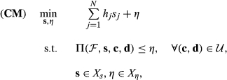
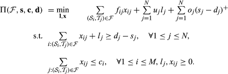
We note that the cost minimization (CM) model is a generalization of the service guarantee (SG) model. More specifically, for the CM model, if we set o _j = 0, f _ij = 0, u _j = 1 for all i, j, and X _η = {η¦η = δ}, then we recover the SG model. Because of its generality, the CM model can be applied to many different problems. While the CM model is more general, the more specialized structure in the SG model makes it much easier to solve numerically, and allows us to incorporate additional features such as TTS (section 5.1) and multi‐stage supply chains (section 5.3). Moreover, the simplicity of the SG model can be advantageous; in some situations, it is difficult to accurately estimate the costs of lost sales due to its long term effect (Latour 2001).

Multi‐Stage Service Guarantee Model

In section 2.1, we showed that if the firm specifies a service guarantee for each individual product, the problem can be reduced to a special case of the SG model by setting δ = 0 and modifying the demand uncertainty set. In this subsection, we show that the SG model can be extended for a multi‐stage supply chain when δ = 0.

Suppose there are K stages in the supply chain. For all k = 1, …, K, stage k consists of M ^k plants/suppliers, and

N^{k}

products/components. The stage indices are counted backward, so the final products are produced in stage 1, and the products/components in stage k require components from stage k + 1. Furthermore, we assume the bill of material information at stage k is represented by a matrix A ^k, such that one unit of product j at stage k requires

A_{j^{'} j}^{k}

units of component

j^{'}

at stage k + 1.

Let

s_{j}^{k}

be the inventory of product j at stage k, with unit holding cost

h_{j}^{k}

. Let

\tilde{Π} (F, s, c, d)

be the total lost sales for the final products given inventory s, capacity c and demand of final products d. The multi‐stage service guarantee (m‐SG) model can be formulated as

\begin{matrix} (m - SG) min & \sum_{k = 1}^{K} \sum_{j = 1}^{N^{k}} h_{j}^{k} s_{j}^{k} \\ s.t. & \tilde{Π} (F, s, c, d) \leq 0, \forall (c, d) \in U \\ s_{j}^{k} \geq 0, \end{matrix}

where

\begin{matrix} \tilde{Π} (F, s, c, d) & = min \sum_{j = 1}^{N^{1}} l_{j} \\ s.t. & \sum_{i : (S_{i}^{1}, T_{j}^{1}) \in F} x_{ij}^{1} + l_{j} \geq d_{j} - s_{j}^{1}, \forall 1 \leq j \leq N^{1} \\ \sum_{i : (S_{i}^{k + 1}, T_{j^{'}}^{k + 1}) \in F} x_{i j^{'}}^{k + 1} + s_{j^{'}}^{k + 1} \\ \geq \sum_{j = 1}^{N^{k}} A_{j^{'} j}^{k} \sum_{i : (S_{i}^{k}, T_{j}^{k}) \in F} x_{ij}^{k}, \forall 1 \leq k \leq K - 1 \\ \sum_{j : (S_{i}, T_{j}) \in F} x_{ij}^{k} \leq c_{i}^{k}, \forall 1 \leq k \leq K, 1 \leq i \leq M^{k} \\ l_{j}, x_{ij}^{k} \geq 0 . \end{matrix}

In the subproblem

\tilde{Π} (F, s, c, d)

, the first set of constraints defines the lost sales of final products. The second set of constraints ensures that there are enough components at stage k + 1 to satisfy production at stage k. The third set of constraints enforces capacity limits.

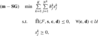
The m‐SG model can also be solved efficiently using constraint generation algorithm (Wang 2016). To apply constraint generation, we can first decompose the subproblems for different stages, using the fact that the lost sales allowance δ is zero and making affine transformation on the uncertainty sets. To this end, we define uncertainty sets

U^{1} = U

, and

U^{k + 1} = {(c, A^{k} d^{k}) | (c, d^{k}) \in U^{k}}

for all k = 1, …, K − 1. Let

{\tilde{Π}}^{k} (F, s, c, d^{k})

be the lost sales of stage k, we have

\begin{matrix} ({m - SG}^{'}) & min \sum_{k = 1}^{K} \sum_{j = 1}^{N^{k}} h_{j}^{k} s_{j}^{k} \\ s.t. & {\tilde{Π}}^{k} (F, s, c, d^{k}) \leq 0, \forall (c, d^{k}) \in U^{k}, k = 1, \dots, K \\ s_{j}^{k} \geq 0, \end{matrix}

where

\begin{matrix} {\tilde{Π}}^{k} (F, s, c, d^{k}) & = min \sum_{j = 1}^{N^{k}} l_{j} \\ s.t. & \sum_{i : (S_{i}^{k}, T_{j}^{k}) \in F} x_{ij}^{k} + l_{j} \geq d_{j}^{k} - s_{j}^{k}, \forall 1 \leq j \leq N^{k} \\ \sum_{j : (S_{i}, T_{j}) \in F} x_{ij}^{k} \leq c_{i}^{k}, \forall 1 \leq i \leq M^{k} \\ l_{j}, x_{ij}^{k} \geq 0 . \end{matrix}

We note that for the general case of the SG model with δ > 0, this reformulation technique does not work because the subproblem cannot be decomposed for different stages. Nevertheless, even when δ is fixed to zero, the firm can still adjust its target service guarantee by using different demand uncertainty sets (see section 2.1).

Conclusion

We consider a firm that coordinates process flexibility and inventory decisions to mitigate supply risk. The interplay of process flexibility and inventory is modeled as a two‐stage robust optimization problem, which can be solved efficiently using constraint generation algorithm. Under some symmetry assumptions, the solution of the robust optimization model can be characterized, allowing us to better understand the change in optimal inventory as flexibility or capacity uncertainty changes. Using the characterization, we find that the widely used 2‐chain structure does not provide enough protection against supply disruption. Moreover, we show that the optimal inventory decision critically depends on the flexibility design of the supply network. In particular, there tend to be a shift of inventories from high variability products to low variability products as the degree of process flexibility increases. We refer to such phenomenon as the flipping effect, which is demonstrated using both theoretical analysis and numerical experiments.

Our robust optimization model is applicable to various types of risk mitigation problems, as the model can be extended to incorporate different underage, overage, and inventory costs. The model can be also extended to incorporate multi‐stage supply chain and unknown disruption time. In the numerical experiment, we apply the robust optimization method to a risk mitigation example in an automotive supply chain. This application demonstrates that our model can be an effective tool for analyzing the hybrid risk mitigation strategy that combines process flexibility and inventory.

References

Arreola‐Risa

DeCroix

. 1998. Inventory management under random supply disruptions and partial backorders. Nav. Res. Logisti. 45(7): 687–703.

Atamtürk

Zhang

. 2007. Two‐stage robust network flow and design under demand uncertainty. Oper. Res. 55(4): 662–673.

Bandi

Bertsimas

. 2012. Tractable stochastic analysis in high dimensions via robust optimization. Math. Programm. 134(1): 23–70.

Bassamboo

Randhawa

R. S.

Mieghem

J. A. V.

. 2012. A little flexibility is all you need: On the asymptotic value of flexible capacity in parallel queuing systems. Oper. Res. 60(6): 1423–1435.

Bassamboo

Randhawa

R. S.

Van Mieghem

J. A.

. 2010. Optimal flexibility configurations in newsvendor networks: Going beyond chaining and pairing. Management Sci. 56(8): 1285–1303.

Ben‐Tal

El Ghaoui

Nemirovski

. 2009. Robust Optimization, Princeton University Press, New Jersey, USA.

Ben‐Tal

Goryashko

Guslitzer

Nemirovski

. 2004. Adjustable robust solutions of uncertain linear programs. Math. Program. 99(2): 351–376.

Bertsimas

Brown

Caramanis

. 2011. Theory and applications of robust optimization. SIAM Rev. 53(3): 464–501.

Bertsimas

Thiele

. 2006. A robust optimization approach to inventory theory. Oper. Res. 54(1): 150–168.

10.

Bertsimas

Tsitsiklis

. 1997. Introduction to Linear Optimization, Athena Scientific, Belmont, MA.

11.

Bish

Wang

. 2004. Optimal investment strategies for flexible resources, considering pricing and correlated demands. Oper. Res. 52(6): 954–964.

12.

Bollapragada

Rao

U. S.

Zhang

. 2004. Managing inventory and supply performance in assembly systems with random supply capacity and demand. Management Sci. 50(12): 1729–1743.

13.

Bonami

Kilinç

Linderoth

. 2012. Algorithms and software for convex mixed integer nonlinear programs. Lee

Leyffer

, eds. Mixed Integer Nonlinear Programming. Springer, Berlin, 1–39.

14.

Chopra

Sodhi

M. S.

. 2014. Reducing the risk of supply chain disruptions. MIT Sloan Manag. Rev. 55(3): 73.

15.

Chou

Teo

C.‐P.

Zheng

. 2011. Process flexibility revisited: The graph expander and its applications. Oper. Res. 59(5): 1090–1105.

16.

Chou

M. C.

Chua

G. A.

Teo

C.‐P.

Zheng

. 2010. Design for process flexibility: Efficiency of the long chain and sparse structure. Oper. Res. 58(1): 43–58.

17.

Chou

M. C.

Chua

G. A.

Zheng

. 2014. On the performance of sparse process structures in partial postponement production systems. Oper. Res. 62(2): 348–365.

18.

Culp

. 2013. Supply chain disruption a major threat to business. Forbes. Published on Feburary 15, 2013.

19.

DeCroix

G. A.

2013. Inventory management for an assembly system subject to supply disruptions. Management Sci. 59(9): 2079–2092.

20.

Dyer

Stougie

, 2006. Computational complexity of stochastic programming problems. Math. Program. 106(3): 423–432.

21.

Fine

C. H.

Freund

R. M.

. 1990. Optimal investment in product‐flexible manufacturing capacity. Management Sci. 36(4): 449–466.

22.

Fisher

Raman

. 1996. Reducing the cost of demand uncertainty through accurate response to early sales. Oper. Res. 44(1): 87–99.

23.

Gabrel

Murat

Thiele

. 2014. Recent advances in robust optimization: An overview. Eur. J. Oper. Res. 235(3): 471–483.

24.

Graves

S. C.

Willems

S. P.

. 2000. Optimizing strategic safety stock placement in supply chains. Manuf. Serv. Oper. Manag. 2(1): 68–83.

25.

Gürler

Ü.

Parlar

. 1997. An inventory problem with two randomly available suppliers. Oper. Res. 45(6): 904–918.

26.

Hopp

Iravani

Liu

. 2012. Mitigating the impact of disruptions in supply chains. Gurnani

Mehrotra

Ray

, eds. Supply Chain Disruptions. Springer, London, 21–49.

27.

Hopp

W. J.

Tekin

Van Oyen

M. P.

. 2004. Benefits of skill chaining in serial production lines with cross‐trained workers. Management Sci. 50(1): 83–98.

28.

Jansen

2017. Delta outage a reminder of fragility of airline computers. USA TODAY. Published on January 30, 2017.

29.

Jordan

W. C.

Graves

S. C.

. 1995. Principles on the benefits of manufacturing process flexibility. Management Sci. 41(4): 577–594.

30.

Kim

C.‐R. K.

2011. Toyota aims for quake‐proof supply chain. Reuters. September 6, 2011.

31.

Latour

2001. Trial by fire: A blaze in albuquerque sets off major crisis for cell‐phone giants. The Wall Street Journal. Published on January 29, 2011.

32.

Meyer

R. R.

Rothkopf

M. H.

Smith

S. A.

. 1979. Reliability and inventory in a production‐storage system. Management Sci. 25(8): 799–807.

33.

O’Marah

2017. Supply chain risk 2020: New worries. Forbes. Published on October 6, 2017.

34.

Shapiro

Nemirovski

. 2005. On complexity of stochastic programming problems. Jeyakumar

Rubinov

, eds. Continuous Optimization. Springer, Berlin, 111–146.

35.

Simchi‐Levi

2010. Operations Rules: Delivering Customer Value through Flexible Operations, The MIT Press, Cambridge, MA.

36.

Simchi‐Levi

Schmidt

Wei

. 2014. From superstorms to factory fires: Managing unpredictable supply chain disruptions. Harv. Bus. Rev. 92(1–2): 96–101.

37.

Simchi‐Levi

Schmidt

Wei

Zhang

P. Y.

Combs

Gusikhin

Sander

Zhang

. 2015. Identifying risks and mitigating disruptions in the automotive supply chain. Interfaces 45(5): 375–390.

38.

Simchi‐Levi

Wei

. 2012. Understanding the performance of the long chain and sparse designs in process flexibility. Oper. Res. 60(5): 1125–1141.

39.

Sodhi

M. S.

Tang

C. S.

. 2012. Strategic approaches for mitigating supply chain risks. Hillier

F. S.

, ed. Managing Supply Chain Risk, volume 172 of International Series in Operations Research and Management Science. Springer, New York, 95–108.

40.

Song

J.‐S.

Zipkin

P. H.

. 1996. Inventory control with information about supply conditions. Management Sci. 42(10): 1409–1419.

41.

Swaminathan

J. M.

Tayur

S. R.

. 1998. Managing broader product lines through delayed differentiation using vanilla boxes. Management Sci. 44(12‐part‐2): S161–S172.

42.

Tang

Tomlin

. 2008. The power of flexibility for mitigating supply chain risks. Int. J. Prod. Econ. 116(1): 12–27.

43.

Thiele

Terry

Epelman

. 2010. Robust linear optimization with recourse. University of Michigan, IOE Technical Report TR09‐01.

44.

Tomlin

2006. On the value of mitigation and contingency strategies for managing supply chain disruption risks. Management Sci. 52(5), 639–657.

45.

Tomlin

Wang

. 2005. On the value of mix flexibility and dual sourcing in unreliable newsvendor networks. Manuf. Serv. Oper. Manag. 7(1): 37–57.

46.

Wang

2016. Dynamic learning and optimization for operations management problems. PhD thesis, Massachusetts Institute of Technology.

47.

Wang

Zhang

. 2015. Process flexibility: A distribution‐free bound on the performance of k‐chain. Oper. Res. 63(3): 555–571.

48.

Zeng

Zhao

. 2013. Solving two‐stage robust optimization problems using a column‐and‐constraint generation method. Oper. Res. Lett. 41(5): 457–461.