Process Flexibility Analysis for Production Systems with Differentiated Margins Under Supply Risk

Abstract

To mitigate supply and demand uncertainties, firms often design highly flexible production networks. This study investigates process flexibility in production systems subject to supply disruptions and stochastic demands with differentiated profit margins. In particular, we model supply disruptions as failures of arcs in the network, with node-based disruptions treated as a special case in which all arcs connected to a node simultaneously fail. To address the cost implications of such disruptions, we investigate the design of process flexibility under a robust optimization framework. We first develop a greedy algorithm under deterministic demand to efficiently evaluate the worst-case disruption scenario, and demonstrate the significant advantage of the alternate long-chain design under such disruptions. Subsequently, under stochastic demand, by introducing the marginal profit group index under disruption (MPGID), we characterize the worst-case total profit as a function of both the flexibility design and demand uncertainty, modeled through a partwise independently symmetric perturbation set. This representation enables direct performance comparisons across different flexibility configurations under disruption risk. For the case involving two products with distinct profit margins under supply disruption risk, we demonstrate that the alternate long-chain design outperforms all other long-chain configurations in terms of worst-case profitability. In addition, in certain cases, arc-based disruptions can be just as devastating as plant-node disruptions, particularly when they lead to the loss of high-margin demand. However, our fragility analysis reveals that this design becomes increasingly vulnerable as disruption risks intensify. To address this issue, we propose an MPGID-based heuristic that systematically generates flexible designs to mitigate both supply and demand uncertainties.

Keywords

Process Flexibility Differentiated Margins Supply Disruption Robust Optimization

1. Introduction

In today’s globalized business environment, manufacturing firms increasingly face the severe challenges of supply disruptions, even as production efficiency continues to advance. The expansion of transnational corporations and overseas manufacturing operations—such as Apple, Tesla, and Admiral Overseas Corporation (AOC)—has extended supply chains across broader geographic regions, significantly increasing their complexity and vulnerability. Consequently, firms are now more frequently exposed to high-impact disruptions that threaten the continuity of routine operations. For instance, supply chain managers at AOC have reported recurrent disruptions in recent years. These include the Red Sea crisis, which rendered major maritime shipping routes inoperative, the sustained low water levels in the Amazon region, which impaired inland transportation, and evolving international tariff policies, which have undermined inter-firm connectivity across multiple tiers. Such disruptions, often occurring along specific transportation arcs, highlight the fragility of extended supply networks. A particularly salient example is the 2011 earthquake in Japan, which brought the country’s manufacturing sector to a standstill and triggered cascading global supply chain disruptions across industries, including automotive, semiconductors, and electronics (Malcolm and Malcolm, 2011). These real-world events underscore the critical need to explicitly model transportation-arc-based disruptions in the design of robust process flexibility systems. In addition, disruptions can also arise from deliberate human interventions, terrorism, and social instability. For instance, in 2021, the grounding of a cargo ship in the Suez Canal resulted in massive delays to goods and introduced instability and trade disruptions globally (Harper, 2021). In particular, according to a survey, supply chain disruptions can cause an average annual loss of $182 million (Interos, 2022), and (Hendricks and Singhal, 2005) have shown that such disruptions could lead to a long-term decrease in stock returns (about 33%–40%).

In previous research, a variety of strategies have been proposed to safeguard firms against losses stemming from supply disruptions, including commercial insurance, multisourcing, and inventory reserves (Dong and Tomlin, 2012; Schmitt and Tomlin, 2012; Snyder et al., 2016). Among these, the design of process flexibility has emerged as a particularly effective approach to mitigate disruption-induced losses and enhance supply-demand coordination. As defined by Jordan and Graves (1995), process flexibility refers to a firm’s operational agility to produce a broad range of products within a single manufacturing system. Intuitively, flexible production resources can serve multiple product markets. Thus, when a supplier experiences a disruption, alternative flexible suppliers can compensate by fulfilling the affected demand. For instance, according to the Review of Maritime Transport 2020 published by the United Nations Conference on Trade and Development (UNCTAD), transportation and logistics restrictions, coupled with labor shortages during the coronavirus disease 2019 pandemic, severely delayed the delivery of components from China and other countries to manufacturing hubs in Southeast Asia (UNCTAD, 2020). Consequently, many firms were compelled to implement flexible contingency strategies, such as shifting from ground transportation to air freight or dynamically rerouting maritime shipments to alternative ports, underscoring the practical importance of flexibility in navigating large-scale supply disruptions.

In addition, during supply disruptions or limited production capacity, firms often face a practical necessity to prioritize certain products rather than supplying the full product mix. In such cases, differentiated profit margins naturally become a key driver of allocation decisions. For instance, during the global semiconductor shortage, many wafer foundries prioritized high-margin consumer electronics over lower-margin automotive chips (Piers, 2021). Apple, in its resource allocation strategy, concentrated capacity on its most profitable product lines, while reducing production for lower-margin segments. Similarly, Advanced Micro Devices (AMD) strategically focused on selling its most profitable chips, while ceding lower-end market segments to competitors such as Intel (Stephen and Subrat, 2021). These real-world practices underscore a crucial limitation of most existing process flexibility studies: They implicitly assume homogeneous products with identical profit margins, while in practice, product portfolios often exhibit substantial profit heterogeneity. Moreover, effective flexibility design must simultaneously account for product flexibility, capacity flexibility, and manufacture flexibility, each contributing differently to the system’s profit potential. Without sufficient flexibility across these dimensions, firms lack the agility to dynamically reallocate resources toward higher-margin opportunities when disruptions occur. Despite its growing practical relevance, most of the existing literature on process flexibility continues to assume homogeneous products with identical profit margins and focuses primarily on demand-side uncertainty. While recent studies have started to incorporate supply disruption risks in flexibility design for homogeneous product systems (e.g., Chen et al., 2025; Mehmanchi et al., 2021), the interaction between differentiated product margins and supply disruptions remains largely underexplored. To the best of our knowledge, Wang et al. (2022) is the only existing study that explicitly examines process flexibility design under differentiated profit margins. By focusing on deterministic supply conditions, it lays a foundation for future work that integrates margin differentiation with supply-side uncertainty—an important direction given the real-world practices of prioritizing high-margin products under disruptions.

In this paper, we analyze process flexibility design under the joint presence of differentiated profit margins and supply disruption risk. The main contributions of this study are summarized as follows.

First, we develop a greedy algorithm to evaluate the worst-case impact of arc-based disruptions under deterministic demand. Our analysis reveals that the alternate long-chain design provides clear advantages in enhancing capacity utilization and mitigating supply risks associated with arc failures, and it not only mitigates demand variability across heterogeneous products, but also proves highly effective against stochastic supply disruptions.

Then, when both supply disruptions and demand uncertainty are present, we formulate a maximum-flow profit model and employ duality theory to establish a mixed-integer linear program (MILP) framework, termed the marginal profit group index under disruption (MPGID). This formulation enables robust performance evaluation of flexibility designs. In particular, we show that the MPGID value induces a partial ordering of flexibility designs with respect to their worst-case profit performance under uncertainty.

In addition, focusing on a two-product system, we demonstrate that the alternate long-chain design consistently outperforms general long-chain designs across both arc-based and node-based disruptions. This finding extends the results of Wang et al. (2022) by incorporating supply-side risks, thereby enhancing the practical relevance of the alternate long-chain design. Contrary to intuition, our analysis indicates that, under specific conditions, localized arc-based disruptions may have consequences comparable to those of plant-node disruptions, especially when they selectively affect high-margin demands. Moreover, we identify that while the alternate long chain ( $A L$ ) offers strong robustness at moderate disruption levels, its fragility increases once disruption severity crosses a critical threshold.

Finally, we develop an MPGID-based heuristic algorithm to generate robust flexibility designs under differentiated profit margins and supply disruptions. To evaluate its effectiveness, we benchmark this heuristic against several existing approaches, including: (i) The DMGI heuristic from Wang et al. (2022), which considers differentiated margins without disruptions; (ii) the PCID heuristic of Mehmanchi et al. (2021), which addresses supply disruptions in homogeneous product systems; (iii) a Sample Average Approximation (SAA) method for jointly handling demand and disruption randomness; and (iv) the Expander heuristic from Chou et al. (2011), which focuses on demand means and production capacities under deterministic settings. Numerical experiments demonstrate that our MPGID-based heuristic exhibits superior robustness in most disruption scenarios, validating its practical applicability.

The remainder of this paper is organized as follows. Section 2 reviews the related literature and highlights the limitations of existing studies on flexibility design and network disruption analysis. In Section 3, we first demonstrate the effectiveness of the design $A L$ under deterministic demand with disruptions, introduce the MPGID model for scenarios involving both disruption and demand uncertainty, and derive the corresponding robust performance measures. Section 4 investigates the properties of the design $A L$ under the worst case of supply disruptions. Section 5 presents a heuristic algorithm for generating flexible designs and evaluates its performance through comprehensive numerical experiments. Finally, Section 6 concludes the paper by summarizing the key findings, discussing limitations, and outlining directions for future research. All technical proofs are provided in the Appendix.

2. Literature Review

This study is closely related to two major streams of literature, that is, the design of process flexibility and supply chain management under disruption risk.

Within the first stream, the seminal work by Jordan and Graves (1995) highlighted the operational benefits of long-chain designs based on empirical insights from General Motors, introducing the influential “chaining” heuristic to guide flexibility design. This motivated a substantial body of subsequent research to formalize and validate the principles of process flexibility design. Then, under the assumption of independent and identically distributed ( $i . i . d .$ ) product demands, Chou et al. (2010) offered a theoretical foundation by analyzing the asymptotic performance of long chains in large systems. Simchi-Levi and Wei (2012) extended this line of inquiry by focusing on 2-flexibility designs—where each node is connected to exactly two others—and demonstrated the dominance of long chains in such settings. Their work further revealed an increasing marginal value of each added arc when transitioning from a dedicated system toward a long-chain structure. To quantify the minimal structure required for near-complete flexibility, Chen et al. (2015) introduced the notion of probabilistic expanders and identified conditions under which a sparse network can still achieve near-optimal performance. Desir et al. (2016) showed that among all connected structures with a fixed number of arcs, the long chain consistently yields superior performance. More recently, Wang et al. (2022) made significant progress by extending flexibility theory to systems with differentiated product margins—a setting more aligned with real-world practices. They proposed an MILP model to evaluate the robust performance of flexibility designs and demonstrated that the $A L$ —where each supply node connects to two product nodes with differing profit margins—outperforms all other long-chain configurations in such settings.

Nevertheless, several studies have also highlighted the limitations of long-chain designs. In particular, Chou et al. (2008) showed that as the coefficient of variation in demand increases, the performance gap between long chains and fully flexible designs becomes more significant. To enhance flexibility, Aksin and Karaesmen (2007) extended the long-chain concept and proposed the “ $K$ -chain” design, in which each product can be produced by $K$ plants and each plant can manufacture $K$ products. Later, Wang and Zhang (2015) derived a distribution-free bound on expected sales and demonstrated that a 6-chain configuration could achieve up to 90% of the efficiency of full flexibility under demand uncertainty. Zhong et al. (2025) further extended this result to settings with supply uncertainty. These findings have spurred a growing interest in the design of sparse yet effective flexible networks. For example, Mak and Shen (2009) incorporated differential pricing and cost structures into a stochastic optimization framework for flexibility design. Building on this, Feng et al. (2017) proposed an SAA-based heuristic to solve their enhanced model. In the context of multiperiod fulfillment, Shi et al. (2019) introduced the concept of the generalized chaining gap and proved that, in capacity-constrained systems, a sparse flexibility structure with $m + n$ links is sufficient to achieve full capacity utilization. This line of work was further extended by Xu et al. (2020) to encompass more general asymmetric systems. More recently, DeValve et al. (2023) employed submodular optimization to establish a unified framework that provides performance guaranties for a range of flexibility design algorithms. For a comprehensive survey on this topic, readers are referred to Wang et al. (2021).

Differing from prior research, this paper advances the study of process flexibility design by simultaneously considering heterogeneous marginal contributions and the presence of supply disruptions in both nodes and arcs—an area that has received limited attention in the literature. Notably, Wang et al. (2022) is the only study to explicitly examine process flexibility with differentiated profit margins without considering the risk of supply disruptions. Building upon and extending this work, we demonstrate that the optimality of $A L$ persists even under disruption risks, and we analyze their fragility when disruption severity increases. Furthermore, we develop a heuristic algorithm capable of generating flexible network designs in general multiproduct systems subject to disruptions. Our numerical experiments show that this algorithm outperforms existing approaches, providing a robust and practically relevant method for designing flexible production systems in disruption-prone environments.

Another stream of literature focuses on mitigating supply disruption risks through operational strategies. In particular, numerous studies in vertical supply chains have examined the role of inventory as a buffer against such disruptions. For example, Tomlin (2006) provided foundational insights into multisourcing under risk, while Ruiz-Torres and Mahmoodi (2007) further analyzed supplier selection strategies in disruption-prone environments. More recently, Wu et al. (2023) studied decentralized inventory positioning strategies. Other approaches included the use of business interruption insurance mechanisms (Dong and Tomlin, 2012) and the application of digital twin frameworks to support inventory and cash flow management during disruptions (Badakhshan and Ball, 2023).

In the context of supply chain network design under disruption risks, An et al. (2014) introduced a two-stage robust optimization framework for designing resilient $p$ -median facility location networks capable of withstanding disruptions. Subsequently, Simchi-Levi et al. (2015) proposed an innovative risk exposure model that quantified the impact of various disruptions by integrating recovery time and service time. Shen et al. (2021) studied a reliable hub location model that assigned both primary and backup paths for each origin-destination pair to mitigate transportation risks from random disruptions. More recently, Vidza et al. (2025) proposed a comprehensive decision-making framework that combines topological and operational metrics to simulate node-based disruptions and optimize network structures, while Jin and Vergara (2025) formulated an optimization model for selecting critical nodes and mitigation strategies within budget constraints to improve network robustness.

However, only a few studies have examined the design of process flexibility as a means of mitigating the negative impacts of disruption risk. Recently, Rujeerapaiboon et al. (2023) demonstrated that despite the possibility of node-based disruptions, the long chain remained a feasible option to replace full flexibility. Chen et al. (2025) found that as disruption risk increased, the long chain exhibited better performance when supply resources were aligned with average demand. While these studies primarily focused on disruptions at supply nodes, they largely overlooked disruptions in the arcs of the network. In practice, arc-based disruptions could significantly affect the feasibility and effectiveness of flexibility configurations. To the best of our knowledge, only one paper, Mehmanchi et al. (2021), incorporated chance constraints to model both node-based and arc-based disruptions and analyzed the structural properties of long-chain flexibility designs in systems with homogeneous products under supply disruptions. Unlike previous research, we incorporate differentiated profit margins and optimize supply-demand connections under disruption scenarios through process flexibility design, aiming to mitigate losses caused by arc-based disruptions in supply chain networks.

3. Problem Formulation

We model the process flexibility design of a production system as a maximum flow network, where production capacities are allocated across multiple products based on a specified flexibility configuration. The system manufactures heterogeneous products with differentiated profit margins. At the same time, production plants are subject to disruption risks that may materialize at two levels: (i) The plant-product level, where individual arcs representing plant-to-product capabilities are rendered inoperative; and (ii) the plant level, where all associated arcs of a given plant are simultaneously disrupted, resulting in complete production outages. For ease of analysis, we consider a single-period demand setting. Throughout the model, we use $[n] = {1, 2, \dots, n}$ to denote the index set of size $n$ . Boldface symbols such as $x \in R^{n}$ represent vectors, with $x_{i}$ denoting the $i$ th component of vector $x$ for all $i \in [n]$ . For a vector $x \in R^{n}$ , denote ${min}^{i} (x)$ as the $i$ th smallest element in the set $(x_{1}, \dots, x_{n})$ . Network structures are denoted by script letters, such as $G$ for a given flexibility design, where $(a, b) \in G$ indicates that arc $(a, b)$ exists in design $G$ . The uncertainty set is denoted by $U$ , and $U_{1} \times U_{2}$ represents the Cartesian product of two uncertainty sets. Finally, $I {*}$ denotes an indicator function, which equals 1 if the stated condition “ $*$ ” holds and 0 otherwise.

3.1. Definition and Modeling

Consider a production system in which a set of products $B = {b_{j} | j \in [n]}$ is manufactured by a set of plants $A = {a_{i} | i \in [m]}$ . Notably, the cardinalities of sets $A$ and $B$ are not necessarily equal, allowing for both balanced and unbalanced network structures. Product demands follow a joint probability distribution, with partial moment information available (e.g., means and standard deviations). Let $d = (d_{1}, \dots, d_{n})$ denote a realization of demands, and $μ = (μ_{1}, \dots, μ_{n})$ represent the corresponding mean demand vector. Each plant $a_{i} \in A$ has a production capacity $c_{i}$ , and may allocate it to produce multiple units of any product $b_{j} \in B$ , where the unit profit is $p_{j}$ . Suppose there are $T$ distinct profit margin levels, with $p_{j} \in {P_{1}, \dots, P_{T}}$ for each $1 \leq j \leq n$ and $P_{1} < P_{2} < \dots < P_{T}$ . We define $V_{t}$ as the group of products sharing the profit margin $P_{t}$ , that is, $V_{t} = {b_{j} \in B | p_{j} = P_{t}}$ .

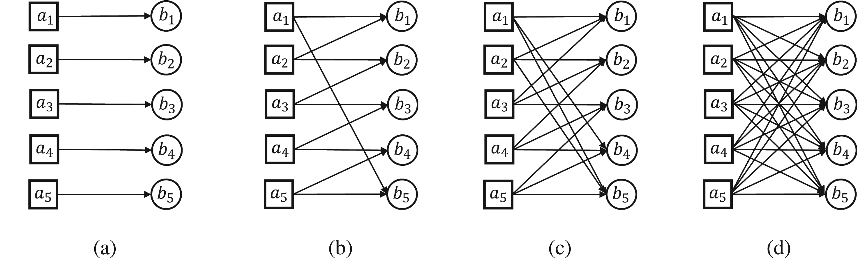
Let $G$ denote a given flexibility design, representing the network configuration between plants and products. An arc $(a_{i}, b_{j}) \in G$ exists if plant $a_{i}$ can produce product $b_{j}$ . The total number of arcs is denoted by $| G |$ . Several standard configurations for flexibility designs are widely studied in the literature:

Dedicated design: $D^{n} = {(a_{i}, b_{i}) ∣ i \in [n]}$ features a strict one-to-one mapping between plants and products, ensuring that each product is produced by exactly one unique plant.

Fully flexible design: $F^{n} = {(a_{i}, b_{j}) ∣ i, j \in [n]}$ allows every plant to produce every product, thus maximizing system flexibility.

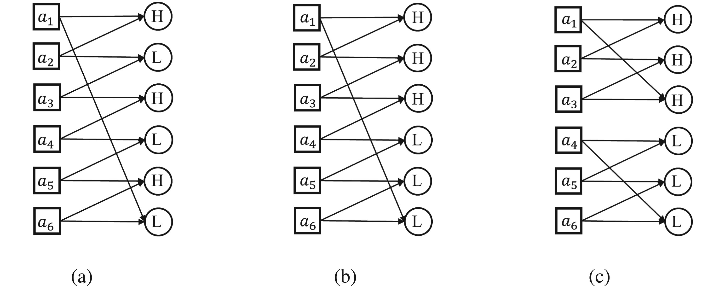
Long chain design: $L_{2}^{n} = D^{n} \cup {(a_{i}, b_{i - 1}) ∣ i \in [n]} \cup {(a_{1}, b_{n})}$ is a sparse yet effective configuration in which each product is connected to exactly two plants. This structure enables improved capacity utilization while maintaining a limited number of connections.

Figure 1 illustrates these configurations for the case where

n = 5

Figure 1.

Flexibility designs with $n = 5$ . (a) $D^{5}$ , (b) $L_{2}^{5}$ , (c) $L_{3}^{5}$ (3 chain) and (d) $F^{5}$ .

However, in supply-disrupted environments, each arc in the flexibility design $G$ —representing a specific plant-product production capability—may be subject to disruption. Arc-based disruptions are common in practice and occur across a wide range of operational contexts. Asghari et al. (2023) investigated path network designs under road congestion and disruption scenarios, further underscoring the relevance of arc-level risks in networked systems. In manufacturing contexts, disruptions often manifest as failures in specific plant-product links due to material shortages or supplier constraints, rather than complete plant shutdowns. For instance, one of our collaborators—AOC—may be unable to manufacture high-end gaming monitors when specific components, such as G-Sync or FreeSync chips, are unavailable, yet can continue producing standard monitors using more generic parts like LCD panels and controllers. These scenarios highlight a critical operational feature: Arc-based disruptions impair the configuration of production assignments, not necessarily the total capacity. Consequently, the ability to flexibly reallocate production across differentiated products becomes indispensable. Motivated by these real-world phenomena, this study investigates the design of process flexibility under arc-based disruption risks (with node-based disruption as a special case) within production networks, aiming to improve system resilience by ensuring production adaptability in the face of partial capacity constraints.

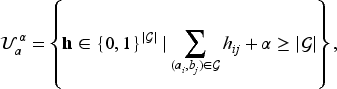
In particular, we introduce a binary random variable $h_{i j}$ to characterize the disruption state of arc $(a_{i}, b_{j})$ , where $h_{i j} = 0$ indicates that the arc is disrupted and $h_{i j} = 1$ indicates otherwise. Accordingly, denote $U_{a}^{α}$ as the symmetric uncertainty set for arc-based disruptions, allowing for a maximum of $α$ disrupted arcs. Formally, the Arc-based Disruption Uncertainty Set can be defined as

U_{a}^{α} = {h \in {0, 1}^{| G |} | \sum_{(a_{i}, b_{j}) \in G} h_{i j} + α \geq | G |},

where each

h

represents an instance of disruption, and

α \in Z^{+}

determines the budget for arc-based disruption risk.

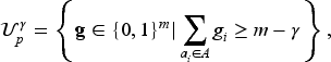
Another common type of disruption is the complete breakdown of a production facility, which typically results in a total loss of its production capacity. Such disruptions may arise from power outages, natural disasters, or other severe operational failures. For instance, Krishnamoorthy et al. (2014) reviewed how failures in public utilities (e.g., electricity or communication networks) and social disturbances (e.g., labor strikes or server outages) can severely affect service operations. In 2011, a magnitude 9.0 earthquake followed by a devastating tsunami hit northeastern Japan, forcing hundreds of manufacturing plants to shut down (Inajima and Okada, 2012). In addition, a cyberattack on the Colonial Pipeline network triggered widespread fuel shortages and temporarily disrupted airport operations across the U.S. East Coast (Josephs, 2021). We refer to this as a plant (node-based) disruption and introduce a corresponding uncertainty set, analogous to that used for arc-based disruptions. We define the Node-based Disruption Uncertainty Set $U_{p}^{γ}$ as a symmetric uncertainty set that captures scenarios involving node-based disruptions. Specifically, it allows for up to $γ$ plants to be disrupted simultaneously. The set $U_{p}^{γ}$ is characterized as follows:

U_{p}^{γ} = {g \in {0, 1}^{m} | \sum_{a_{i} \in A} g_{i} \geq m - γ},

where

g \in U_{p}^{γ}

denotes a realization of node-based disruption (

g_{i} = 1

indicates that plant

i

is operating normally, and

g_{i} = 0

indicates a disruption). For notational simplicity, we omit the parameters

α

(for arc-based disruptions) and

γ

(for node-based disruptions), and refer to the uncertainty sets as

U_{a}

and

U_{p}

, respectively.

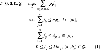
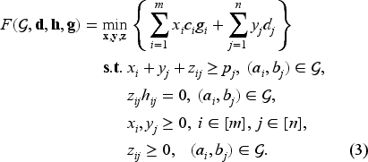
Given a flexibility design $G$ , a demand realization $d$ , and disruption realizations $h = {h_{i j}}$ and $g = {g_{i}}$ , the decision-maker’s problem is to determine the production volume (flow) $f_{i j}$ —that is, the amount of product $j$ produced at plant $i$ —to maximize the total profit $F (G, d, h, g)$ as follows.

\begin{aligned} F (G, d, h, g) = max_{f} & \sum_{(a_{i}, b_{j}) \in G} p_{j} f_{i j} \\ s . t . & \sum_{j = 1}^{n} f_{i j} \leq c_{i} g_{i}, i \in [m], \\ \sum_{i = 1}^{m} f_{i j} \leq d_{j}, j \in [n], \\ 0 \leq f_{i j} \leq M h_{i j}, (a_{i}, b_{j}) \in G . \end{aligned}

(1)

In Problem (1), the first constraint ensures that the total capacity utilized at plant

i

does not exceed its available capacity

c_{i}

. The second constraint guaranties that the total production quantity of product

j

does not surpass the realized demand

d_{j}

. The third constraint imposes a disruption-dependent restriction on the arc

(a_{i}, b_{j})

: If a disruption occurs (i.e.,

h_{i j} = 0

), then

f_{i j} = 0

; otherwise (

h_{i j} = 1

f_{i j}

is unrestricted, where

M

denotes a sufficiently large constant. This model evaluates the maximum total profit based on the production quantities of heterogeneous products, assuming the firm is a price taker—that is, marginal profits are fixed and independent of production quantities. This treatment effectively omits explicit cost considerations, thereby reducing the number of parameters in the model and simplifying the analysis. In the Appendix, we extend the discussion to include arc-specific production costs and demonstrate that the resulting structural properties remain largely consistent with the cost-agnostic formulation.

3.2. Analysis Under Deterministic Demand

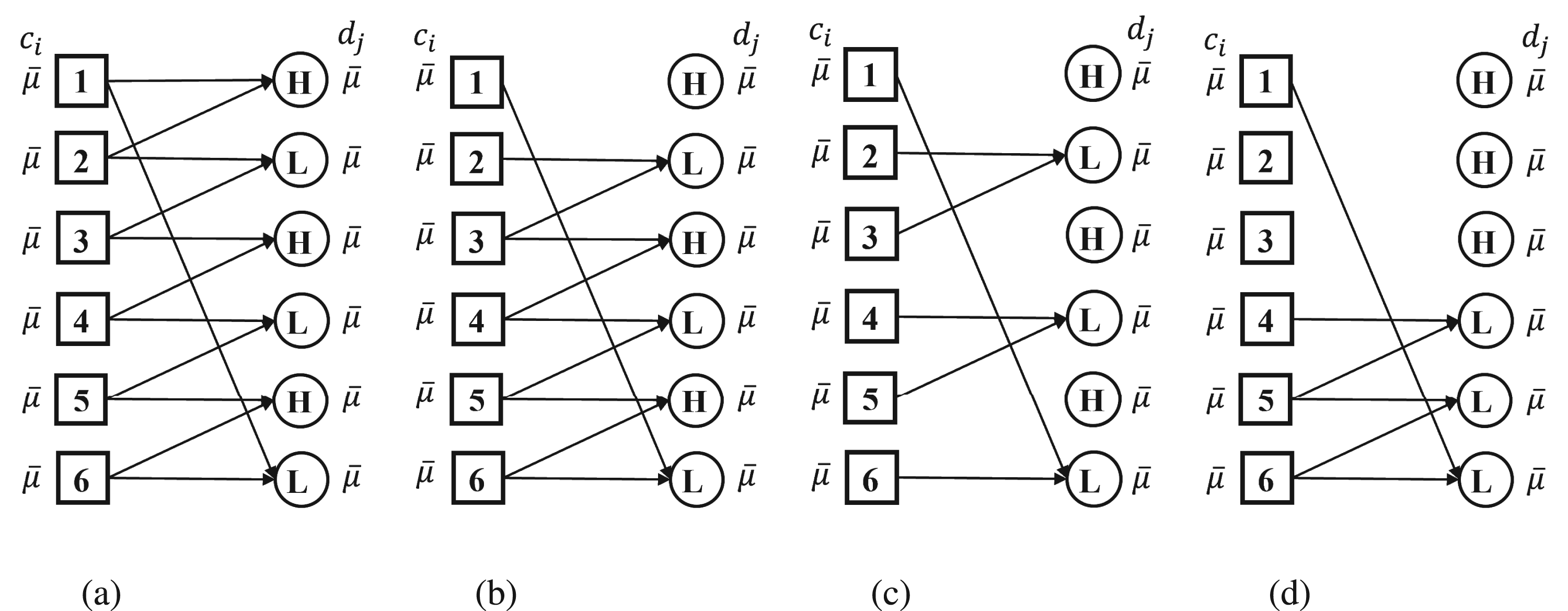
Beginning with the deterministic demand case, we examine how disruption risk affects flexibility design. Given the presence of differentiated marginal profits, we focus on the $A L$ , which was identified by Wang et al. (2022) as the optimal design under no disruption. For $T = 2$ , we introduce three long-chain structures: The design $A L$ , the sequential long chain ( $S L$ ), and the disjoint long chain ( $D L$ ). As shown in Figure 2(a) ( $n = 6$ ), $A L$ alternates between high- and low-margin products, with each plant producing one of each type. In contrast, $S L$ (Figure 2(b)) maintains a long-chain structure but allows consecutive products of the same margin to be produced by adjacent plants. The design $D L$ (Figure 2(c)) separates high- and low-margin products into two independent long chains. All three designs are 2-flexibility designs, meaning each product is linked to exactly two neighboring plants.

Figure 2.

Three classes of long chain. (a) $A L$ , (b) $S L$ and (c) $D L$ . $S L$ = sequential long chain; $D L$ = disjoint long chain; $A L$ = alternate long chain.

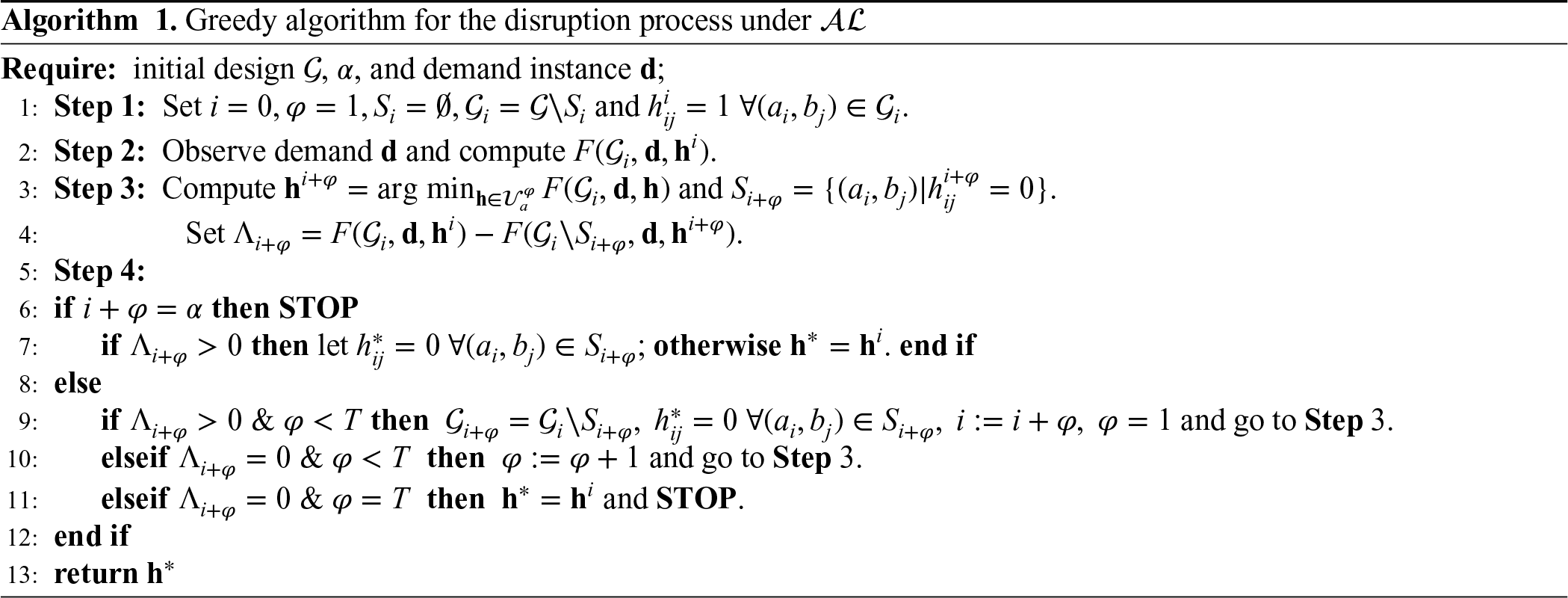
Before proceeding with the formal analysis, we delineate the scope of our study to balanced systems. While Problem (1) is applicable to arbitrary network configurations, we restrict our attention to the design $A L$ to avoid the trivial complications introduced by unbalanced systems. In this analysis, we set $γ = 0$ to isolate the impact of node-based disruptions and focus on their effect under the design $A L$ . We introduce a greedy algorithm to identify the worst-case disruption scenario in which the total profit loss resulting from disrupted arcs is maximized. The algorithm proceeds iteratively: In each step, it evaluates the marginal loss associated with the disruption of each individual arc and greedily selects the arc that leads to the greatest loss in the objective function. If disrupting any single arc in a given iteration does not reduce the objective value, the solution from the previous iteration is retained, and two arcs are jointly disrupted in the next step. This process continues until no further degradation in system performance is observed, or the predefined disruption budget is reached. The full procedure is outlined in Algorithm 1, which provides a pseudocode representation of the greedy disruption analysis.

In Algorithm 1, let $i$ denote the number of arcs that have already been disrupted in the current design $G_{i}$ . The parameter $φ$ denotes the number of arc-based disruptions in each iteration. In some iterations, when $φ = 1$ , the arc-based disruptions may not lead to any changes in system profit. Let $Λ_{i + φ}$ represent the change in the objective function value resulting from the disruption in the $(i + φ)$ th iteration. Based on these definitions, the following proposition establishes the optimality of the proposed greedy algorithm under the worst-case disruption analysis framework.

Proposition 1

Under the design $A L$ , for any given number of arc-based disruptions $α$ and any deterministic demand d, Algorithm 1 yields the optimal arc-based disruption solution.

Driven by the worst-case perspective, the disruption strategy aims solely to minimize the system’s total profit, which offers a clear rationale for the greedy algorithm. Under the $A L$ , Algorithm 1 provides an effective method for identifying worst-case arc-based disruptions once demand is realized. This enables managers to proactively assess system vulnerability and implement mitigation strategies accordingly. Although the greedy algorithm is introduced in the context of $A L$ —a structure with regularity and symmetry—the underlying worst-case disruption principle can be extended to more general long-chain configurations, which exhibit diverse structural patterns.

Example 1. When $T = 2$ , we compare the worst-case arc-based disruption scenarios under the $A L$ and the heterogeneous $S L$ , assuming all product demands are equal to $\bar{μ}$ and no node-based disruptions occur (i.e., $γ = 0$ ). As detailed in the Appendix, we find that in $A L$ , a plant node becomes effectively disrupted only when the number of disrupted arcs exceeds $n$ . In contrast, when products have identical marginal profits (i.e., $P_{H} = P_{L}$ ), the worst-case impact of disrupting two arcs is equivalent to that of losing an entire plant, since in both cases, the system suffers the loss of one unit of production capacity matching one unit of demand.

However, under the design $S L$ , the disruption of $n = 6$ arcs disables two plant nodes ( $a_{2}$ and $a_{3}$ , see Figure 3(d)). These plants are exclusively assigned to high-margin products and thus lack flexibility. Once the production of these products is disrupted, all output channels of the plants are blocked, resulting in node-based disruptions. Figures 3(c) and 3(d) illustrate the worst-case disruption scenarios under the $A L$ and $S L$ designs, respectively, when $α = 6$ , clearly demonstrating the superior resilience of the design $A L$ . This further underscores the research value of $A L$ in disruption-prone environments.

Figure 3.

Example 1. (a) $A L, α = 0$ , (b) $A L, α = 2$ , (c) $A L, α = 6$ and (d) $S L, α = 6$ . $S L$ = sequential long chain; $A L$ = alternate long chain.

In addition, we conducted an analysis of the frequency of arc failures that lead to node disruptions in Appendix EC.2.2. These results provide a quantitative characterization of the frequency with which worst-case disruptions correspond to node-based failures, reinforcing the structural relevance of node-based disruptions even under random arc failure scenarios. In the following subsection, we extend our analysis to incorporate demand uncertainty and evaluate the robustness of $A L$ using a robust optimization framework.

3.3. Analysis Under Uncertain Demand

Given the heterogeneous profit margins across product groups, we define an uncertainty set in which demand perturbations are symmetric within each product group. Following the formulation in Wang et al. (2022), we refer to this as the Partwise Independently Symmetric Perturbation (PISP) Uncertainty Set. Additionally, various alternative formulations for uncertainty sets are available in the literature (e.g., Bertsimas and Sim, 2004, Bertsimas and Brown, 2009).

Definition 1
(Partwise Independently Symmetric (PIS) Uncertainty Set). A set of uncertain demand $U_{d} \subseteq R_{+}^{n}$ is partwise independently symmetric if (i) $U_{d} = U_{1} \times \dots U_{T},$ and (ii) if $d_{V_{t}, - V_{t}} \in U_{d}$ , we have $d_{δ^{t} (V_{t}), - V_{t}} \in U_{d},$ where $δ^{t}$ is a permutation of $V_{t}$ .

In Definition 1, condition (i) states that demands for products with different margins are mutually independent, thereby establishing partwise independence. Condition (ii) stipulates that, for the products in the set $V_{t}$ , every permutation of the demand vector is equally likely to appear in the uncertainty set.
Definition 2
(Partwise Independently Symmetric Perturbation (PISP) Uncertainty Set). If $E := {d - μ}$ , where $d \in U_{d}$ , is PIS for a fixed $μ$ , then we call the set $U_{d} \subseteq R_{+}^{n}$ a PISP uncertainty set.

Then, for a given metric function $F (\cdot)$ associated with a flexibility design $G$ and uncertainty sets $U_{d}$ , $U_{a}$ , and $U_{p}$ , we define $R_{F} (G, U_{d}, U_{a}, U_{p})$ as the robust performance metric of $F (\cdot)$ . Specifically, $R_{F} (G, U_{d}, U_{a}, U_{p}) := min_{(d, h, g) \in U_{d} \times U_{a} \times U_{p}} F (G, d, h, g)$ represents the worst-case system performance under all realizations of the defined uncertainty sets. It is important to note that in the worst-case scenario, the cardinality constraints of the arc-based and node-based disruption sets are assumed to be tight, meaning exactly $α$ arcs and $γ$ plants are disrupted. To facilitate the comparison between different flexibility designs, we adopt the following definition from Mehmanchi et al. (2021).
Definition 3
Given uncertainty set $U$ , design $G_{1}$ is said to exhibit greater symmetric robustness than design $G_{2}$ if and only if $R_{F} (G_{1}, U) \geq R_{F} (G_{2}, U)$ .
3.3.1. Definition of MPGID

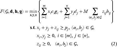
Note that Problem (1) is actually a weighted maximum flow problem. By dual theorem, the dual problem can be written as

\begin{aligned} F (G, d, h, g) = min_{x, y, z} & {\sum_{i = 1}^{m} x_{i} c_{i} g_{i} + \sum_{j = 1}^{n} y_{j} d_{j} + M \sum_{(a_{i}, b_{j}) \in G} z_{i j} h_{i j}} \\ s . t . & x_{i} + y_{j} + z_{i j} \geq p_{j}, (a_{i}, b_{j}) \in G, \\ x_{i}, y_{j} \geq 0, i \in [m], j \in [n], \\ z_{i j} \geq 0, (a_{i}, b_{j}) \in G, \end{aligned}

(2)

where dual variables

x = (x_{1}, \dots, x_{m})

y = (y_{1}, \dots, y_{n})

, and

z = {z_{i j}}

(\forall (a_{i}, b_{j}) \in G)

are assigned to the capacity constraints, demand constraints, and arc availability constraints of Problem (1), respectively. According to the complementary relaxation condition, we reformulate the dual problem.

Lemma 1

Problem (2) can be reformulated as the following linear program. Let $y^{*}$ denote a feasible solution satisfying the constraints of Problem (3). Then, for all $1 \leq j \leq n$ , it must hold that $y_{j}^{*} = p_{j} - p_{j^{'}}$ , where $0 \leq j^{'} \leq n$ , $p_{j^{'}} \leq p_{j}$ and $p_{0} ≜ 0$ .

\begin{aligned} F (G, d, h, g) = min_{x, y, z} & {\sum_{i = 1}^{m} x_{i} c_{i} g_{i} + \sum_{j = 1}^{n} y_{j} d_{j}} \\ s . t . & x_{i} + y_{j} + z_{i j} \geq p_{j}, (a_{i}, b_{j}) \in G, \\ z_{i j} h_{i j} = 0, (a_{i}, b_{j}) \in G, \\ x_{i}, y_{j} \geq 0, i \in [m], j \in [n], \\ z_{i j} \geq 0, (a_{i}, b_{j}) \in G . \end{aligned}

(3)

Since Problem (1) is a linear program, strong duality ensures that the optimal values of Problems (1) and (3) are equal. The dual problem in Equation (3) closely resembles the classical minimum cut problem, with an added complementary relaxation condition to account for arc-based disruptions. Moreover, Lemma 1 demonstrates that the optimal values of the dual variables are drawn from a discrete set. As the dual variables represent the shadow prices of the primal constraints, Lemma 1 implies a clear economic interpretation. Specifically, for an arc $(a_{i}, b_{j})$ , the dual variable $y_{j}^{*}$ indicates the marginal profit associated with increasing the demand for product $b_{j}$ by one unit. Its value depends on whether plant $i$ has sufficient residual capacity and whether it is disrupted. If $j^{'} = 0$ , then $y_{j} = p_{j}$ , which corresponds to a scenario with a local supply surplus—any additional demand for product $b_{j}$ can be satisfied using idle capacity. If $p_{j^{'}} = p_{j}$ , then $y_{j} = 0$ , indicating a local supply shortage—no additional capacity is available to satisfy increased demand. When $p_{j^{'}} < p_{j}$ , this reflects a supply-demand trade-off: The increased demand for product $b_{j}$ reallocates capacity originally used for product $b_{j^{'}}$ , generating an incremental profit of $p_{j} - p_{j^{'}}$ .

Furthermore, based on the result in Lemma 1, we formulate an MILP. Let $η_{t r} := P_{t} - P_{r}$ , where $0 \leq r \leq t$ and $1 \leq t \leq T$ . The term $η_{t r}$ represents the possible values of the dual variable $y_{j}$ for products $b_{j} \in V_{t}$ . We define an index set

K := {k_{t r} \in Z^{+} ∣ k_{t r} \leq | V_{t} |, r \in [t], t \in [T]},

where

k_{t r}

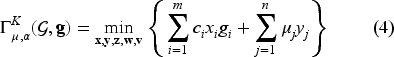
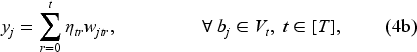
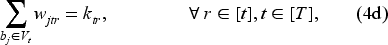
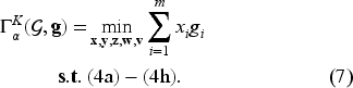
denotes the number of

y_{j}

values equal to

η_{t r}

for products in

V_{t}

. Given the average demand vector

μ

, the number of disrupted arcs

α

, the node status vector

g

, and the flexibility design

G

, we define the MPGID corresponding to the index set

K

Γ_{μ, α}^{K} (G, g)

, formulated as follows.

\begin{aligned} Γ_{μ, α}^{K} (G, g) = min_{x, y, z, w, v} {\sum_{i = 1}^{m} c_{i} x_{i} g_{i} + \sum_{j = 1}^{n} μ_{j} y_{j}} \end{aligned}

(4)

\begin{aligned} s . t . x_{i} + y_{j} + z_{i j} \geq p_{j}, \forall (a_{i}, b_{j}) \in G, \end{aligned}

(4a)

\begin{aligned} y_{j} = \sum_{r = 0}^{t} η_{t r} w_{j t r}, \forall b_{j} \in V_{t}, t \in [T], \end{aligned}

(4b)

\begin{aligned} z_{i j} = P_{T} v_{i j}, \forall (a_{i}, b_{j}) \in G, \end{aligned}

(4c)

\begin{aligned} \sum_{b_{j} \in V_{t}} w_{j t r} = k_{t r}, \forall r \in [t], t \in [T], \end{aligned}

(4d)

\begin{aligned} \sum_{(a_{i}, b_{j}) \in G} v_{i j} = α, \end{aligned}

(4e)

\begin{aligned} \sum_{r = 0}^{t} w_{j t r} = I {b_{j} \in V_{t}}, \forall t \in [T], \end{aligned}

(4f)

\begin{aligned} w_{j t r} \in {0, 1}, \forall b_{j} \in V_{t}, r \in [t], t \in [T], \end{aligned}

(4g)

\begin{aligned} v_{i j} \in {0, 1}, \forall (a_{i}, b_{j}) \in G . \end{aligned}

(4h)

In Problem (4), constraints (4b) and (4c) determine the feasible values of $y_{j}$ and $z_{i j}$ based on Lemma 1 and the parameter settings described above. To explicitly encode the values of $y_{j}$ and $z_{i j}$ , we introduce binary variables $w_{j t r}$ and $v_{i j}$ in constraints (4g) and (4h). Specifically, $w_{j t r} = 1$ indicates that $y_{j} = η_{t r}$ , and $v_{i j} = 1$ implies $z_{i j} = P_{T}$ ; otherwise, $y_{j} = 0$ and $z_{i j} = 0$ , respectively. Constraint (4d) enforces that exactly $k_{t r}$ variables $y_{j}$ take the value $η_{t r}$ for products $b_{j} \in V_{t}$ . Constraint (4e) specifies that exactly $α$ arcs are disrupted in the system, rather than allowing at most $α$ . Lastly, constraint (4f) ensures that the feasible values of $y_{j}$ remain consistent with the category-specific product group $V_{t}$ . In the Appendix EC.2.3 and EC.4, we provide additional details on the MPGID model and discuss its advantages over the distributionally robust model.

3.3.2. Robust Metrics

Using the MPGID defined in Problem (4), we derive an explicit representation of the robust metric $R_{F} (G, U_{d}, U_{a}, U_{p})$ . It is important to note that this robust metric remains a stochastic programing problem; the representation via MPGID serves as a structural decomposition rather than a closed-form solution. However, MPGID allows us to isolate and analyze the impact of flexibility design on the robust metric. Specifically, under identical parameter settings, different flexibility designs can be evaluated and compared through the partial order of their corresponding MPGID sets, thereby facilitating the identification of more robust design structures.

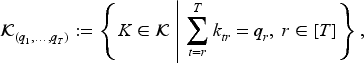
To this end, we first introduce some necessary notation. Let $U_{d}$ denote a PISP-type uncertainty set with a predefined mean demand vector $μ$ . For each product group $V_{t}$ , where $t \in [T]$ , define the corresponding mean demand subset as $μ_{V_{t}} = {μ_{j} ∣ b_{j} \in V_{t}}$ . Given a parameter set $K$ satisfying $0 \leq \sum_{r = 0}^{t - 1} k_{t r} \leq | V_{t} |$ where we omit the case of $r = t$ because $η_{t t} = 0$ does not affect the objective value in Problem (4), define the cumulative index $I_{t r} := \sum_{j = 0}^{r} k_{t j}$ for all $t$ and $r$ . Let $K$ denote the collection of all feasible parameter sets $K$ . Based on Proposition 2, we can identify an upper bound for the robust metric $R_{F} (G, U_{d}, U_{a}, U_{p})$ .

Proposition 2
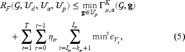
Given a flexibility design $G$ , an uncertain demand set $U_{d}$ , and disruption sets $U_{a}$ and $U_{p}$ , for any demand realization $d \in U_{d}$ and a parameter set $K = {k_{t r} \in Z^{+} ∣ 1 \leq t \leq T, 0 \leq r \leq t - 1}$ , we can derive an upper bound for the robust performance metric $R_{F} (G, U_{d}, U_{a}, U_{p})$ as
$\begin{aligned} R_{F} (G, U_{d}, U_{a}, U_{p}) \leq min_{g \in U_{p}} Γ_{μ, α}^{K} (G, g) \\ + \sum_{t = 1}^{T} \sum_{r = 0}^{t - 1} η_{t r} \sum_{i = I_{t r} - k_{t r} + 1}^{I_{t r}} {min}^{i} ϵ_{V_{t}}, \end{aligned}$
(5)
where, for every group $V_{t}$ , $ϵ_{V_{t}} := d_{V_{t}} - μ_{V_{t}}$ represent the demand residuals.

Then, an explicit representation of $R_{F} (G, U_{d}, U_{a}, U_{p})$ can be provided. Specifically, we show that there always exists a combination of a parameter set $K$ , a demand vector $d$ , and an arc-based disruption vector $h$ such that the upper bound given in Proposition 2 is tight.
Theorem 1
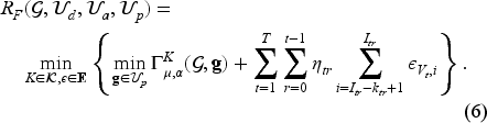
The robust metric of the production system under flexibility design $G$ , the PISP uncertainty set $U_{d}$ , the arc-based disruption set $U_{a}$ , and the node-based disruption set $U_{p}$ is given by
$\begin{aligned} R_{F} (G, U_{d}, U_{a}, U_{p}) = \\ min_{K \in K, ϵ \in E} {min_{g \in U_{p}} Γ_{μ, α}^{K} (G, g) + \sum_{t = 1}^{T} \sum_{r = 0}^{t - 1} η_{t r} \sum_{i = I_{t r} - k_{t r} + 1}^{I_{t r}} ϵ_{V_{t}, i}} . \end{aligned}$
(6)

Theorem 1 presents the expression for the maximum profit of the production system in the worst-case scenario, given a flexibility design and corresponding uncertainty sets. As shown in Problem (6), all components, except the MPGID, are independent of the flexibility design $G$ . Therefore, when evaluating the worst-case performance (WP) of the production system, our analysis focuses on the MPGID. Furthermore, Theorem 1 implies that, under a fixed uncertainty set, the symmetric robustness of different flexibility designs can be effectively compared by examining their corresponding MPGIDs.
Theorem 2
Suppose that $G_{1}$ and $G_{2}$ are two different flexibility designs. For a deterministic robust metric $R_{F} (\cdot)$ , if $Γ_{μ, α}^{K} (G_{1}, g) \geq Γ_{μ, α}^{K} (G_{2}, g)$ holds for all $K \in K$ , $g \in U_{p}$ , and $α$ , then we have $R_{F} (G_{1}, U_{d}, U_{a}, U_{p}) \geq R_{F} (G_{2}, U_{d}, U_{a}, U_{p}),$ for the uncertainty sets $U_{d}$ , $U_{a}$ , and $U_{p}$ . That is, design $G_{1}$ exhibits greater symmetric robustness than design $G_{2}$ .

Theorem 2 presents sufficient conditions for comparing different flexibility designs. Similar conditions have been proposed in the literature, such as in Mehmanchi et al. (2021), Simchi-Levi and Wei (2015), and Wang et al. (2022). In particular, Mehmanchi et al. (2021) established both necessary and sufficient conditions, albeit under the assumption of homogeneous products. In contrast, the setting considered in this paper is more general and accommodates heterogeneous product types.
4. Worst-Case Analysis of Alternate Long-Chain

In this section, we aim to investigate the performance of the design $A L$ under disruption risk. To facilitate the analysis, we begin by narrowing the scope of scenarios considered. Specifically, we focus on a balanced system in which the number of plants equals the number of products, both denoted by $n$ , where $n$ is an even integer no less than 4. The system involves two types of products with differentiated profit margins, that is, $T = 2$ . Let $P_{H}$ and $P_{L}$ represent the high and low profit margins, respectively. Define $V_{L} := V_{1}$ as the set of products with profit margin $P_{L}$ , and $V_{H} := V_{2}$ as the set of products with profit margin $P_{H}$ , with $| V_{H} | = | V_{L} | = n / 2$ . Following standard assumptions in long chain analyzes, we assume that each plant has an identical capacity normalized to 1. Additionally, the expected demand for all products is uniform, that is, $μ_{i} = μ_{j} = \bar{μ}$ for all $i, j$ .

Let $η_{10} = P_{L}$ , $η_{20} = P_{H}$ , and $η_{21} = P_{H} - P_{L}$ define the corresponding index set as $K = {k_{10}, k_{20}, k_{21}}$ . Due to the uniformity of expected demand, the term $\sum_{j = 1}^{n} μ_{j} y_{j}$ can be omitted for a given set $K$ without affecting the optimal solution of the model. For simplicity, we drop the subscript $μ$ and denote the MPGID as $Γ_{α}^{K} (G, g)$ , which is equivalent to the formulation in Problem (7)

\begin{aligned} Γ_{α}^{K} (G, g) = & min_{x, y, z, w, v} \sum_{i = 1}^{m} x_{i} g_{i} \\ s . t . & (4 a) - (4 h) . \end{aligned}

(7)

4.1. The Optimality of Alternate Long-Chain Under Disruption

In this subsection, the term “optimality” refers to achieving optimality in a long chain that consists of different combinations of plant-product links. This is opposed to being optimal in every 2-flexibility design, which is based on each product being exclusively linked to 2 plants. We will provide a more detailed explanation in the upcoming subsection.

Note that for arcs connected to product nodes with $y_{j} = P_{H}$ or $y_{j} = P_{L}$ , disruptions in such arcs $(a_{i}, b_{j})$ will not affect the total profit because $x_{i} = 0$ . The total number of such arcs is $2 k_{20} + 2 k_{10}$ . Therefore, we restrict our attention to cases where the total number of arc-based disruptions $α$ does not exceed $| G | - 2 k_{20} - 2 k_{10}$ . Furthermore, for any given $α \in [| G | - 2 k_{20} - 2 k_{10}]$ , we determine the MPGID value of the design $A L$ under $α$ arc-based disruptions using a sequential disruption approach. Lemma EC.1 provides an explicit characterization of $Γ_{α}^{K} (A L, g)$ for any given parameter set $K$ . It shows that when $k_{20} = n / 2$ , that is, in an over-supply scenario, the MPGID value of the design $A L$ suffers at most a profit loss of $P_{L}$ under arc-based disruptions. In this case, the demand for high-profit products is zero, and the system effectively degenerates into a single-product setting. However, as long as $k_{20} < n / 2$ and $k_{22} > 0$ , indicating that there exists unmet demand for high-profit products in the system, the worst-case loss due to arc-based disruptions leads to a profit loss of $P_{H}$ .

Meanwhile, Lemma EC.2 characterizes the MPGID values of $A L$ , $min_{g \in U_{p}^{γ}} Γ_{0}^{K} (A L, g)$ , when only plant nodes are disrupted. Based on Lemmas EC.1 and EC.2, we compare the MPGID values of $A L$ with those of the general long-chain design $L_{H L}$ . The following proposition summarizes the results of this comparison.

Proposition 3
For $T = 2$ and any parameter set $K \in K$ , we have the following results:
If $γ = 0$ , then $Γ_{α}^{K} (A L, e) \geq Γ_{α}^{K} (L_{H L}, e), 1 \leq α \leq 2 n - 2 k_{10} - 2 k_{20}$ .

If $α = 0$ , then $min_{g \in U_{p}^{γ}} Γ_{0}^{K} (A L, g) \geq min_{g \in U_{p}^{γ}} Γ_{0}^{K} (L_{H L}, g), 1 \leq γ \leq m$ .

Proposition 3 demonstrates that the MPGID of the design $A L$ consistently outperforms that of the $L_{H L}$ designs under any combination of demand parameters $K$ and disruption scenarios (arc or node). Notably, as indicated by the analysis in Theorem 1, the conclusion in Proposition 3 also holds in the case of deterministic demand (with a fixed $K$ ). Recall that the primary objective of this Section is to establish that the design $A L$ exhibits superior symmetric robustness compared to the $L_{H L}$ designs in production systems subject to disruptions. Based on Theorem 2, this result is formally presented in the following theorem.
Theorem 3
For any PISP uncertainty set $U_{d}$ :
When node-based disruption constraints are redundant, that is, $γ = 0$ and $g = 1$ , then for a symmetric arc-based disruption uncertainty set $U_{a}$ with parameter $α$ , it holds that $R_{F} (A L, U_{d}, U_{a}) \geq R_{F} (L_{H L}, U_{d}, U_{a})$ .

When arc-based disruption constraints are redundant, that is, $α = 0$ and $h = 1$ , then for a symmetric node-based disruption uncertainty set $U_{p}$ with parameter $γ$ , we have $R_{F} (A L, U_{d}, U_{p}) \geq R_{F} (L_{H L}, U_{d}, U_{p})$ .

Theorem 3 extends the findings of Wang et al. (2022) to scenarios involving supply disruptions and demonstrates that such disruptions do not compromise the optimality of the design $A L$ . In the absence of disruptions, the optimality of the design $A L$ arises from its key feature: Each plant simultaneously produces one high-profit and one low-profit product, thereby avoiding direct competition for shared resources among products with the same profit level. In contrast, the $L_{H L}$ designs allow some plants to produce both types of products concurrently, which introduces competition for limited capacity and may result in unfulfilled demand for high-margin products. When a supply disruption occurs—such as the failure of arc $(a_{i}, b_{j})$ —plant $a_{i}$ is no longer able to produce product $b_{j}$ . Under the $L_{H L}$ designs, the system may attempt to reallocate production through alternative plants to meet the demand for product $b_{j}$ , thereby intensifying competition among certain plants. However, since such a disruption removes a production link without intensifying resource contention at the plant level, the core advantage of the design $A L$ —namely, its separation of high- and low-margin product flows—remains intact. Therefore, even under identical disruption conditions, the design $A L$ continues to outperform $L_{H L}$ in terms of robustness and profit retention.

On the other hand, under node-based disruptions, the $L_{H L}$ designs assign certain plants exclusively to high-profit products. If these plants are disrupted, the corresponding high-profit demand is lost entirely, as other plants lack the flexibility to produce such products. This specialization also intensifies competition among the remaining plants when reallocating production. In contrast, the design $A L$ does not dedicate any plant solely to high-profit products. As long as not all plants are simultaneously disrupted, there will always be at least one operational plant capable of meeting high-profit demand. This structural flexibility allows the design $A L$ to outperform the $L_{H L}$ designs in terms of profit during node-based disruptions.

These results not only align with empirical observations—such as the supply chain strategies adopted by firms like Apple and AMD during periods of disruption (Stephen and Subrat, 2021)—but also provide theoretical support for employing design $A L$ to enhance supply chain flexibility and resilience. To validate Theorem 3, we conducted a series of numerical experiments under various parameter settings, with results summarized in Appendix EC.1. The findings confirm that the design $A L$ consistently outperforms the $S L$ design, even when arc-based and node-based disruptions occur simultaneously or under asymmetric stochastic demand, thereby demonstrating the robustness of our conclusion. On one hand, these results corroborate Theorem 3; on the other hand, they illustrate that the optimality of the design $A L$ persists even when the assumption of symmetric demand distributions is relaxed. Further analysis reveals the following insights: (i)
Under low-frequency arc-based disruptions (e.g., $α = 1$ ), both $A L$ and $S L$ designs experience increasing profit losses as demand variability rises. However, when arc-based disruptions are more frequent (e.g., $α = 3$ ), the profit losses stabilize.
(ii)
In the case of node-based disruptions, regardless of the disruption frequency, profit losses for both designs consistently increase with demand variability. This suggests that demand uncertainty exerts a more pronounced impact when production capacity is impaired.
(iii)
As the disruption frequency increases, the performance gap between $A L$ and $S L$ in terms of both average profit and performance relative to the full flexibility design becomes more significant with rising demand variability. However, this advantage is not monotonic in terms of WP.
(iv)
Given $α$ and $γ$ , as the profit margin of high-profit products increases, $A L$ exhibits strong robustness, particularly in terms of average performance (AP). In contrast, $S L$ demonstrates high sensitivity to this change, with substantial declines in both average and WP.
(v)
Additionally, we conducted numerical studies under asymmetric demand distributions that do not satisfy the PISP condition. Even in these scenarios, the design $A L$ consistently maintained its dominant performance.

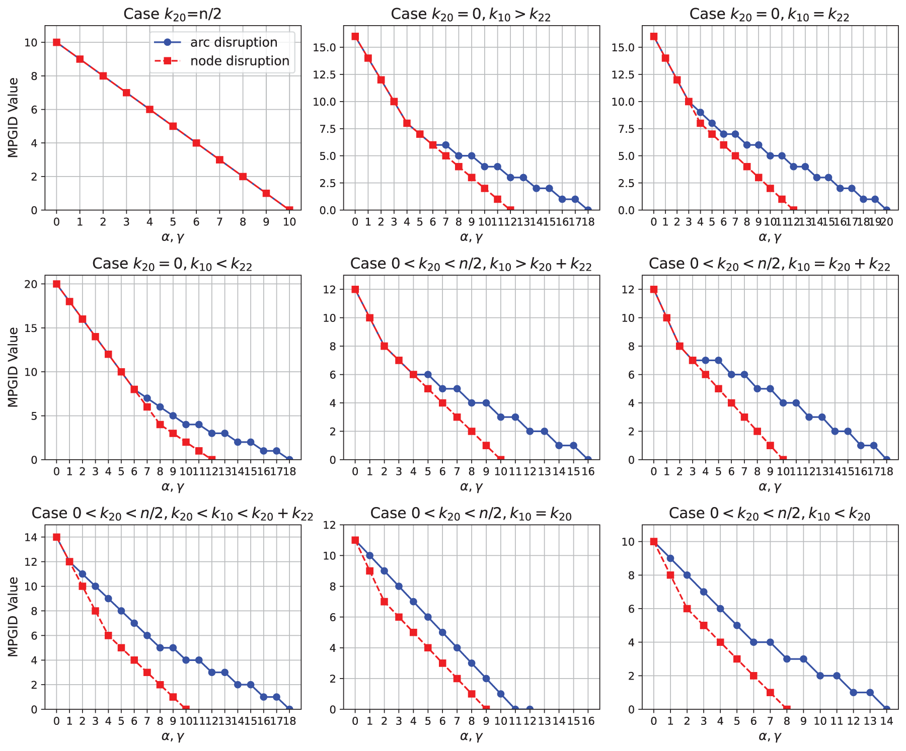
It is often assumed that node-based disruptions are more detrimental than arc-based disruptions, as the former lead to direct capacity losses, whereas the latter may be mitigated by system flexibility that allows continued production through alternative routes. However, by comparing Lemma EC.1 and Lemma EC.2—which provide explicit characterizations of the MPGID values for $A L$ under arc-based and node-based disruptions—we find that arc-based disruptions can, in many cases, be equally harmful. To illustrate this point, consider profit margins of $P_{H} = 2$ and $P_{L} = 1$ . We compute the MPGID values of the design $A L$ under various disruption scenarios. Figure 4 presents the resulting MPGID values across different demand conditions, corresponding to the nine distinct cases outlined in Lemma EC.1, when $α$ arcs and $γ$ plants are disrupted. This numerical comparison highlights the nuanced impacts of different disruption types and reveals that, under the design $A L$ , arc-based disruptions can lead to profit losses that are comparable to those caused by plant-level failures.

Figure 4.
The value of MPGID of $A L$ under different parameter settings. $A L$ = alternate long chain; MPGID = marginal profit group index under disruption.

The results reveal that the destructive impact of arc-based disruptions is more significant than initially anticipated. Specifically, when the disruption frequency is relatively low (e.g., $α, γ \leq 3$ ), arc-based disruptions often exert a comparable influence on system performance as node-based disruptions. However, as the number of disruptions increases, the marginal impact of arc failures gradually diminishes. This is because each plant node is typically connected to two arcs, and a disruption equivalent to a node failure requires both arcs to be simultaneously compromised. As a result, beyond a certain threshold, the losses caused by node-based disruptions begin to outweigh those from arc-based disruptions. This divergence in impact is influenced not only by the frequency of disruptions but also by the specific realizations of demand and the profit margin differential between products, captured by $P_{H} - P_{L}$ .
4.2. Fragility of Alternate Long-Chain

In this subsection, we examine the fragility—that is, the sensitivity—of long-chain designs under supply disruptions. Lim et al. (2011) first introduced the concept of fragility as a metric for evaluating the extent to which disruptions undermine the effectiveness of flexibility design, particularly in assessing the vulnerability of long chains. Mehmanchi et al. (2021) further demonstrated that in production systems with homogeneous profit margins, long chains tend to be more fragile than short chains under high disruption risk. In contrast, our findings reveal that when the number of disrupted arcs is sufficiently large, the design $A L$ exhibits larger fragility than designs $L_{H L}$ .

Assuming $γ = 0$ , we focus on analyzing the fragility induced by arc-based disruptions. By definition, $R_{F} (G, U_{d})$ measures the WP of flexibility design $G$ under demand uncertainty in the absence of disruptions. To evaluate the impact of arc-based disruptions, we define the fragility of design $G$ , denoted by $F r (G)$ , as the difference in robust performance with and without disruptions:

F r (G) := R_{F} (G, U_{d}) - R_{F} (G, U_{d}, U_{a}) .

This metric quantifies the vulnerability of a given flexibility design to supply-side disruptions, with higher values indicating greater sensitivity. According to Theorems 1 and 2, the fragility of a design can be analyzed through the MPGID. We begin by presenting the following lemma:

Lemma 2
There exists a threshold $α^{} \leq 2 n - 2 k_{10} - 2 k_{20}$ for any parameter set $K$ such that $Γ_{α}^{K} (A L, e) = Γ_{α}^{K} (L_{H L}, e), α \geq α^{}$ .

It is worth noting that while Lemma 2 establishes the existence of a threshold $α^{}$ , its specific value depends on the structure of demand uncertainty. When the demand for high-margin products in $V_{H}$ is relatively low and the demand for low-margin products in $V_{L}$ is relatively high, the corresponding $α^{}$ tends to be smaller. Conversely, when the demand for $V_{H}$ is high, $α^{}$ becomes significantly larger. In summary, when the disruption risk is sufficiently high—that is, when $α$ exceeds this threshold—the MPGID value under the design $A L$ becomes equal to that of the designs $L_{H L}$ for any given parameter set $K$ . Next, we present an intriguing result: When the number of disrupted arcs exceeds a certain threshold, design $A L$ becomes more fragile than general long chains under supply disruptions.
Proposition 4
Suppose $γ = 0$ , and the system experiences a substantial number of arc-based disruptions such that $α > α^{}$ . Then, the design $A L$ exhibits greater fragility than the general long-chain design, that is, $F r (A L) \geq F r (L_{H L})$ .

Differing from Mehmanchi et al. (2021), Proposition 4 is established within a multiproduct system, where both $A L$ and $L_{H L}$ represent long-chain designs. Nonetheless, our findings are consistent with the insights of Mehmanchi et al. (2021), which suggest that the optimal structure, in the absence of disruptions, tends to be more fragile under disruption risks. On the other hand, when disruptions are restricted to the plant level, the fragility measures of designs $A L$ and $L_{H L}$ coincide by the definition of the MPGID. This finding suggests that, within a multiproduct long-chain system, node-based disruptions exert only a modest influence on the design of process flexibility. Although fragility does not necessarily correlate with overall performance—a fragile design such as $A L$ may still achieve superior outcomes—this insight offers useful guidance for process flexibility planning. In practice, as noted by Sucky (2007), it is important to evaluate the maximum performance loss under real disruption scenarios. Risk-averse decision-makers may favor less fragile designs, as they ensure greater operational stability and more predictable responses to uncertainty.

Finally, we have discussed the limitations of the $A L$ design in the Appendix EC.2.4. Specifically, its optimality is valid only within the family of long-chain designs rather than across all 2-flexibility designs.
Remark 1
$A L$ is not the optimal design among all the 2-flexibility designs.
5. Generating Flexibility Designs and Experiments

Through the above discussion, we observe that there is no universally optimal design that effectively mitigates both supply disruption and demand uncertainty risks. Even the long-chain design, which generally performs well in enhancing process flexibility, proves inadequate under disruption scenarios. Therefore, this section proposes a heuristic algorithm aimed at generating flexibility designs capable of addressing both types of risks. We first develop an MPGID-based heuristic that accounts for both arc-based and node-based disruptions, and subsequently focus our analysis on arc-based disruption scenarios. The effectiveness and robustness of the proposed heuristic are validated through comprehensive numerical experiments.

5.1. MPGID-based Heuristic

In the literature on process flexibility, there are many algorithms for generating general sparse designs, such as Chen et al. (2018), Deng and Shen (2013), Simchi-Levi and Wei (2015), Mehmanchi et al. (2021) and Wang et al. (2022). Nevertheless, due to different research scenarios, most existing algorithms, generating flexible design, perform poorly in our setting. Therefore, we will propose a new heuristic algorithm based on MPGID to generate a flexibility design that effectively mitigates supply disruptions. We then compare our heuristic with other algorithms from the literature by evaluating the performances of these designs.

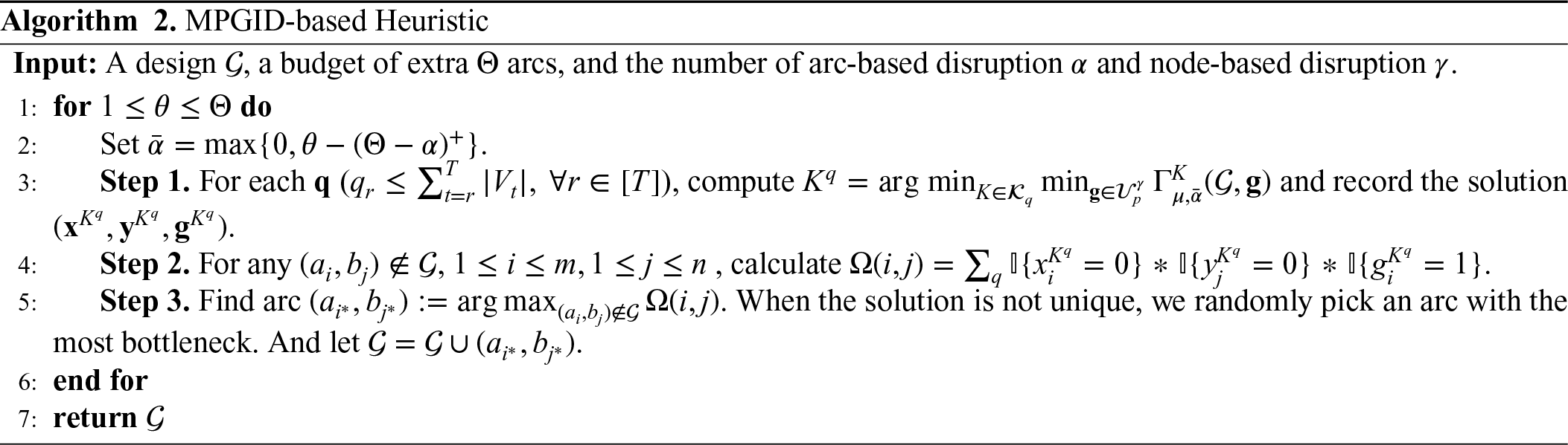
In the literature on process flexibility, numerous algorithms have been proposed for generating general sparse designs, such as those in Chen et al. (2018), Deng and Shen (2013), Mehmanchi et al. (2021), Simchi-Levi and Wei (2015), and Wang et al. (2022). However, due to differences in modeling assumptions and problem settings, most of these existing algorithms exhibit suboptimal performance in our context. To address this gap, we propose a novel heuristic algorithm based on the MPGID metric, which is developed specifically for scenarios that account for both supply disruptions and profit differentiation, and it remains applicable to unbalanced systems. We further compare the performance of our heuristic against benchmark algorithms from the literature by evaluating the resulting designs across multiple metrics. We declare that in each iteration, arcs are added with the goal of maximizing the marginal improvement of the MPGID value. Since the objective of Problem (4) is monotonically increasing with respect to $x_{i}$ and $y_{j}$ , Simchi-Levi and Wei (2015) defined a pair $(i, j)$ as a bottleneck if $x_{i} = 0$ and $y_{j} = 0$ . Such bottlenecks restrict the increase in MPGID and thus hinder robustness. To overcome this, in each iteration, we identify and add the arc $(a_{i}, b_{j})$ that corresponds to the most frequent bottlenecks across all demand scenarios. Moreover, the identification of bottlenecks should be limited to normal plants, that is, those with $g_{i} = 1$ . Accordingly, the arc to be added is selected as: $(a_{i^{*}}, b_{j^{*}}) = {\arg \max}_{1 \leq i \leq m, 1 \leq j \leq n} Ω (i, j)$ , where $Ω (i, j) := \sum_{K \in K} I {x_{i}^{K} = 0} \cdot I {y_{j}^{K} = 0} \cdot I {g_{i}^{K} = 1}$ .

On the other hand, according to the interpretation of the dual variables, if $x_{i}$ , $y_{j}$ , or $z_{i j}$ equals zero, it implies either capacity limitations or unmet demand (i.e., demand overflow) in the system. To reduce the computational burden of the algorithm, we restrict our attention to those scenarios $K$ that yield the worst-case MPGID values within a subset of $K$ denoted by $K_{(q_{1}, \dots, q_{T})}$ , which is indexed by an integer vector $(q_{1}, \dots, q_{T})$ . Specifically, we define

K_{(q_{1}, \dots, q_{T})} := {K \in K | \sum_{t = r}^{T} k_{t r} = q_{r}, r \in [T]},

where each

q_{r}

represents the number of products whose profit is at least

P_{r}

and whose corresponding dual variable

y_{j}

in Problem (4) equals

η_{t r}

. Given a plant status vector

g

and an integer vector

q := (q_{1}, \dots, q_{T})

with

0 \leq q_{r} \leq \sum_{t = r}^{T} | V_{t} |

, we evaluate the MPGID over all

K^{q} \in K_{q}

and determine the worst-case parameter set as

K^{q} := \arg min_{K \in K_{q}} min_{g \in U_{p}} Γ_{u, α}^{K} (G, g) .

Given an initial design $G$ , suppose that an additional $Θ$ arcs need to be added; this requires $Θ$ iterations. Since only the final $α$ arcs in the resulting design are subject to disruption, our analysis focuses on those last $α$ arcs introduced during the iterative process. Accordingly, we define the number of disrupted arcs in the $θ$ th iteration as $\bar{α} = max {0, θ - (Θ - α)^{+}}$ . In Step 1, we solve $min_{g \in U_{p}^{γ}} Γ_{μ, \bar{α}}^{K} (G, g)$ to obtain the dual solutions $x^{K^{q}}$ , $y^{K^{q}}$ and $g^{K^{q}}$ for all relevant parameter configurations $K^{q}$ . In Step 2, we count the number of bottlenecks each candidate arc—that is, those not yet included in the current design and plant $a_{i}$ has not been disrupted in the worst case—generates across different parameter settings $q$ . In Step 3, we add to the current design the arc with the highest bottleneck count. If multiple arcs tie for the highest count, one is selected randomly and uniformly. The complete procedure is summarized in Algorithm 2.

The MPGID-based heuristic algorithm adopts a robust optimization framework to generate general flexibility designs. To the best of our knowledge, this work is the first to address multiproduct flexibility design under the risk of supply disruptions. By leveraging the MPGID model, which inherently maximizes exposure to disruption risk, and building upon Theorem 2, the designs produced by the MPGID heuristic demonstrate strong robustness against both stochastic demand uncertainty and supply disruptions. This approach enables the construction of flexibility designs that are less vulnerable to disruptions compared to prior methods in the existing literature.

5.2. Numerical Experiments

Next, we demonstrate the superior performance of our proposed heuristic under disruption scenarios through a series of numerical simulations. Specifically, we compare the design $M$ generated by the MPGID-based heuristic with relevant designs and heuristics proposed in the existing literature. Furthermore, we analyze the marginal flexibility benefits of the MPGID heuristic and provide practical insights and recommendations for risk-averse decision-makers.

5.2.1. The Effectiveness of MPGID-based Heuristic

To evaluate the effectiveness and reliability of design $M$ , we compare its AP and WP ratios—both measured relative to the full flexibility benchmark—against designs generated by existing algorithms. The benchmark designs include: (i) Design $D$ , generated by the DMGI heuristic (Wang et al., 2022), which focuses on flexibility design in multiproduct production systems without considering supply disruptions; (ii) design $P$ , generated by the PCID heuristic (Mehmanchi et al., 2021), developed for settings with supply disruptions under homogeneous product assumptions; and (iii) design $S$ , obtained through the SAA method.

In the first set of experiments, we consider a balanced network comprising ten plants and ten products. Let $T = 2$ , where half of the products have a profit margin of $P_{H} = 2$ , and the other half have $P_{L} = 1$ . Given the maximum number of arc-based disruptions $α \in {3, 5}$ and node-based disruptions $γ \in {1, 2}$ , we apply the MPGID, DMGI, and PCID heuristic algorithms to generate flexibility designs containing 25 and 30 arcs, starting from a dedicated design as the initial structure. Additionally, 100 randomly generated demand samples are used to produce designs $S$ of the same size via the SAA method. The actual product demand $d_{i}$ are assumed to follow independent and identically distributed truncated normal distributions $N (μ_{i}, σ_{i})$ , truncated at zero.

For the designs generated by the above four methods, we conducted two tests: In test instances TEST1 and TEST2, we assign a average demand of 1 for all products, complemented by standard deviations of 0.4 and 0.8, respectively. Each plant possesses an identical capacity of 1 unit, $c_{i} = 1, \forall a_{i} \in A$ .

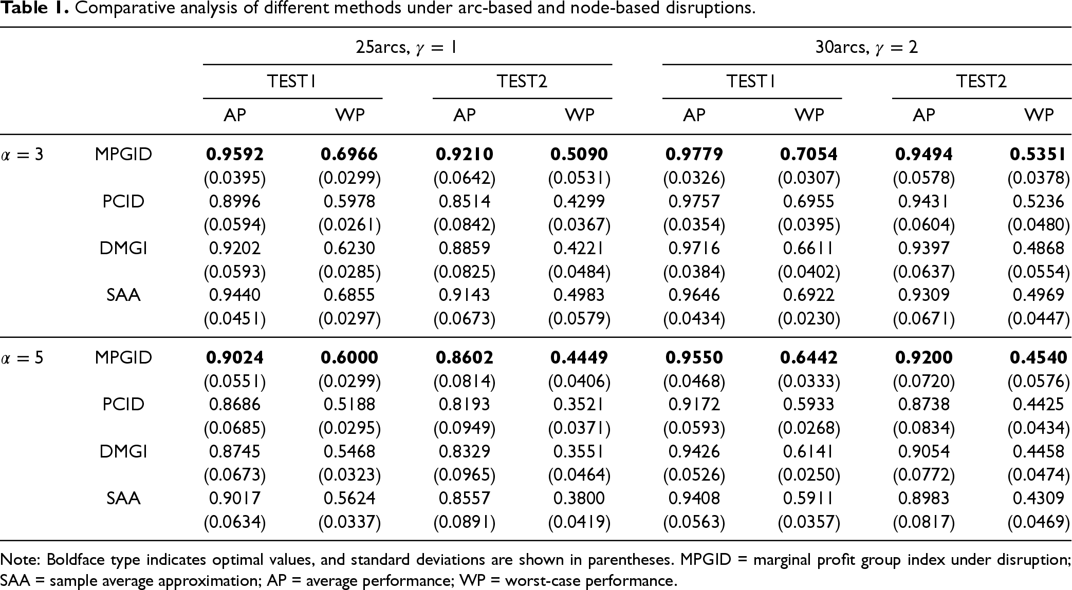
We generate 50 groups of samples, each containing 10,000 instances of demand and arc-based disruptions. In each instance, $α$ disrupted arcs and $γ$ disrupted nodes are randomly selected within the given design. For each group, we compute both the AP and WP of the various designs. It is worth noting that as the sample size increases, the likelihood of encountering extreme demand scenarios also rises, which may result in lower WP. In contrast, the AP tends to stabilize with larger sample sizes. Nonetheless, for a fixed sample size, the relative ordering (i.e., partial dominance) between different designs remains consistent. We also conducted experiments with larger-scale samples—such as 20,000 instances per group or 100 sample groups—and observed that the relative performance rankings of the designs remained unchanged. The results are presented in Table 1, and we find that:

(i)
The MPGID heuristic explicitly incorporates both disruption risk and demand uncertainty into the optimization process. As expected, the resulting design $M$ consistently achieves the best overall performance. Across various levels of demand variability (TEST1 vs. TEST2) and disruption frequency, the MPGID-based design outperforms others in both average and WP. This highlights a key insight: Optimizing for WP often yields strong AP as well, demonstrating the inherent robustness of the MPGID approach.
(ii)
A comparison between PCID and DMGI reveals that, under high supply risk or elevated demand volatility, the DMGI heuristic can outperform PCID. This is because DMGI incorporates differentiated profit margins, whereas PCID accounts for disruptions but assumes homogeneous margins. This finding highlights the critical importance of incorporating profit margin heterogeneity in process flexibility design. Notably, even in low-flexibility systems (e.g., with only 25 arcs), designs that do not explicitly consider disruptions can still exhibit substantial resilience—provided they effectively leverage profit-driven prioritization.
(iii)
Analysis of the SAA method shows that the resulting design $S$ often performs nearly as well as the MPGID-optimal design $M$ across many scenarios. This is intuitive, as the SAA samples include both stochastic demand realizations and randomly generated disruptions of arcs and plant nodes, enabling it to learn effective design structures from rich empirical data. However, the success of SAA depends heavily on the quality and representativeness of the samples. For rare events such as supply disruptions, obtaining sufficiently large and diverse sample sets (e.g., 100 scenarios) may be practically challenging in real-world applications.

Table 1.
Comparative analysis of different methods under arc-based and node-based disruptions.

25arcs, $γ = 1$ 30arcs, $γ = 2$

TEST1 TEST2 TEST1 TEST2

AP WP AP WP AP WP AP WP

$α = 3$ MPGID 0.9592 0.6966 0.9210 0.5090 0.9779 0.7054 0.9494 0.5351

(0.0395) (0.0299) (0.0642) (0.0531) (0.0326) (0.0307) (0.0578) (0.0378)

PCID 0.8996 0.5978 0.8514 0.4299 0.9757 0.6955 0.9431 0.5236

(0.0594) (0.0261) (0.0842) (0.0367) (0.0354) (0.0395) (0.0604) (0.0480)

DMGI 0.9202 0.6230 0.8859 0.4221 0.9716 0.6611 0.9397 0.4868

(0.0593) (0.0285) (0.0825) (0.0484) (0.0384) (0.0402) (0.0637) (0.0554)

SAA 0.9440 0.6855 0.9143 0.4983 0.9646 0.6922 0.9309 0.4969

(0.0451) (0.0297) (0.0673) (0.0579) (0.0434) (0.0230) (0.0671) (0.0447)

$α = 5$ MPGID 0.9024 0.6000 0.8602 0.4449 0.9550 0.6442 0.9200 0.4540

(0.0551) (0.0299) (0.0814) (0.0406) (0.0468) (0.0333) (0.0720) (0.0576)

PCID 0.8686 0.5188 0.8193 0.3521 0.9172 0.5933 0.8738 0.4425

(0.0685) (0.0295) (0.0949) (0.0371) (0.0593) (0.0268) (0.0834) (0.0434)

DMGI 0.8745 0.5468 0.8329 0.3551 0.9426 0.6141 0.9054 0.4458

(0.0673) (0.0323) (0.0965) (0.0464) (0.0526) (0.0250) (0.0772) (0.0474)

SAA 0.9017 0.5624 0.8557 0.3800 0.9408 0.5911 0.8983 0.4309

(0.0634) (0.0337) (0.0891) (0.0419) (0.0563) (0.0357) (0.0817) (0.0469)

Note: Boldface type indicates optimal values, and standard deviations are shown in parentheses. MPGID = marginal profit group index under disruption; SAA = sample average approximation; AP = average performance; WP = worst-case performance.

Finally, it is important to emphasize that while process flexibility design is intended to improve a system’s ability to match supply with demand under uncertainty, disruptions at the node level (i.e., plant failures) result in a direct and irreversible loss of supply capacity. As such, even designs that closely approximate full flexibility cannot fully mitigate the impact of node-based disruptions. In contrast, flexibility is more effective in addressing arc-based disruptions, where alternate pathways can be leveraged to reallocate capacity. Therefore, managing node-level risks often necessitates complementary strategies, such as maintaining safety stock or establishing emergency sourcing options, which lie beyond the scope of traditional flexibility design.

We assume $g_{i} = 1$ for all $a_{i} \in A$ , focusing exclusively on scenarios where only arc-based disruptions occur. In addition to TEST1 and TEST2, we further consider a generalized parameter setting (TEST3) and conduct an additional TEST4 to examine the validity of the model’s assumption—namely, the PISP uncertainty set for demand. The specific settings are as follows:

In TEST3, we analyze a case in which the demand distributions for high- and low-profit products are independent but differ in their statistical characteristics. Specifically, the high-profit product demands are $i . i . d .$ and follow a zero-truncated normal distribution with a mean of 1 and a standard deviation of 0.4, while the low-profit product demands are $i . i . d .$ and follow a zero-truncated normal distribution with a mean of 2 and a standard deviation of 0.8. The production capacity of each plant is uniformly set to 1.5 units.

In TEST4, we retain the baseline settings of TEST1 but introduce heterogeneity in the demand distributions within each product group to intentionally violate the PISP assumption. Specifically, for each profit category, the demands of three products follow a normal distribution (mean $μ_{i} = 1$ , standard deviation $σ_{i} = 0.4$ ), while the remaining two products follow a gamma distribution. Consequently, the demand structure does not satisfy the PISP uncertainty set within each group $V_{t}$ .

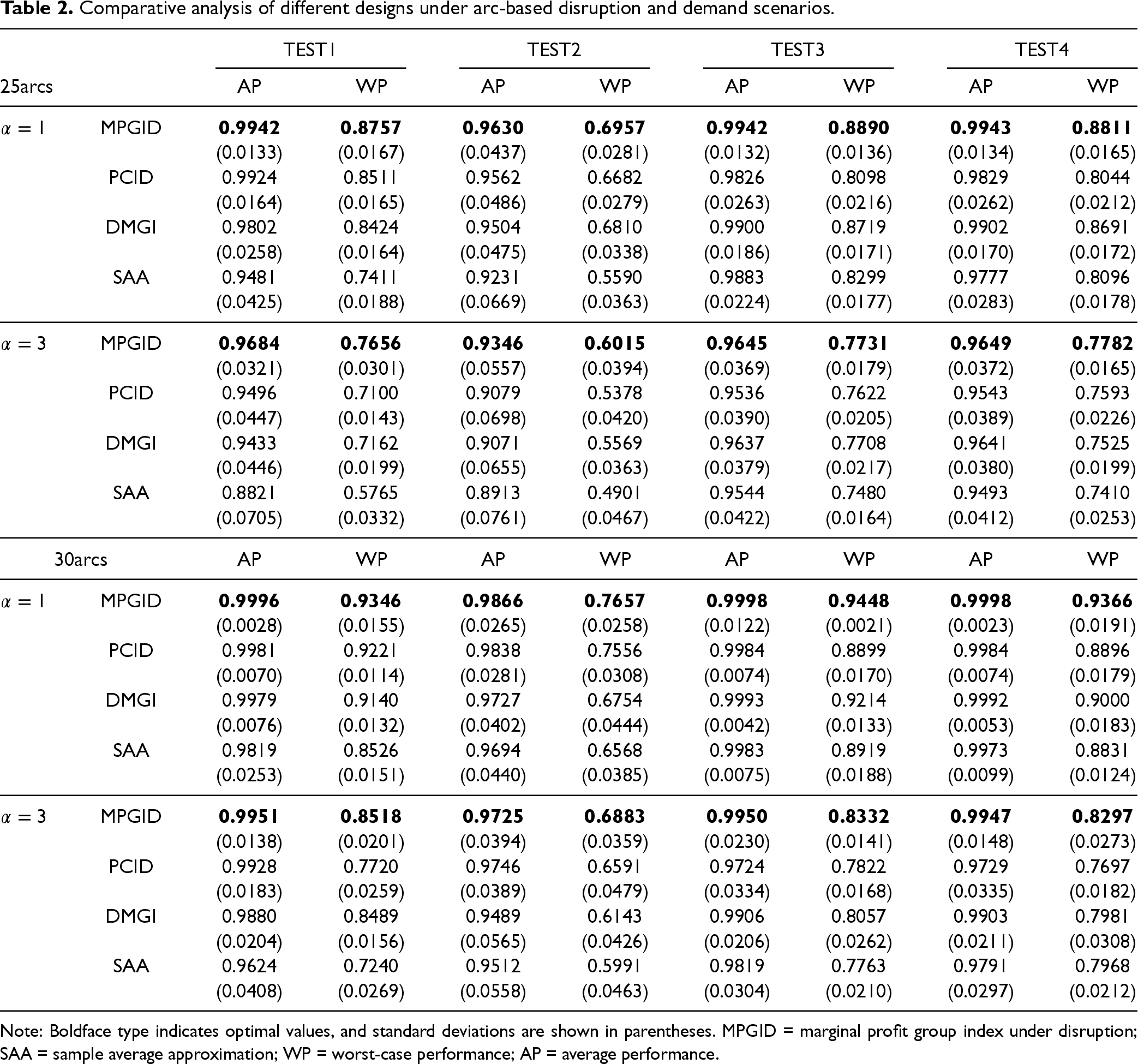
Table 2 presents the AP and WP ratios—calculated over 5,000 simulation samples—along with their corresponding standard deviations (in parentheses). These ratios evaluate the performance of the four designs with 25 and 30 arcs relative to full flexibility. Several key insights can be drawn from Table 2: (i)
To improve computational efficiency, we used a relatively modest sample size of 5,000 per test group. The standard deviations for all AP and WP estimates remain below 0.05 across all cases, except for TEST2 with a demand standard deviation of 0.8. This indicates that the performance metrics are statistically stable and reliable across simulations.
(ii)
In terms of AP ratios, design $M$ consistently outperforms the other designs, with its advantage becoming more pronounced as both demand variability and disruption risk increase. However, this advantage diminishes as system flexibility increases, reflecting convergence among the designs. In contrast, for WP ratios, design $M$ maintains a substantial advantage over other heuristics, although this dominance also narrows with increased flexibility. These findings align with expectations: Compared to the DMGI heuristic, the MPGID heuristic explicitly enhances robustness against disruption risks. Moreover, greater system flexibility naturally improves robustness, thereby reducing performance disparities between designs.
(iii)
Results from TEST4 confirm that our MPGID-based heuristic continues to outperform benchmark designs, even under asymmetric demand distributions. Comparing TEST3 and TEST4, we observe that asymmetric demand leads to a notable decline in WP values across all designs, while AP values remain largely unaffected. This suggests that asymmetry primarily complicates worst-case scenarios. Nonetheless, design $M$ continues to demonstrate strong resilience in such settings. Although the theoretical model assumes that stochastic demand satisfies the PISP condition, the strong empirical performance of the MPGID heuristic under non-PISP conditions highlights its robustness and potential for broader application in environments characterized by both stochastic demand and supply disruptions.

Table 2.
Comparative analysis of different designs under arc-based disruption and demand scenarios.

TEST1 TEST2 TEST3 TEST4

25arcs AP WP AP WP AP WP AP WP

$α = 1$ MPGID 0.9942 0.8757 0.9630 0.6957 0.9942 0.8890 0.9943 0.8811

(0.0133) (0.0167) (0.0437) (0.0281) (0.0132) (0.0136) (0.0134) (0.0165)

PCID 0.9924 0.8511 0.9562 0.6682 0.9826 0.8098 0.9829 0.8044

(0.0164) (0.0165) (0.0486) (0.0279) (0.0263) (0.0216) (0.0262) (0.0212)

DMGI 0.9802 0.8424 0.9504 0.6810 0.9900 0.8719 0.9902 0.8691

(0.0258) (0.0164) (0.0475) (0.0338) (0.0186) (0.0171) (0.0170) (0.0172)

SAA 0.9481 0.7411 0.9231 0.5590 0.9883 0.8299 0.9777 0.8096

(0.0425) (0.0188) (0.0669) (0.0363) (0.0224) (0.0177) (0.0283) (0.0178)

$α = 3$ MPGID 0.9684 0.7656 0.9346 0.6015 0.9645 0.7731 0.9649 0.7782

(0.0321) (0.0301) (0.0557) (0.0394) (0.0369) (0.0179) (0.0372) (0.0165)

PCID 0.9496 0.7100 0.9079 0.5378 0.9536 0.7622 0.9543 0.7593

(0.0447) (0.0143) (0.0698) (0.0420) (0.0390) (0.0205) (0.0389) (0.0226)

DMGI 0.9433 0.7162 0.9071 0.5569 0.9637 0.7708 0.9641 0.7525

(0.0446) (0.0199) (0.0655) (0.0363) (0.0379) (0.0217) (0.0380) (0.0199)

SAA 0.8821 0.5765 0.8913 0.4901 0.9544 0.7480 0.9493 0.7410

(0.0705) (0.0332) (0.0761) (0.0467) (0.0422) (0.0164) (0.0412) (0.0253)

30arcs AP WP AP WP AP WP AP WP

$α = 1$ MPGID 0.9996 0.9346 0.9866 0.7657 0.9998 0.9448 0.9998 0.9366

(0.0028) (0.0155) (0.0265) (0.0258) (0.0122) (0.0021) (0.0023) (0.0191)

PCID 0.9981 0.9221 0.9838 0.7556 0.9984 0.8899 0.9984 0.8896

(0.0070) (0.0114) (0.0281) (0.0308) (0.0074) (0.0170) (0.0074) (0.0179)

DMGI 0.9979 0.9140 0.9727 0.6754 0.9993 0.9214 0.9992 0.9000

(0.0076) (0.0132) (0.0402) (0.0444) (0.0042) (0.0133) (0.0053) (0.0183)

SAA 0.9819 0.8526 0.9694 0.6568 0.9983 0.8919 0.9973 0.8831

(0.0253) (0.0151) (0.0440) (0.0385) (0.0075) (0.0188) (0.0099) (0.0124)

$α = 3$ MPGID 0.9951 0.8518 0.9725 0.6883 0.9950 0.8332 0.9947 0.8297

(0.0138) (0.0201) (0.0394) (0.0359) (0.0230) (0.0141) (0.0148) (0.0273)

PCID 0.9928 0.7720 0.9746 0.6591 0.9724 0.7822 0.9729 0.7697

(0.0183) (0.0259) (0.0389) (0.0479) (0.0334) (0.0168) (0.0335) (0.0182)

DMGI 0.9880 0.8489 0.9489 0.6143 0.9906 0.8057 0.9903 0.7981

(0.0204) (0.0156) (0.0565) (0.0426) (0.0206) (0.0262) (0.0211) (0.0308)

SAA 0.9624 0.7240 0.9512 0.5991 0.9819 0.7763 0.9791 0.7968

(0.0408) (0.0269) (0.0558) (0.0463) (0.0304) (0.0210) (0.0297) (0.0212)

Note: Boldface type indicates optimal values, and standard deviations are shown in parentheses. MPGID = marginal profit group index under disruption; SAA = sample average approximation; WP = worst-case performance; AP = average performance.

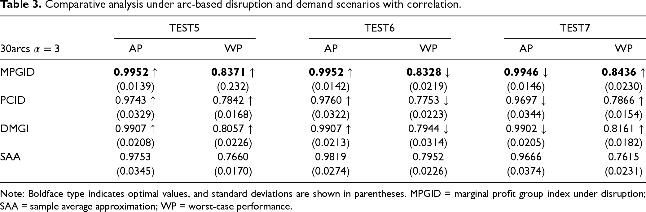
Given that the production system in this study involves multiple product types and our primary conclusions are derived under the assumption of demand independence, it is essential to examine whether the MPGID heuristic retains its advantage under demand distribution misspecification. Therefore, in the next set of numerical experiments, we introduce scenarios featuring varying degrees of correlation between the demands of the two product types. Specifically, in TEST5, TEST6, and TEST7, the parameter settings remain the same as those in TEST3, except that the correlation coefficients between the demands of high-profit and low-profit products are set to 0.4, 0.8, and $-$ 0.4, respectively. Although there exists inter-type correlation, the demands for products of the same type at different nodes remain independent. Consequently, the assumption that the demand uncertainty set satisfies the PISP still holds.

Table 3 shows that even when product demand correlations are not explicitly accounted for during the flexibility design process, the MPGID heuristic continues to exhibit strong robustness, significantly outperforming benchmark algorithms in both AP and WP profit ratios. This robustness holds across various correlation structures, as the MPGID consistently achieves the highest AP and WP values with relatively low standard deviations.

Table 3.
Comparative analysis under arc-based disruption and demand scenarios with correlation.

TEST5 TEST6 TEST7

30arcs $α = 3$ AP WP AP WP AP WP

MPGID 0.9952 $↑$ 0.8371 $↑$ 0.9952 $↑$ 0.8328 $↓$ 0.9946 $↓$ 0.8436 $↑$

(0.0139) (0.232) (0.0142) (0.0219) (0.0146) (0.0230)

PCID 0.9743 $↑$ 0.7842 $↑$ 0.9760 $↑$ 0.7753 $↓$ 0.9697 $↓$ 0.7866 $↑$

(0.0329) (0.0168) (0.0322) (0.0223) (0.0344) (0.0154)

DMGI 0.9907 $↑$ 0.8057 $↑$ 0.9907 $↑$ 0.7944 $↓$ 0.9902 $↓$ 0.8161 $↑$

(0.0208) (0.0226) (0.0213) (0.0314) (0.0205) (0.0182)

SAA 0.9753 0.7660 0.9819 0.7952 0.9666 0.7615

(0.0345) (0.0170) (0.0274) (0.0226) (0.0374) (0.0231)

Note: Boldface type indicates optimal values, and standard deviations are shown in parentheses. MPGID = marginal profit group index under disruption; SAA = sample average approximation; WP = worst-case performance.

Notably, previous work by Wang et al. (2022)—which did not consider arc-based disruptions—found that both positive and negative demand correlations could enhance flexibility performance by improving coordination or enabling diversification. However, our findings suggest that under arc-based disruption risk, this effect is no longer universally valid. Specifically, for AP, a positive demand correlation strengthens the pooling effect and enhances system resilience, whereas a negative correlation weakens this benefit. In terms of WP, moderate correlations (e.g., in TEST5 and TEST7) may offer some protection against extreme outcomes, but as the correlation becomes stronger, the probability of extreme joint demand realizations increases, which heightens vulnerability and degrades WP.

The critical difference stems from the presence of arc-based disruptions. Under such disruptions, correlated demands can exacerbate the propagation of local shocks, meaning that a single arc failure may result in disproportionately large cascading effects across the network. Consequently, instead of always delivering coordination advantages, demand correlation in the presence of disruptions may amplify systemic risk. These results highlight the need to jointly consider structural robustness and demand correlation when designing process flexibility under uncertainty. An effective robust design must not only ensure high average efficiency but also mitigate the amplification of worst-case scenarios driven by correlated demand and network-level disruptions.
6. Conclusion

		25arcs, $γ = 1$	30arcs, $γ = 2$
$α = 3$	MPGID	0.9592	0.6966	0.9210	0.5090	0.9779	0.7054	0.9494	0.5351
		(0.0395)	(0.0299)	(0.0642)	(0.0531)	(0.0326)	(0.0307)	(0.0578)	(0.0378)
	PCID	0.8996	0.5978	0.8514	0.4299	0.9757	0.6955	0.9431	0.5236
		(0.0594)	(0.0261)	(0.0842)	(0.0367)	(0.0354)	(0.0395)	(0.0604)	(0.0480)
	DMGI	0.9202	0.6230	0.8859	0.4221	0.9716	0.6611	0.9397	0.4868
		(0.0593)	(0.0285)	(0.0825)	(0.0484)	(0.0384)	(0.0402)	(0.0637)	(0.0554)
	SAA	0.9440	0.6855	0.9143	0.4983	0.9646	0.6922	0.9309	0.4969
		(0.0451)	(0.0297)	(0.0673)	(0.0579)	(0.0434)	(0.0230)	(0.0671)	(0.0447)
$α = 5$	MPGID	0.9024	0.6000	0.8602	0.4449	0.9550	0.6442	0.9200	0.4540
		(0.0551)	(0.0299)	(0.0814)	(0.0406)	(0.0468)	(0.0333)	(0.0720)	(0.0576)
	PCID	0.8686	0.5188	0.8193	0.3521	0.9172	0.5933	0.8738	0.4425
		(0.0685)	(0.0295)	(0.0949)	(0.0371)	(0.0593)	(0.0268)	(0.0834)	(0.0434)
	DMGI	0.8745	0.5468	0.8329	0.3551	0.9426	0.6141	0.9054	0.4458
		(0.0673)	(0.0323)	(0.0965)	(0.0464)	(0.0526)	(0.0250)	(0.0772)	(0.0474)
	SAA	0.9017	0.5624	0.8557	0.3800	0.9408	0.5911	0.8983	0.4309
		(0.0634)	(0.0337)	(0.0891)	(0.0419)	(0.0563)	(0.0357)	(0.0817)	(0.0469)

		TEST1	TEST2	TEST3	TEST4
$α = 1$	MPGID	0.9942	0.8757	0.9630	0.6957	0.9942	0.8890	0.9943	0.8811
		(0.0133)	(0.0167)	(0.0437)	(0.0281)	(0.0132)	(0.0136)	(0.0134)	(0.0165)
	PCID	0.9924	0.8511	0.9562	0.6682	0.9826	0.8098	0.9829	0.8044
		(0.0164)	(0.0165)	(0.0486)	(0.0279)	(0.0263)	(0.0216)	(0.0262)	(0.0212)
	DMGI	0.9802	0.8424	0.9504	0.6810	0.9900	0.8719	0.9902	0.8691
		(0.0258)	(0.0164)	(0.0475)	(0.0338)	(0.0186)	(0.0171)	(0.0170)	(0.0172)
	SAA	0.9481	0.7411	0.9231	0.5590	0.9883	0.8299	0.9777	0.8096
		(0.0425)	(0.0188)	(0.0669)	(0.0363)	(0.0224)	(0.0177)	(0.0283)	(0.0178)
$α = 3$	MPGID	0.9684	0.7656	0.9346	0.6015	0.9645	0.7731	0.9649	0.7782
		(0.0321)	(0.0301)	(0.0557)	(0.0394)	(0.0369)	(0.0179)	(0.0372)	(0.0165)
	PCID	0.9496	0.7100	0.9079	0.5378	0.9536	0.7622	0.9543	0.7593
		(0.0447)	(0.0143)	(0.0698)	(0.0420)	(0.0390)	(0.0205)	(0.0389)	(0.0226)
	DMGI	0.9433	0.7162	0.9071	0.5569	0.9637	0.7708	0.9641	0.7525
		(0.0446)	(0.0199)	(0.0655)	(0.0363)	(0.0379)	(0.0217)	(0.0380)	(0.0199)
	SAA	0.8821	0.5765	0.8913	0.4901	0.9544	0.7480	0.9493	0.7410
		(0.0705)	(0.0332)	(0.0761)	(0.0467)	(0.0422)	(0.0164)	(0.0412)	(0.0253)
30arcs	AP	WP	AP	WP	AP	WP	AP	WP
$α = 1$	MPGID	0.9996	0.9346	0.9866	0.7657	0.9998	0.9448	0.9998	0.9366
		(0.0028)	(0.0155)	(0.0265)	(0.0258)	(0.0122)	(0.0021)	(0.0023)	(0.0191)
	PCID	0.9981	0.9221	0.9838	0.7556	0.9984	0.8899	0.9984	0.8896
		(0.0070)	(0.0114)	(0.0281)	(0.0308)	(0.0074)	(0.0170)	(0.0074)	(0.0179)
	DMGI	0.9979	0.9140	0.9727	0.6754	0.9993	0.9214	0.9992	0.9000
		(0.0076)	(0.0132)	(0.0402)	(0.0444)	(0.0042)	(0.0133)	(0.0053)	(0.0183)
	SAA	0.9819	0.8526	0.9694	0.6568	0.9983	0.8919	0.9973	0.8831
		(0.0253)	(0.0151)	(0.0440)	(0.0385)	(0.0075)	(0.0188)	(0.0099)	(0.0124)
$α = 3$	MPGID	0.9951	0.8518	0.9725	0.6883	0.9950	0.8332	0.9947	0.8297
		(0.0138)	(0.0201)	(0.0394)	(0.0359)	(0.0230)	(0.0141)	(0.0148)	(0.0273)
	PCID	0.9928	0.7720	0.9746	0.6591	0.9724	0.7822	0.9729	0.7697
		(0.0183)	(0.0259)	(0.0389)	(0.0479)	(0.0334)	(0.0168)	(0.0335)	(0.0182)
	DMGI	0.9880	0.8489	0.9489	0.6143	0.9906	0.8057	0.9903	0.7981
		(0.0204)	(0.0156)	(0.0565)	(0.0426)	(0.0206)	(0.0262)	(0.0211)	(0.0308)
	SAA	0.9624	0.7240	0.9512	0.5991	0.9819	0.7763	0.9791	0.7968
		(0.0408)	(0.0269)	(0.0558)	(0.0463)	(0.0304)	(0.0210)	(0.0297)	(0.0212)

	TEST5	TEST6	TEST7
MPGID	0.9952 $↑$	0.8371 $↑$	0.9952 $↑$	0.8328 $↓$	0.9946 $↓$	0.8436 $↑$
	(0.0139)	(0.232)	(0.0142)	(0.0219)	(0.0146)	(0.0230)
PCID	0.9743 $↑$	0.7842 $↑$	0.9760 $↑$	0.7753 $↓$	0.9697 $↓$	0.7866 $↑$
	(0.0329)	(0.0168)	(0.0322)	(0.0223)	(0.0344)	(0.0154)
DMGI	0.9907 $↑$	0.8057 $↑$	0.9907 $↑$	0.7944 $↓$	0.9902 $↓$	0.8161 $↑$
	(0.0208)	(0.0226)	(0.0213)	(0.0314)	(0.0205)	(0.0182)
SAA	0.9753	0.7660	0.9819	0.7952	0.9666	0.7615
	(0.0345)	(0.0170)	(0.0274)	(0.0226)	(0.0374)	(0.0231)

This paper examines process flexibility design in production systems that are subject to supply disruption risks and stochastic product demands with differentiated profit margins. Supply disruptions are modeled as both arc-based (plant–product) and node-based (plant) failures. Under deterministic demand, we develop a greedy algorithm to identify the worst-case disruption scenario. We find that, in the worst case, the impact of sequential disruptions is equivalent to that of simultaneous disruptions. For stochastic demand, we reformulate the dual problem of maximizing profit into an MILP referred to as MPGID. Under a robust performance metric, we derive the maximum profit as a function of the designed MPGID values and a part-wise independently symmetric uncertainty set that characterizes demand variability. This framework significantly strengthens our ability to assess the impact of flexibility design under uncertainty.

Furthermore, MPGID enables effective comparison across different designs without requiring additional information on demand. Assuming two product types in the system, we characterize the MPGID outcomes under the design $A L$ and compare them with those from general long-chain designs. Our analysis reveals that, even under arc-based and node-based disruptions, the design $A L$ consistently outperforms other long-chain configurations, extending the conclusion in Wang et al. (2022). Numerical experiments show that, in certain cases, the severity of arc failures can be comparable to that of full plant shutdowns. Moreover, we demonstrate that the design $A L$ is less fragile—that is, less sensitive to disruption—than other long-chain designs when subjected to a sufficiently large number of arc failures.

Finally, we propose an MPGID-based heuristic algorithm. Across multiple test settings, this heuristic outperforms existing methods in scenarios with both uncertain supply and stochastic demand. Numerical results further indicate that jointly considering demand uncertainty and supply disruption risk significantly improves the effectiveness of process flexibility design. Among these factors, heterogeneity in marginal demand contributions exerts a more substantial impact on system profit than supply-side disruptions, underscoring the importance of prioritizing demand-side characteristics when aiming to optimize performance.

There are several directions in which this research can be extended or improved. First, more detailed modeling of marginal benefits could be considered. In our current model, marginal profits are associated only with product nodes. Another promising extension is to incorporate production costs on each arc (plant-product), as the cost of producing a product may vary across different plants. However, this would substantially increase the number of parameters in the model, posing significant challenges for MILP formulation and tractability. In addition, for large-scale systems, computing MPGID values for all $K \in K$ can be time-consuming. Developing efficient approximation or acceleration methods for this computation remains an important topic for future research.

Supplemental Material

sj-pdf-1-pao-10.1177_10591478251401432 - Supplemental material for Process Flexibility Analysis for Production Systems with Differentiated Margins Under Supply Risk

Supplemental material, sj-pdf-1-pao-10.1177_10591478251401432 for Process Flexibility Analysis for Production Systems with Differentiated Margins Under Supply Risk by Yuanguang Zhong, Xueliang Zheng, Wei Xie and Debiao Li in Production and Operations Management

Footnotes

Acknowledgments

The authors sincerely thank the Department Editor Professor Li Chen, the Senior Editor, and the two referees for their constructive and insightful comments on earlier versions of the paper. Xueliang Zheng, Wei Xie and Debiao Li are the corresponding authors.

Declaration of Conflicting Interests

The authors declared no potential conflicts of interest with respect to the research, authorship, and/or publication of this article.

Funding

The authors disclosed receipt of the following financial support for the research, authorship, and/or publication of this article: This work was supported by the National Natural Science Foundation of China (grant nos. 72325011, 72571066, 72171054 and 72321001) and Fujian Provincial Natural Science Foundation (grant no. 2023J06015).

ORCID iDs

Yuanguang Zhong

Xueliang Zheng

Wei Xie

Debiao Li

Supplemental Material

Supplemental material for this article is available online (doi: ).

How to cite this article

Zhong Y, Zheng X, Xie W and Li D (2026) Process Flexibility Analysis for Production Systems with Differentiated Margins Under Supply Risk. Production and Operations Management 35(6): 2241–2260.

References

Aksin

Karaesmen

(2007) Characterizing the performance of process flexibility structures. Operations Research Letters 35(4): 477–484.

Zeng

Zhang

, et al. (2014) Reliable p-median facility location problem: Two-stage robust models and algorithms. Transportation Research Part B: Methodological 64: 54–72.

Asghari

Al-e

Afshari

(2023) Disruption management for the electric vehicle routing problem in a geographically flexible network. Expert Systems with Applications 214: 119172.

Badakhshan

Ball

(2023) Applying digital twins for inventory and cash management in supply chains under physical and financial disruptions. International Journal of Production Research 61(15): 5094–5116.

Bertsimas

Brown

(2009) Constructing uncertainty sets for robust linear optimization. Operations Research 57(6): 1483–1495.

Bertsimas

Sim

(2004) The price of robustness. Operations Research 52(1): 35–53.

Chen

Chou

Sun

(2025) Process flexibility: A distribution-free approach to long chain resilience. Operations Research 0(0). https://doi.org/10.1287/opre.2023.0430 .

Chen

Zhang

, et al. (2018) Optimal design of process flexibility for general production systems. Social Science Electronic Publishing 67(2): 516–531.

Chen

Zhang

Zhou

(2015) Optimal sparse designs for process flexibility via probabilistic expanders. Operations Research 63(5): 1159–1176.

10.

Chou

Chua

Teo

, et al. (2010) Design for process flexibility: Efficiency of the long chain and sparse structure. Operations Research 58(1): 43–58.

11.

Chou

Chua

Teo

, et al. (2011) Process flexibility revisited: The graph expander and its applications. Operations Research 59(5): 1090–1105.

12.

Chou

Teo

Zheng

(2008) Process flexibility: Design, evaluation, and applications. Flexible Services and Manufacturing Journal 20(1-2): 59–94.

13.

Deng

Shen

(2013) Process flexibility design in unbalanced networks. Manufacturing & Service Operations Management 15(1): 24–32.

14.

Desir

Goyal

Wei

, et al. (2016) Sparse process flexibility designs: Is the long chain really optimal? Operations Research 64(2): 416–431.

15.

DeValve

Pekec

Wei

(2023) Approximate submodularity in network design problems. Operations Research 71(4): 1021–1039.

16.

Dong

Tomlin

(2012) Managing disruption risk: The interplay between operations and insurance. Management Science 58(10): 1898–1915.

17.

Feng

Wang

Shen

(2017) Process flexibility design in heterogeneous and unbalanced networks: A stochastic programming approach. IISE Transactions 49(8): 781–799.

18.

Harper

(2021) Suez blockage is holding up $9.6bn of goods a day. BBC News. https://www.bbc.com/news/business-56533250.

19.

Hendricks

Singhal

(2005) An empirical analysis of the effect of supply chain disruptions on long-run stock price performance and equity risk of the firm. Production and Operations Management 14(1): 35–52.

20.

Inajima

Okada

(2012) Japanese quake forces evacuation near nuclear reactor; oil refinery burns. https://www.bloomberg.com/news/articles/2011-03-11/cosmo-oil-refinery-set-on-fire-nuclear-power-reactors-shut-by-earthquake.

21.

Interos (2022) Build Operational Resilience into your Extended Supply Chain. https://www.interos.ai/solutions-operational-resilience/.

22.

Jin

Vergara

(2025) Greedy randomized adaptive search procedure for supply chain network resilience optimization considering risk diffusion. Journal of the Operational Research Society 76(5): 935–950.

23.

Jordan

Graves

(1995) Principles on the benefits of manufacturing process flexibility. Management Science 41(4): 577–594.

24.

Josephs

(2021) Pipeline outage forces American Airlines to add stops to some long-haul flights. CNBC. https://www.cnbc.com/2021/05/10/colonial-pipeline-shutdown-forces-airlines-to-consider-other-ways-to-get-fuel.html.

25.

Krishnamoorthy

Pramod

Chakravarthy

(2014) Queues with interruptions: A survey. Top 22: 290–320.

26.

Lim

Bassamboo

Chopra

, et al. (2011) Flexibility and fragility: Use of chaining strategies in the presence of disruption risks. (Preprint).

27.

Mak

Shen

(2009) Stochastic programming approach to process flexibility design. Flexible Services Manufacturing Journal 21(3-4): 75–91.

28.

Malcolm

(2011) After the disaster in Japan. https://www.automotivelogistics.media/after-the-disaster-in-japan/7408.article.

29.

Mehmanchi

Hoda

Oleg

(2021) Analysis of process flexibility designs under disruptions. IISE Transactions 53(2): 131–148.

30.

Piers

(2021) Stock take: Experts drill into the motor industry’s chip issues. Autocar. https://www.autocar.co.uk/car-news/industry-news-tech%2C-development-and-manufacturing/stock-take-experts-drill-motor-industrys.

31.

Ruiz-Torres

Mahmoodi

(2007) The optimal number of suppliers considering the costs of individual supplier failures. Omega 35(1): 104–115.

32.

Rujeerapaiboon

Zhong

Zhu

(2023) Resilience of long chain under disruption. European Journal of Operational Research 309(2): 597–615.

33.

Schmitt

Tomlin

(2012) Sourcing strategies to manage supply disruptions. In: Supply Chain Disruptions. London: Springer, pp. 51–72.

34.

Shen

Liang

Shen

(2021) Reliable hub location model for air transportation networks under random disruptions. Manufacturing & Service Operations Management 23(2): 388–406.

35.

Shi

Wei

Zhong

(2019) Process flexibility for multiperiod production systems. Operations Research 67(5): 1300–1320.

36.

Simchi-Levi

Schmidt

Wei

, et al. (2015) Identifying risks and mitigating disruptions in the automotive supply chain. Interfaces 45(5): 375–390.

37.

Simchi-Levi

Wei

(2012) Understanding the performance of the long chain and sparse designs in process flexibility. Operations Research 60(5): 1125–1141.

38.

Simchi-Levi

Wei

(2015) Worst-case analysis of process flexibility designs. Operations Research 63(1): 166–185.

39.

Snyder

Zümbül

Peng

, et al. (2016) Or/ms models for supply chain disruptions: A review. IISE Transactions 48(2): 89–109.

40.

Stephen

Subrat

(2021) Analysis-Apple, AMD navigate chip shortage with focus on profitable products. Euronews. https://www.euronews.com/next/2021/07/29/us-apple-semiconductors-analysis.

41.

Sucky

(2007) A model for dynamic strategic vendor selectio. Computers & Operations Research 34(12): 3638–3651.

42.

Tomlin

(2006) On the value of mitigation and contingency strategies for managing supply chain disruption risks. Management Science 52(5): 639–657.

43.

UNCTAD (2020) Review of maritime transport 2020. https://unctad.org/webflyer/review-maritime-transport-2020.

44.

Vidza

Budka

Chai

, et al. (2025) Supply network disruption: A framework for assessing vulnerability and implementing resilience strategies. Information Sciences 717: 122336.

45.

Wang

Zhang

(2021) A review of flexible processes and operations. Production and Operations Management 30(6): 1804–1824.

46.

Wang

Zhang

(2022) Robust optimization approach to process flexibility designs with contribution margin differentials. Manufacturing & Service Operations Management 24(1): 632–646.

47.

Wang

Zhang

(2015) Process flexibility: A distribution-free bound on the performance of k-chain. Operations Research 60(5): 1125–1141.

48.

Zhou

(2023) Commitment strategies and inventory decisions under supply disruption risk. Production and Operations Management 32(8): 2619–2637.

49.

Zhang

, et al. (2020) Online demand fulfillment under limited flexibility. Management Science 66(10): 4667–4685.

50.

Zhong

Zheng

Xie

(2025) Fulfillment flexibility strategy for dual-channel retail networks. IISE Transactions 57(1): 104–117.

Supplementary Material

Please find the following supplemental material available below.

For Open Access articles published under a Creative Commons License, all supplemental material carries the same license as the article it is associated with.

For non-Open Access articles published, all supplemental material carries a non-exclusive license, and permission requests for re-use of supplemental material or any part of supplemental material shall be sent directly to the copyright owner as specified in the copyright notice associated with the article.

0.00 MB

0.61 MB

		TEST1		TEST2		TEST3		TEST4
25arcs		AP	WP	AP	WP	AP	WP	AP	WP
$α = 1$	MPGID	0.9942	0.8757	0.9630	0.6957	0.9942	0.8890	0.9943	0.8811
		(0.0133)	(0.0167)	(0.0437)	(0.0281)	(0.0132)	(0.0136)	(0.0134)	(0.0165)
	PCID	0.9924	0.8511	0.9562	0.6682	0.9826	0.8098	0.9829	0.8044
		(0.0164)	(0.0165)	(0.0486)	(0.0279)	(0.0263)	(0.0216)	(0.0262)	(0.0212)
	DMGI	0.9802	0.8424	0.9504	0.6810	0.9900	0.8719	0.9902	0.8691
		(0.0258)	(0.0164)	(0.0475)	(0.0338)	(0.0186)	(0.0171)	(0.0170)	(0.0172)
	SAA	0.9481	0.7411	0.9231	0.5590	0.9883	0.8299	0.9777	0.8096
		(0.0425)	(0.0188)	(0.0669)	(0.0363)	(0.0224)	(0.0177)	(0.0283)	(0.0178)
$α = 3$	MPGID	0.9684	0.7656	0.9346	0.6015	0.9645	0.7731	0.9649	0.7782
		(0.0321)	(0.0301)	(0.0557)	(0.0394)	(0.0369)	(0.0179)	(0.0372)	(0.0165)
	PCID	0.9496	0.7100	0.9079	0.5378	0.9536	0.7622	0.9543	0.7593
		(0.0447)	(0.0143)	(0.0698)	(0.0420)	(0.0390)	(0.0205)	(0.0389)	(0.0226)
	DMGI	0.9433	0.7162	0.9071	0.5569	0.9637	0.7708	0.9641	0.7525
		(0.0446)	(0.0199)	(0.0655)	(0.0363)	(0.0379)	(0.0217)	(0.0380)	(0.0199)
	SAA	0.8821	0.5765	0.8913	0.4901	0.9544	0.7480	0.9493	0.7410
		(0.0705)	(0.0332)	(0.0761)	(0.0467)	(0.0422)	(0.0164)	(0.0412)	(0.0253)
30arcs		AP	WP	AP	WP	AP	WP	AP	WP
$α = 1$	MPGID	0.9996	0.9346	0.9866	0.7657	0.9998	0.9448	0.9998	0.9366
		(0.0028)	(0.0155)	(0.0265)	(0.0258)	(0.0122)	(0.0021)	(0.0023)	(0.0191)
	PCID	0.9981	0.9221	0.9838	0.7556	0.9984	0.8899	0.9984	0.8896
		(0.0070)	(0.0114)	(0.0281)	(0.0308)	(0.0074)	(0.0170)	(0.0074)	(0.0179)
	DMGI	0.9979	0.9140	0.9727	0.6754	0.9993	0.9214	0.9992	0.9000
		(0.0076)	(0.0132)	(0.0402)	(0.0444)	(0.0042)	(0.0133)	(0.0053)	(0.0183)
	SAA	0.9819	0.8526	0.9694	0.6568	0.9983	0.8919	0.9973	0.8831
		(0.0253)	(0.0151)	(0.0440)	(0.0385)	(0.0075)	(0.0188)	(0.0099)	(0.0124)
$α = 3$	MPGID	0.9951	0.8518	0.9725	0.6883	0.9950	0.8332	0.9947	0.8297
		(0.0138)	(0.0201)	(0.0394)	(0.0359)	(0.0230)	(0.0141)	(0.0148)	(0.0273)
	PCID	0.9928	0.7720	0.9746	0.6591	0.9724	0.7822	0.9729	0.7697
		(0.0183)	(0.0259)	(0.0389)	(0.0479)	(0.0334)	(0.0168)	(0.0335)	(0.0182)
	DMGI	0.9880	0.8489	0.9489	0.6143	0.9906	0.8057	0.9903	0.7981
		(0.0204)	(0.0156)	(0.0565)	(0.0426)	(0.0206)	(0.0262)	(0.0211)	(0.0308)
	SAA	0.9624	0.7240	0.9512	0.5991	0.9819	0.7763	0.9791	0.7968
		(0.0408)	(0.0269)	(0.0558)	(0.0463)	(0.0304)	(0.0210)	(0.0297)	(0.0212)

	TEST5		TEST6		TEST7
30arcs $α = 3$	AP	WP	AP	WP	AP	WP
MPGID	0.9952 $↑$	0.8371 $↑$	0.9952 $↑$	0.8328 $↓$	0.9946 $↓$	0.8436 $↑$
	(0.0139)	(0.232)	(0.0142)	(0.0219)	(0.0146)	(0.0230)
PCID	0.9743 $↑$	0.7842 $↑$	0.9760 $↑$	0.7753 $↓$	0.9697 $↓$	0.7866 $↑$
	(0.0329)	(0.0168)	(0.0322)	(0.0223)	(0.0344)	(0.0154)
DMGI	0.9907 $↑$	0.8057 $↑$	0.9907 $↑$	0.7944 $↓$	0.9902 $↓$	0.8161 $↑$
	(0.0208)	(0.0226)	(0.0213)	(0.0314)	(0.0205)	(0.0182)
SAA	0.9753	0.7660	0.9819	0.7952	0.9666	0.7615
	(0.0345)	(0.0170)	(0.0274)	(0.0226)	(0.0374)	(0.0231)