
Abstract
Emergency systems are designed to almost always have enough capacity to respond to emergencies. However, capacity shortage periods do occur and these systems need to recover quickly. In this study, we apply queueing models and study whether it is better for an emergency system to add or to expedite servers, in order to quickly recover from a capacity shortage period. We focus on emergency medical service (EMS) systems and use Erlang loss models to study Red Alerts (when all ambulances are busy) and Yellow Alerts (when the number of available ambulances falls below a threshold). We analyze two loss models: one with Markovian state‐dependent service rates and one with generally and independently distributed service times. We validate the two models against EMS data sets from two cities. Despite the fact that the distribution of ambulance service times is a mixture of lognormal distributions, which is far from being exponential, we find that the loss model with Markovian state‐dependent service rates provides a better representation of empirical Yellow and Red alert statistics. We build on the model with state‐dependent rates and use the theory of absorbing Markov chains to quantify the impact of adding or expediting ambulances, with respect to two performance measures: (i) the duration of alert periods, and (ii) the number of lost calls. This quantification helps EMS staff (dispatchers and supervisors) to make better decisions to avoid, and to recover from, alert periods. For example, staff should not wait until a Red Alert before adding ambulances, which is a common practice, because the expected number of lost calls rapidly increases as the number of available ambulances at the action epoch decreases.
Keywords
Introduction
Capacity shortage in a mission‐critical system like fire, police, and emergency medical service (EMS) can lead to a disaster if no contingency plans have been made. Although these systems are designed to almost always have enough capacity to respond to emergency calls in a timely fashion, contingency plans are needed to minimize the frequency with which the capacity is highly utilized, and to shorten the duration of capacity shortage periods if they do happen. Motivated by the EMS in Calgary and Edmonton, Alberta, Canada, that have been experiencing relatively frequent capacity (ambulance) shortage periods for several years, we focus on the specific context of EMS, and use queueing theory to provide insights on managing ambulance shortage periods.
Ambulance shortage periods are not limited to Alberta—they occur in EMS systems all over the world. For media and organizational reports from EMS in Australia, the US, and Canada (outside Alberta), see ABC News (2015), Zekman (2014), and Brown (2018), respectively.
EMS practitioners distinguish between high, medium, and low levels of resource utilization (Fitch et al. 1993). The terms used to describe these utilization levels vary among countries and regions. Calgary and Edmonton EMS refer to a High utilization as a “Red Alert,” which corresponds to a period when no ambulances are available to respond to new medical emergencies. They refer to a Medium utilization as a “Yellow Alert,” which corresponds to a period when the number of available ambulances is below a threshold θ (θ = 12 in Calgary; θ = 8 in Edmonton). In this study, we use Red Alert and Yellow Alert to refer to High and Medium utilization levels, respectively.
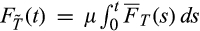
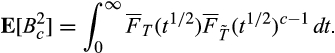
Yellow Alert periods are important from two perspectives: (i) the onset of a Yellow Alert is a signal to EMS staff to take actions to prevent the situation from deteriorating into a Red Alert, and (ii) a smaller number of available ambulances in the system increases the average distance between the call and the closest available ambulance, which results in longer response times. Practitioners view the threshold θ as the minimum number of ambulances needed to adequately cover the city’s geographical area. As Figure shows, average response time depends primarily on the number of available ambulances and is not highly sensitive to the number of scheduled ambulances (which varies with the call arrival rate). For these reasons, we keep θ fixed, independent of time, the number of scheduled ambulances, and the rate of call arrivals.
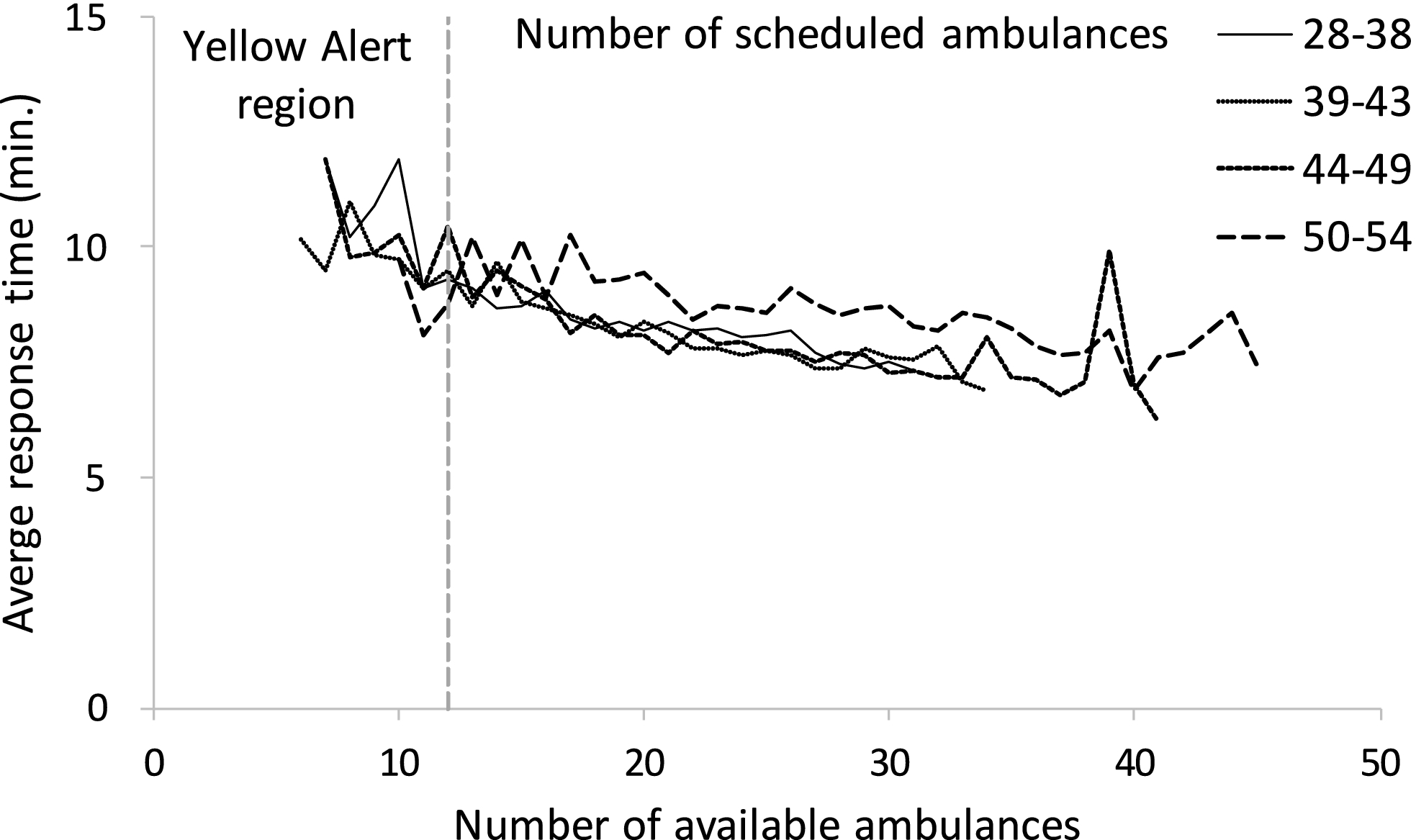
Average Response Time vs. the Number of Available Ambulances. Each Curve Corresponds to One Quartile for the Number of Scheduled Ambulances (Calgary 2009 Data). Only Data Points with a Sample Size of 10 or More are Shown
EMS staff manage Yellow and Red Alerts by taking three types of actions: expediting, adding, and repositioning ambulances. Expediting shortens “hospital time,” during which EMS crews wait to transfer patient care to emergency department (ED) staff. Expediting can be accomplished by: (i) expediting the admission of a patient occupying an ED bed into a hospital ward to free up the bed for an EMS patient, and (ii) consolidating the care of several waiting EMS patients under a single paramedic crew, allowing the other crews to leave the ED. Approach 1 requires collaboration and coordination between EMS and ED staff but Approach 2 can be carried out within the EMS. Adding ambulances could take the form of supervisors or managers asking for ambulances from neighboring municipalities, from another service (e.g., an interfacility‐transfer ambulance fleet), or asking new ambulance crews to come on duty. Adding ambulances usually requires collaboration and coordination between different EMS systems. Repositioning entails relocating available ambulances to improve the coverage of arriving calls. A simple and commonly used repositioning policy involves the use of a compliance table, which specifies target locations for all ambulances, as a function of the number of available ambulances.
Discussions with Calgary and Edmonton EMS staff indicate that they decide on actions based on a combination of judgment and rules that are implemented in a decision support system. A Red Alert is a simple rule that often triggers the adding of ambulances (Rumbolt 2017). A Yellow Alert is another trigger that indicates the staff should consider taking action but does not specify precisely which actions should be taken. The dynamics of EMS systems are sufficiently complex that it is difficult, even for highly experienced practitioners, to reliably predict the consequences of different actions using unaided human judgment. For example, the impact of adding ambulances depends on the remaining duration of the current alert period, which is difficult to predict, because alert period durations are highly variable, with squared coefficients of variation larger than one in most cases (Table 2). If the current alert period ends before the new ambulance(s) arrive, then cost will have been incurred and dispatchers, supervisors, and ambulance crews will have experienced added stress, all to no avail.
In this study, we do not attempt to estimate the cost of actions. Instead, we mathematically model alert periods and analyze the impacts of the expedite and add actions on these periods. We do not study repositioning because its impact on EMS operations has been investigated extensively by several researchers (Alanis et al. 2013, Maxwell et al. 2010, Schmid 2012).
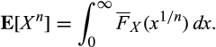
We model an EMS system as a loss (as opposed to delay) system, similar to other researchers (e.g., Maxwell et al. 2010, Restrepo et al. 2009), because the loss model is tractable, and calls that arrive during a Red Alert (which we refer to as “lost calls”) are typically served by other resources, such as the fire department or backup ambulance units, rather than waiting in a queue (Chong et al. 2015). We model Yellow and Red Alerts as special cases of “k‐partial busy periods”: time intervals during which k or more of the c scheduled ambulances are busy. Red Alerts are c‐partial busy periods and Yellow Alerts are (c − θ + 1)‐partial busy periods. Figure illustrates Yellow and Red Alerts when θ = 12 and c = 41. Every Red Alert is contained within a Yellow Alert, and a Yellow Alert can contain multiple Red Alerts.
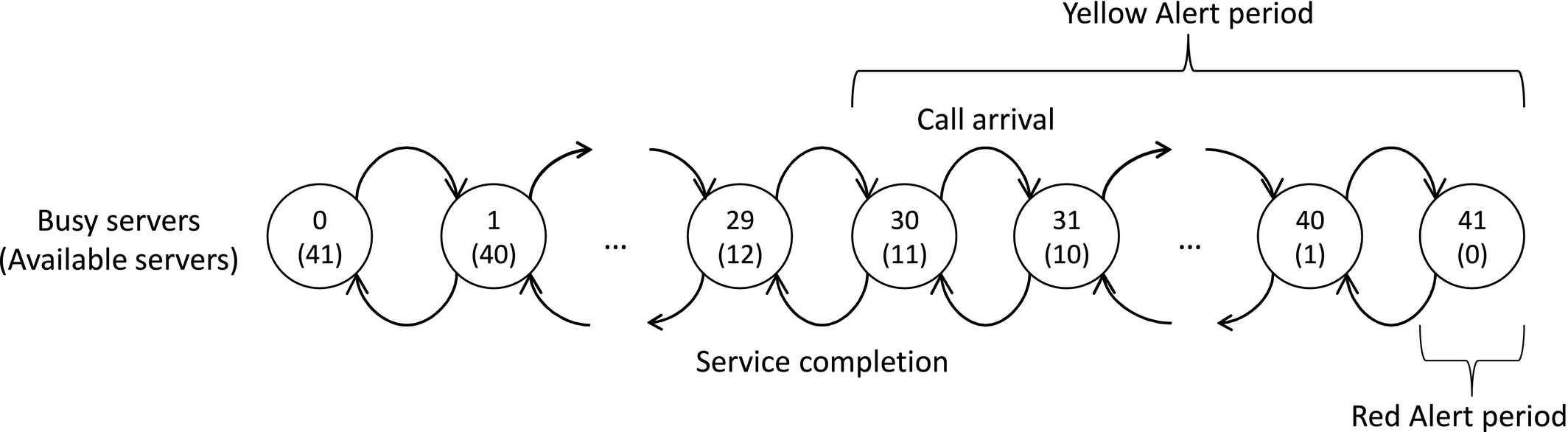
System States that Correspond to Yellow and Red Alerts. c = 41, θ = 12
We view an ambulance and its crew as a server, and we define the period from when a patient is assigned to a server, until the server becomes available again, as the service time. We thoroughly analyze the loss model with Markovian state‐dependent service rates, M/M(k)/c/c, and provide some results for the loss model with general service time, M/G/c/c. The former permits us to capture load‐based speedup or slowdown effects, and to indirectly capture some of the impacts of the spatial distribution of available ambulances, especially for systems in which compliance table policies are used to reposition ambulances. The latter permits us to model service times as a mixture of two distributions, for calls that are transported to hospital and those that are not.
We extend M/M(k)/c/c loss models to capture the impacts of add and expedite actions on alert periods through two performance measures: (i) the expected residual duration of a Yellow Alert and (ii) the expected number of lost calls. We provide insights on how the expedite and add actions compare with respect to these performance measures.
Our managerial contribution is that we show how to apply queueing models to quantify the impact of add and expedite actions on the expected remaining duration of Yellow Alert, and on the expected number of lost calls. For each performance measure, we use real EMS data and provide a threshold policy for comparing add and expedite actions as a function of the expected value of the time until actions are realized. We show that staff should not wait until a Red Alert occurs before taking action (which is a common practice), especially if the performance measure of interest is the expected number of lost calls, because that measure escalates rapidly as the number of available ambulances decreases. Another drawback of waiting too long before taking action is that the improvement in comparison with taking no action decreases, as the number of available ambulances at the action epoch decreases.
Our technical contribution is that we provide recursions to calculate the first and second moments of k‐partial busy periods for M/M(k)/c/c. We prove an insensitivity result for M/G/c/c that the first moments (but not higher moments) of k‐partial busy period durations depend on the service time distribution only through its mean. Using real EMS data, we show that although ambulance service rates depend strongly on the number of busy ambulances, and the service time distribution is a mixture of lognormal distributions, which is far from being exponential, the two loss systems perform similarly (M/M(k)/c/c is slightly better), with respect to predicting the mean of alert periods.
The remainder of the study is organized as follows. We review related literature in section 2; we define and analyze k‐partial busy period durations in section 3; we validate our models in section 4; we analyze the impacts of two actions, add and expedite, on two performance measures, expected remaining Yellow Alert duration and the expected number of lost calls, in section 5; we provide managerial insights on taking actions in section 6; and we conclude in section 7. Appendices A–H contain proofs, additional computational results, and a list of notation. All appendices may be found online in the Supporting Information section.
Literature Review
We survey four streams of related literature: (i) modeling of EMS systems, (ii) insensitivity results for loss systems, (iii) modeling of partial busy periods, and (iv) strategies to mitigate capacity or inventory shortages in various contexts.
EMS system models: Ingolfsson (2013) provides a recent general survey of research on planning and management for EMS systems. Modeling EMS systems as loss systems is common in this literature—either as a standard M/G/c/c system (Restrepo et al. 2009) or as a more general loss system (Alanis et al. 2013, Almehdawe et al. 2013, Chong et al. 2015, Li and Whitt 2014, Maxwell et al. 2010). We adopt the Erlang loss model for simplicity and to make progress on modeling the duration of partial busy periods and on modeling the impact of actions to mitigate capacity shortages. We assess the impact of some of the simplifications that are inherent in the Erlang loss model in section 4.
The impact of adding or expediting ambulances appears not to have been investigated before. Repositioning—another action that can be taken to mitigate capacity shortages—has been investigated by Alanis et al. (2013), Maxwell et al. (2010), Schmid (2012), and others. Our work complements theirs.
The Erlang loss model ignores two key aspects of EMS systems: Ambulances may not have the same service distribution, because of their geographic locations, and parameters (arrival rates and number of ambulances) vary with time or system state. Larson’s (1974, 1975) exact and approximate hypercube queueing models (HQM) address the geographic heterogeneity of ambulances. Many researchers have used variants of HQM to study EMS systems. Fewer researchers have explicitly incorporated time‐varying parameters in an analytical EMS system model; Ignall and Walker (1977) did this for an EMS system and Kolesar et al. (1975) for police patrol cars. Simulation models of EMS systems typically do incorporate time‐varying parameters (Henderson and Mason 2004, Mason 2013)
Evidence in Alanis et al. (2013) suggests that ambulance service rates depend on the number of busy ambulances. Erlang loss models with state‐dependent service rates have applications in traffic flow modeling (Jain and Smith 1997), and in designing evacuation networks (Weiss et al. 2012).
Insensitivity results for loss systems: Taylor (2011) defines an insensitive stochastic model as one whose “stationary distribution depends on one or more of its constituent lifetime distributions only through the mean,” and provides an extensive literature review. The best known insensitive stochastic models are M/G/c/c and M/G/∞.
Although the steady‐state probabilities of the M/G/c/c system are insensitive to the service time distribution beyond its mean, the same is not true for the transient occupancy probabilities. We show that the first moments of the k‐partial busy period durations, although they are measures of transient behavior, are insensitive to the service time distribution beyond its mean.
Partial busy periods: Busy periods are unambiguously defined and well studied for single‐server queues; they begin when a customer arrives to an empty system and last until the server becomes idle again for the first time. For analytical results, see, for example, Gross and Harris (1998) p. 102), For multi‐server queues, however, the terminology for busy periods varies. Omahen and Marathe (1978) use “busy period

Omahen and Marathe (1978) and Sharma (1990) studied k‐partial busy periods for the M/M/c and M/M/c/N (with queue capacity = N − c) systems, respectively. Bountourelis et al. (2013) observe that k‐partial busy periods have not been studied for loss systems, except as a special case of the M/M/c/N system. Our focus on loss systems allows us to obtain stronger results than those in Sharma (1990). Bountourelis et al. (2013) discuss applications of loss models in modeling hospital intensive care units (ICU) and highlight the importance of studying the length of periods during which ICUs are full, that is, c‐partial busy period durations. We thoroughly investigate k‐partial busy period durations, for k = 1,…,c, for Erlang loss systems with state‐dependent service rates and provide formulas to calculate their moments.
Shortage strategies: Protocols for managing ED capacity shortage have been formalized in an ED Surge Capacity Protocol in Alberta (Alberta Health Services 2010) and elsewhere (The College of Emergency Medicine 2014, Viccellio and Santora 2012) and medical researchers have investigated the impact of such protocols on ED crowding (Cha et al. 2009, Watase et al. 2012). Modelers have studied how to shift focus between triage and treatment when congestion in an ED exceeds a threshold (Zayas‐Caban et al. 2019). Alert periods are conceptually similar to low‐inventory periods for a retailer or a manufacturer, or periods where almost all beds in a hospital ward are occupied. Lawson and Porteus (2000), Duran et al. (2004), and Veeraraghavan and Scheller‐Wolf (2008) discuss the use of expediting during low‐inventory periods; that is, placing orders with a shortened lead time. Chan et al. (2014) investigate the use of speedup, modeled as a service rate increase, in an ICU in order to accommodate new patients that need to enter the ICU. Such short‐term actions are not without risk—for example, KC and Terwiesch (2012) show that speedup can increase the chance of ICU readmission and decrease an ICU’s peak capacity. We provide methods to compare the impacts of the adding and expediting actions on the expected residual Yellow Alert duration and the number of lost calls during the Yellow Alert.
Partial Busy Period Modeling
In this section, we model an EMS system where no actions are taken as a multi‐server loss system with Poisson arrivals and either Markovian state‐dependent service rates (M/M(k)/c/c), or a general service time (M/G/c/c).
We start with the M/M(k)/c/c system, which has a Poisson arrival process with rate λ, and has service rate


A k‐partial busy period, with duration


The M/M(k)/c/c Model
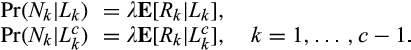
As illustrated in Figure , we decompose


A Schematic View of


We explicitly include conditioning in to stress that a k‐partial busy period always begins with an arrival. If the


The first two moments of


See appendix D.1.
The M/M/c/c system is a special case of M/M(k)/c/c, with

The Relationship Between the Loss Probability and Partial Busy Periods
The stationary loss probability for an M/G/c/c system is obtained from the Erlang B formula, the probability that all servers are busy (Gross and Harris 1998, p. 81). Here, we investigate the probability of experiencing Yellow and Red Alert periods during a k‐partial busy period. Let


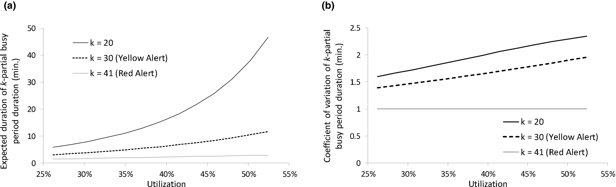
Impact of Utilization and k on Mean and Coefficient of Variation of Alert Durations
For an M/M(k)/c/c system, the probabilities


See appendix D.2.
Figure shows how


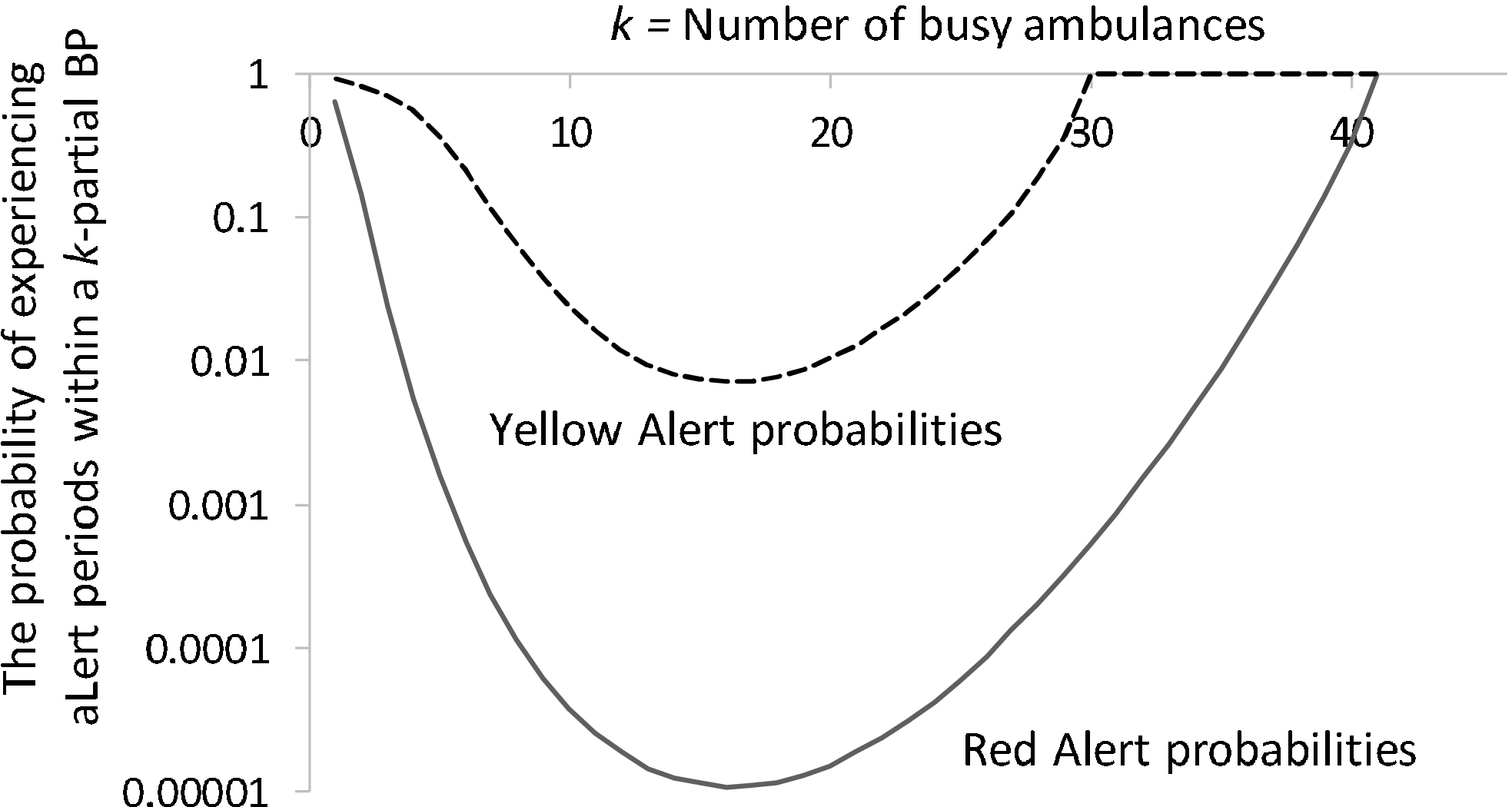
The Probability of Experiencing Yellow or Red Alert within a k‐Partial Busy Period as a Function of k
The M/G/c/c Model
Our calculations in section 3.1 relied heavily on the Markovian property. We develop our M/G/c/c formulas for


If the system has k busy ambulances, then we use


When there are k busy ambulances in the system, we calculate the probability of the next event by conditioning on the last event:
We use Equations and – to calculate the first moment of

The following hold for a stationary M/G/c/c system: The first moment of The second moment of The higher moments


See appendix D.3 for a precise stationary regime definition and a Theorem 3 proof.
Validation
We validate Equations , and – for the first and second moments of partial busy period durations for M/M(k)/c/c and M/G/c/c systems against data sets from Calgary and Edmonton, two cities with population of about 1 million in Alberta, Canada. The Calgary data set has 93,734 calls from 2009 and the Edmonton data set has 64,267 calls from 2008. Tables and provide fleet size, utilization, and descriptive statistics for EMS alert periods in these two cities. Utilization is computed as the average of the ratio of busy ambulances to scheduled ambulances. Yellow and Red Alerts were more frequent in Edmonton than Calgary, consistent with the higher average ambulance utilization in Edmonton.
Fleet Size and Utilization in Edmonton in 2008 and in Calgary in 2009
Descriptive Statistics for Alert Periods in Edmonton in 2008 and in Calgary in 2009
We show the validation results for Calgary in this section and discuss the Edmonton results in appendix F. We use the first 6 months as a training sample (used to compute all parameter estimates) and the second 6 months as a testing sample, for both data sets.
As inherent in standard Erlang loss models, in using - and (10), we implicitly assume that (i) the arrival rate and the number of scheduled ambulances are constants that do not vary with time or system state, (ii) the service rates do not vary with time, and (iii) all ambulances have the same service time distribution. In a real EMS system, however, arrival rates vary systematically by time of the day and day of the week (Channouf et al. 2007, Kim and Whitt 2014, Setzler et al. 2009); the number of scheduled ambulances changes by time of the day and day of the week; and the service time of an ambulance depends on its location and on the number and locations of other available ambulances. Figure illustrates how the arrival rate and the number of scheduled ambulances vary by time of the day in Calgary.
The Arrival Rate and the Number of Scheduled Ambulances vs. Time of the Day (Calgary 2009 Data)
We address these real‐world complications as follows: Instead of explicitly incorporating time‐varying parameters in our model (as Ignall and Walker (1977) did), we divide each week into 168 one‐hour segments and apply our model separately for each segment. We index the 1‐hour time segments using τ, with τ ranging from 1 for Sundays between midnight and 1 am to τ = 168 for Saturdays between 11 pm and midnight. We aggregate model outputs for the 1‐hour segments to obtain global model outputs. At the end of section 4.1, we outline reasons that suggest this method will be effective. We do not explicitly model ambulance locations, but the number of busy ambulances provides information about ambulance locations, because EMS dispatchers in Calgary and Edmonton use compliance tables to reposition ambulances (Alanis et al. 2013), that is, they try to achieve a pre‐specified configuration of locations for each number of busy ambulances. Service rates are likely to vary depending on the number of busy ambulances and the configuration of ambulance locations, and our M/M(k)/c/c model captures part of this dependence via the state‐dependent service rates.
Modeling of service times: We compare two modeling approaches for service times within each segment: general service times (G), and Markovian state‐dependent service times (M(k)).
For the general distribution approach, we fit a mixture of lognormal distributions with separate components for calls that are transported and not transported to hospital (appendix A), separately for each segment.
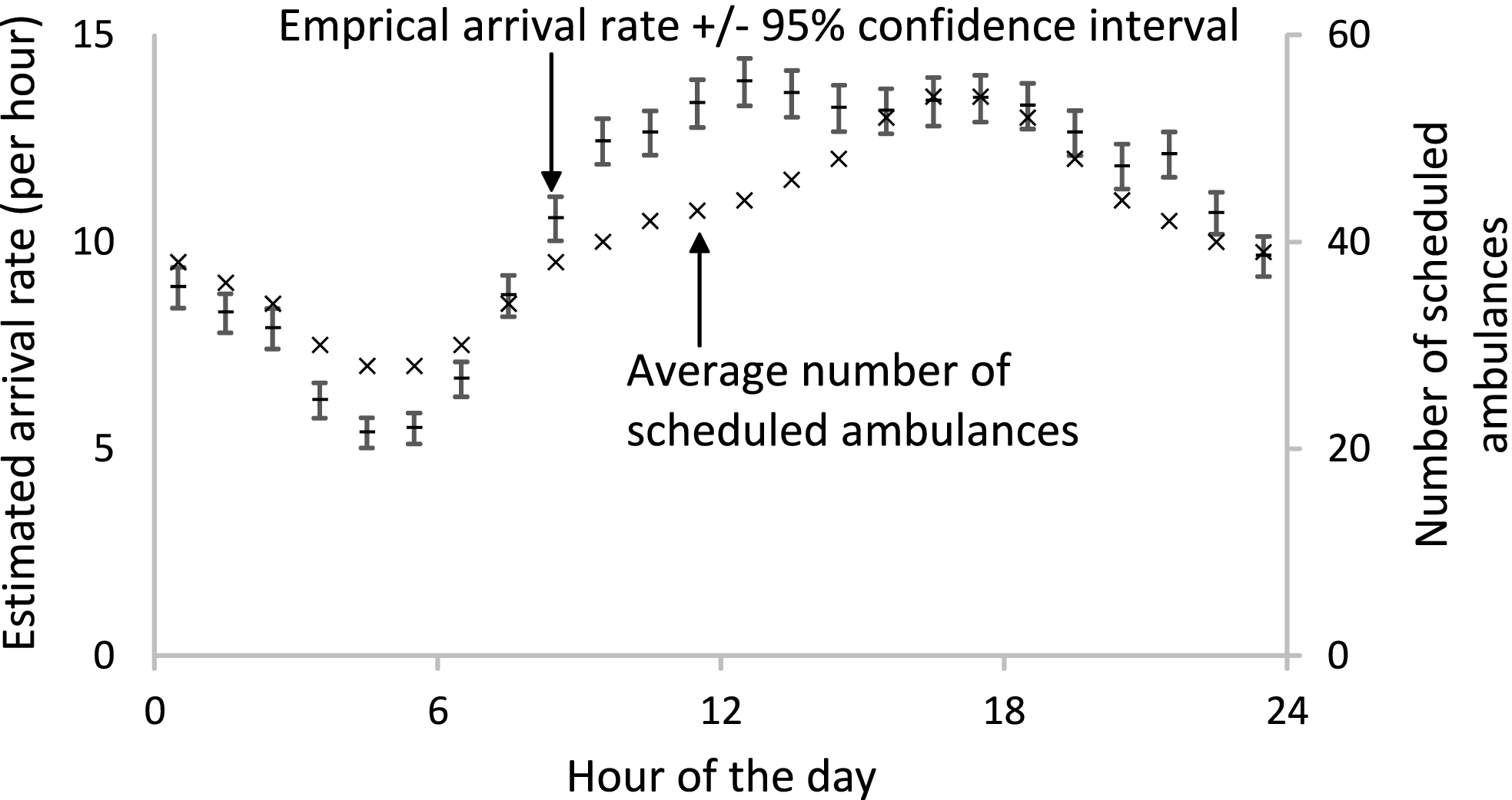
For the state‐dependent approach, we use a regression model to capture how mean service times vary with segment (Figure a) and with the number of busy ambulances (Figure b). The mean service time change by segment can be partially attributed to the change in traffic and transportation speed. By increasing the number of busy ambulances, the mean service time tends to increase; Alanis et al. (2013) hypothesize that this “slowdown” effect occurs because a large number of ambulance patient arrivals causes ED crowding, which increases the time that ambulances are tied up in EDs, which translates to longer average service times. Delasay et al. (2016) also argue that as the number of busy ambulances increases, the average travel distance from available ambulances to call locations increases, which increases the mean service time. Delasay et al. (2016) also discuss additional mechanisms through which the components of EMS service time vary with the number of busy ambulances.
Average Service Time vs. Number of Busy Ambulances and Hour of the Week (Calgary 2009 data)
To build our regression model, we compute the sample path for ν(t), the number of busy ambulances at t, by adding one at each call arrival epoch and subtracting one at each service completion epoch. We remove the data for 1 January and initialize ν(t) with the number of active calls at 0 am on 2 January, based on the assumption that none of these active calls arrived more than 24 hours before. KC (2013) used a similar approach to initialize a sample path for the number of busy physicians in an emergency department.
We estimate state‐dependent mean service time for Segment τ using a simple continuous piecewise linear regression model with a cutoff point at the Yellow Alert threshold, θ: 


The estimated intercept, slope, and Yellow Alert effect are 


Validation Using the Entire Sample
In this subsection, we perform out‐of‐sample validation using the entire data set. In section 4.2, we perform out‐of‐sample validation for each time segment separately. The validation process (both for the entire data set and separately for each time segment) consists of three steps: (i) estimate model primitives from the training sample, (ii) use the primitives to compute model outputs, and (iii) compare the model outputs to empirical outputs from the testing sample.
For validation, we take a weighted‐average approach, in which we first estimate model primitives separately for each time segment in the training sample, and use these segment‐specific primitives along with - and (10)–(12) to compute model outputs for each time segment, and then compute a weighted‐average of the segment‐specific model outputs to obtain global model outputs. We perform these steps for both ways of modeling services times (M(k) and G).
Model primitives: We use the superscript (τ) to indicate a notation is associated with Segment τ. For the weighted‐average approach, we estimate segment‐specific arrival rates 

Model outputs: We use - and (10)–(12) to compute segment‐specific model outputs 

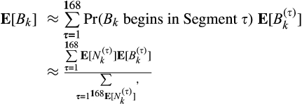

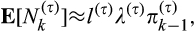


We use the same approach to approximate the second moment: 
We use the first and second moments of 

Empirical outputs: We use the ν(t) sample path of the testing data to compute samples of empirical k‐partial busy period durations 


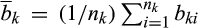
Figure illustrates our out‐of‐sample validation outcomes (Table 17 in appendix H shows the numerical values). Figure a compares the model and empirical means. It shows that model outputs for M(k) fit better than the ones for G, for small k, and they have very similar performance for large k, including those in the Yellow Alert region, which is the region of primary interest.

Empirical and Model Outputs for the Entire Sample (Calgary 2009 Data),
Figure b compares the model and empirical standard deviations. Here, we have G model outputs only for k = c. The M(k) model outputs overestimate the empirical outputs but the deviation is smaller in the Yellow Alert region, which is the region of primary interest.
To better understand the validation results, we note that the average arrival rate decreased by 0.84% from 10.74 in the training sample to 10.65 calls per hour in the testing sample, and the average service time decreased by 6.40% from 90.52 to 84.73 minutes, while the average number of scheduled ambulances remained at 41. Based on the decrease in workload, we would expect the periods when the system has a large number of busy ambulances to be shorter in the testing sample than in the training sample. Indeed, in Figure a, we see that the weighted average model outputs tend to be at the upper empirical confidence limits. In Figure b, we further see that the model outputs overestimate the empirical standard deviations, indicating that the k‐partial busy periods for high k in the testing sample were not only shorter, on average, but also less variable.
Perhaps the most important finding from this validation exercise is that even though the service time distribution is far from exponential, and service rates depend strongly on the number of busy ambulances, the two service time models (M(k) and G) result in model outputs that are very close (the M(k) model is slightly better). Our findings for the Edmonton data are similar. We already know from Theorem 3(a) that the first moments of partial busy periods are insensitive to the shape of the service time distribution beyond the mean, when service times are modeled as i.i.d. random variables. Our validation results supplement Theorem 3(a) with the numerical results that, for our data sets, the first moment is relatively insensitive to whether service times are modeled as state‐dependent (M(k)) or not (G). It appears that for the purpose of developing valid models of partial busy periods, changes over time, such as the reduction in workload we see between our training and testing samples, could be more important than how service times are modeled.
Transient vs. steady‐state analysis and the effectiveness of time segmentation: We use (16) and (17) to approximate 


Comparing the Steady‐State and Transient Approaches using the Entire Sample (Calgary 2009 Data)
We expect (consistent with results illustrated in Figure ) our time segmentation approach to be more reliable than what Green et al. (2001) results suggest, for the following three reasons: (i) EMS systems typically have lower utilizations than the systems studied by Green et al. (2001). For example, based on our data, the utilization is 43% in Calgary and 57% in Edmonton (Table ). (ii) Our model is a loss system, whereas Green et al. (2001) SIPP approach is for delay systems. Therefore, in our model, queues do not build up and queues do not propagate from one time segment to future time segments. (iii) Green et al. (2001) note that there is a lag between a peak in the arrival rate and a peak in congestion. Consequently, when the arrival rate is increasing, one expects steady‐state models for delay systems to overestimate the probability of delay and when the arrival rate is decreasing, one expects steady‐state models to underestimate the probability of delay. We aggregate model outputs for the 1‐hour segments to obtain global model outputs, which implies that the overestimation and underestimation errors cancel out to some extent.
Validation by Segment
Our findings so far are that global model outputs computed using a weighted‐average of segment‐specific model outputs fit well with global empirical outputs. We would also like to know, however, how well the model outputs for a particular segment match empirical outputs for that segment, as that comparison provides an indication of the utility of our models for predicting alert period durations in real time. In this subsection, we perform this comparison, as a further validation step.
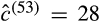
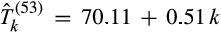
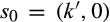
We perform out‐of‐sample validation for our model against each segment by using the same three validation steps listed in section 4.1, for the entire sample. To demonstrate our validation steps, however, we focus on the busiest segment in the training data, Wednesday 1–2 pm, τ = 86 (with 344 calls and 27.91 busy ambulances on average), and the least busy segment in the training data, Tuesday 4–5 am, τ = 53 (with 113 calls and 6.52 busy ambulances on average). We focus on these two segments to show that our model provides good results both for segments with a high and a low number of busy ambulances.
Model primitives: For the busiest segment, we estimate the arrival rate to be 

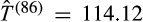
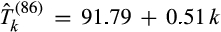
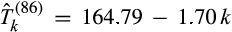
For the least busy segment, our estimates are 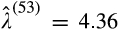

Model outputs: We compute the segment‐specific model outputs as described in section 4.1.
Empirical outputs: We would like the empirical outputs for Segment τ to be representative of conditions during that time segment. Therefore, we do not use empirical outputs based on the entire sample. A possible approach would be to use only k‐partial busy periods that are fully contained within Segment τ, but this approach would severely bias the analysis, because partial busy periods that span more than one hour tend to be longer, on average, than those contained within an hour. Instead, we construct separate sample paths for each segment, by concatenating the 26 one‐hour periods of observations that we have for each segment.
Appendix B describes the concatenation procedure. We follow the same process as we did for the entire sample to construct the sample path and calculate the empirical outputs for each segment. The concatenated sample paths are not used in the estimation of model primitives, the calculation of model outputs, or in the aggregate validation in section 4.1—they are only used to calculate segment‐specific empirical outputs.
Figures and compare model and empirical outputs for the busiest and least busy segments. The model outputs are generally within the 95% confidence intervals for the empirical outputs, especially for high values of k, which correspond to Yellow and Red Alerts. The model outputs for the two service time models are almost indistinguishable for high k values.
Empirical and Model Outputs for the First Moment (Calgary 2009 Data)
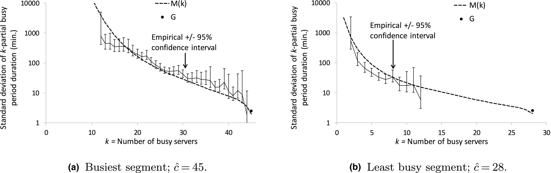
Empirical and Model Outputs for the Standard Deviation (Calgary 2009 Data)
Modeling the Impact of Actions
As discussed in section 1, once a Yellow Alert period begins, EMS staff face the uncertainty of whether the alert will be naturally short‐lived, or whether the system will operate with a shortage of available ambulances for an extended period that can lead to longer response times and possibly a Red Alert. In this section, we extend the loss model with Markovian state‐dependent service rates, M/M(k)/c/c, to incorporate add and expedite actions that staff could take to handle alert periods. Our choice of the M/M(k)/c/c model (as opposed to the M/G/c/c model) follows our findings in section 4 that while both of these models provide similar capabilities of predicting the first moment of 
We assume that add and expedite actions are taken within a Yellow Alert when 


Two outcomes that EMS staff would like to avoid are: (i) longer response times, which happen when the number of available ambulances decreases, and (ii) lost calls (those that arrive during a Red Alert). We define two performance measures that correspond to these outcomes: (i) the expected remaining Yellow Alert duration, 

We first model the M/M(k)/c/c system as a continuous‐time Markov chain (CTMC) for the number of busy servers, {ν(t),t ≥ 0}, and calculate 


No Action (Base Case)
We model the M/M(k)/c/c system as a CTMC, {ν(t),t ≥ 0}. Assuming the system is currently within a Yellow Alert and the number of busy ambulances is 


To compute 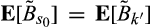


To compute 


 The fundamental matrix (Kao 1996, p. 256) for this Markov chain is


Absorbing States (Indicated by a Thicker Border) when no Action is Taken and Adjusted Yellow Alert Period when
In the absence of any action, (19) reduces to 


Add Ambulances
We assume that 


We modify the Markov chain {(ν(t),w(t)),t ≥ 0} such that 


Modified Markov Chains (Absorbing States have Thicker Borders) when

Expedite Ambulances
We assume that 


We modify the Markov chain {(ν(t),y(t)),t ≥ 0} such that 


Numerical Results and Managerial Insights
In this study, we do not attempt to model the cost of actions, and therefore, we do not suggest optimal actions. Instead, we use our models from section 5 to obtain insights on when EMS staff should take actions, and how these actions compare with each other with respect to the two performance measures, the expected remaining Yellow Alert duration and the expected number of lost calls. We focus on the busiest Calgary segment (τ = 86, with 


When Should Staff Take Actions?
For EMS staff, it is important to understand what would be the implications of waiting, and not taking actions in the hope that the Yellow Alert period will end soon. To gain insights on this question, we keep all parameters related to add and expedite actions fixed and vary the number of busy ambulances at the action epoch, 

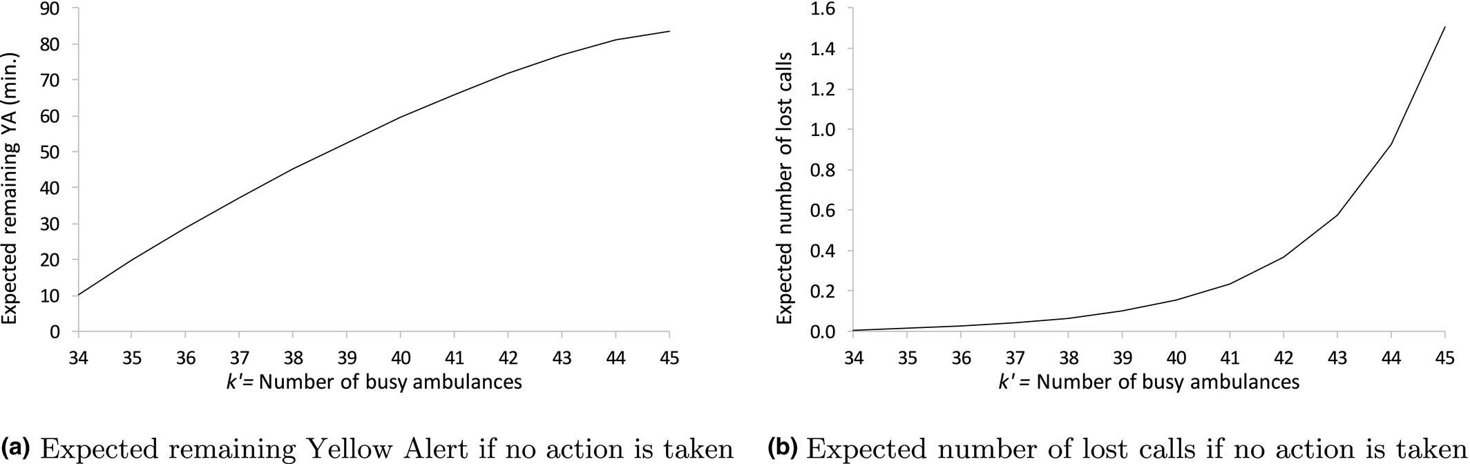
How Performance Measures Escalate when Staff Decide to Wait and Not to Take Actions (Busiest segment, Calgary 2009 Data)
Observation 1: Staff should not wait until a Red Alert to take actions. There is an almost‐linear relationship between 


How Do Actions Compare with Each Other?
Even when staff decide to take an action, the question of “which action should be taken?” is not easy to answer, especially when the expected action realization times (expected action times, for short) are different (that is, 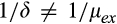
Pairwise Comparison of Actions with Equal Expected Action Times
Adding 


appendix D.4. Consider a special case when 


As discussed in section 1, expediting is realized through actions that lead to a faster transfer of the patient’s care from the EMS to the ED, or to other EMS crews (care consolidation). Adding, however, is realized by borrowing ambulances from neighboring municipalities, from another service (e.g., an interfacility‐transfer ambulance fleet), or asking new ambulance crews to come on duty. Decisions associated with some actions are solely made within the EMS system (e.g., care consolidation), making them easier to manage, but some actions require collaborations with other health care systems (e.g., borrowing ambulances), making them more challenging to manage. Depending on action types, there might be operational difficulties that staff must take into account; for example, neighboring EMS systems may not have available ambulances to lend at a given time.
Observation 2: When 


Comparing


Threshold Values for Comparing Add (


Pairwise Comparison of Actions with Different Expected Action Times
In the same fashion as in Figure , we generated performance curves for 


Table summarizes the largest expected action times that achieve 5% to 50% improvement in the expected remaining Yellow Alert duration of the base case. Table rows show desired improvements in the base case performance measure. For each desired improvement‐action pair in the table, we vary the expected action time between 10 and 60 minutes and record the largest expected action time that satisfies the desired improvement. For example, when 


The Largest Expected Action Time (min.) that Achieves the Target Percentage Improvement in the Expected Remaining Yellow Alert Duration, Compared to the Base Case


The Largest Expected Action Time (min.) that Achieves the Target Percentage Improvement in the Expected Number of Lost Calls, Compared to the Base Case


Observation 3: If staff wait too long before taking action, then the action becomes less effective, even if the expected action time is short. Tables and show that the later an action is taken, the less its marginal improvement in comparison with taking no action becomes, with respect to both performance measures. For example, according to Table , while adding two ambulances can improve the base case up to 30% when 

Expediting, through the consolidation of care of several waiting EMS patients under a single paramedic crew, is perhaps the action that requires the least coordination with other agencies, and therefore could be realized quickly. Here, we provide more insights on this action by comparing expediting 


Observation 4: When 


The Largest Expected Action Time (min.) for Expediting 2 Ambulance that Outperforms Adding 1 Ambulance that is Available Instantaneously, with Respect to the Expected Number of Lost Calls

The Largest Expected Action Time (min.) for Expediting 2 Ambulance that Outperforms Adding 1 Ambulance that is Available Instantaneously, with Respect to the Expected Remaining Yellow Alert Duration

Conclusion
This study provides an understanding of capacity shortage periods in mission critical systems like fire, police, and EMS. We focus on EMS systems and model these systems as Erlang loss systems with service times modeled as either Markovian and state‐dependent (M(k)) or general (G). We show that the expected duration of periods during which at least k out of c ambulances are busy is independent of the shape of the service time distribution beyond its mean, but this is not true of the higher moments. We obtain closed‐form formulas and easy‐to‐use recursions to calculate the expected duration and (for M(k) service times) the standard deviation of ambulance‐shortage periods. We validate our formulas for the mean and standard deviation of partial busy periods against empirical data from the Calgary and Edmonton EMS systems. Our validation results show that although ambulance service times are far from exponential, the loss model with Markovian state‐dependent service time slightly outperforms the loss model with general service time, with respect to predicting the first moment of partial busy periods.
We expand the M/M(k)/c/c model and use the theory of absorbing Markov chains to quantify the impact of adding or expediting ambulances on two performance measures: The expected remaining duration of a Yellow Alert (a proxy for periods with long response times) and the expected number of lost calls during this residual duration. We show that, regardless of the action type, the expected number of lost calls increases rapidly when the number of available ambulances at action epoch decreases, and that the escalation is almost linear with respect to the other performance measure. Based on our results, both performance measures are monotonic functions of the expected value of the time until actions are realized (1/δ and 
Several related issues could benefit from further study, including: models and algorithms to choose the Yellow Alert threshold θ so as to balance mitigation of capacity shortages and the added workload from operating in alert mode; investigating whether θ should vary with time; investigating the action of delaying response to low‐priority calls during alert periods; analytically investigating when the stationary approach, as opposed to the transient approach, works well in modeling loss systems and providing simple modifications for improvements, if needed; and empirically investigating whether the time required to expedite (add) one additional ambulance becomes progressively larger, as one would expect.
Footnotes
Acknowledgments
The authors thank the Department Editor, Associate Editor, and three anonymous referees for their thoughtful comments that led to considerable improvements in this study. We are also grateful to Alberta Health Services (AHS) for providing the data and to AHS staff for their empirical insights. This work was partially supported by the Canadian Natural Science and Engineering Research Council (Discovery Grant 203534).
1
Protocols that define when a Yellow Alert is triggered sometimes include additional considerations besides the number of available units, such as “7 or fewer units … sustained for 15 minutes.” We use alert period definitions that are solely based on the number of available units, for simplicity.