Context‐based dynamic pricing with online clustering

Abstract

We consider a context‐based dynamic pricing problem of online products, which have low sales. Sales data from Alibaba, a major global online retailer, illustrate the prevalence of low‐sale products. For these products, existing single‐product dynamic pricing algorithms do not work well due to insufficient data samples. To address this challenge, we propose pricing policies that concurrently perform clustering over product demand and set individual pricing decisions on the fly. By clustering data and identifying products that have similar demand patterns, we utilize sales data from products within the same cluster to improve demand estimation for better pricing decisions. We evaluate the algorithms using regret, and the result shows that when product demand functions come from multiple clusters, our algorithms significantly outperform traditional single‐product pricing policies. Numerical experiments using a real data set from Alibaba demonstrate that the proposed policies, compared with several benchmark policies, increase the revenue. The results show that online clustering is an effective approach to tackling dynamic pricing problems associated with low‐sale products.

Keywords

dynamic pricing low‐sale product online clustering regret analysis

INTRODUCTION

Over the past several decades, dynamic pricing has been widely adopted by industries, such as retail, airlines, and hotels, with great success (see, e.g., Cross, 1995; Smith et al., 1992). Dynamic pricing has been recognized as an important lever not only for balancing supply and demand, but also for increasing revenue and profit. Recent advances in online retailing and increased availability of online sales data have created opportunities for firms to better use customer information to make pricing decisions, see, for example, the survey paper by den Boer (2015). Indeed, the advances in information technology have made the sales data easily accessible, facilitating the estimation of demand and the adjustment of price in real time. Increasing availability of demand data allows for more knowledge to be gained about the market and customers, as well as the use of advanced analytics tools to make better pricing decisions.

However, in practice, there are often products with low sales amount or user views. For these products, few available data points exist. For example, Tmall Supermarket, a business division of Alibaba, is a large‐scale online store. In contrast to a typical consumer‐to‐consumer (C2C) platform (e.g., Taobao under Alibaba) that has millions of products available, Tmall Supermarket is designed to provide carefully selected high‐quality products to customers. We reviewed the sales data from May to July of 2018 on Tmall Supermarket with nearly 75,000 products offered during this period of time, and they show that more than 16,000 products (21.6% of all products) have a daily average number of unique visitors (UVs)¹ less than 10, and more than 10,000 products (14.3% of all products) have a daily average number of UVs at most 1. Although each low‐sale product alone may have little impact on the company's revenue, the combined sales of all low‐sale products are significant.

Pricing low‐sale products is often challenging due to the limited sales records available for demand estimation. In fast‐evolving markets (e.g., fashion or online advertising), demand data from the distant past may not be useful for predicting customers' purchasing behavior in the near future. Classical statistical estimation theory has shown that data insufficiency leads to large estimation error of the underlying demand, which results in suboptimal pricing decisions. To overcome the issue of data insufficiency, some literature in other applications such as customer segmentation cluster the objects (i.e., customers) using their feature data (see, e.g., Su & Chen, 2015). However, clustering low‐sale products by their features may not always work well. For the following two reasons, in this paper we choose to define clusters based on demand patterns rather than features for low‐sale products: (i) Some products with very similar features may have very different demand, for example, two bags with same/similar appearance may have totally different demand because one belongs to a famous brand and the other is a copycat (only difference is the feature of product brand). (ii) Some (seemingly) completely unrelated products may exhibit same or similar demand pattern. In fact, the research on dynamic pricing of products with little sales data remains relatively unexplored. To the best of our knowledge, there exists no dynamic pricing policy in the literature for low‐sale products that admits theoretical performance guarantee. This paper fills the gap by developing adaptive context‐based dynamic pricing learning algorithms for low‐sale products, and our results show that the algorithms perform well both theoretically and numerically.

Contributions of this paper

Although each low‐sale product only has a few sales records, the total number of low‐sale products is usually quite large. In this paper, we address the challenge of pricing low‐sale products using an important idea from machine learning—clustering. Our starting point is that there are some set of products out there, though we do not know which ones, that share similar underlying demand patterns. For these products, information can be extracted from their collective sales data to improve the estimation of their demand function. The problem is formulated as developing adaptive learning algorithms that identify the products exhibiting similar demand patterns, and extract the hidden information from sales data of seemingly unrelated products to improve the pricing decisions of low‐sale products and increase revenue. As we mentioned earlier in the introduction, our method of clustering is based on similar demand patterns instead of similar product features. The reason is that products with similar features may have different demand.

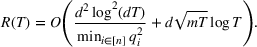
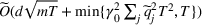
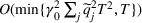
We consider a generalized linear demand model with arbitrary contextual covariate information about products and develop a learning algorithm that integrates product clustering with pricing decisions. Our policy consists of two phases. The first phase constructs confidence bounds on the distance between clusters, which enables dynamic clustering without any prior knowledge of the cluster structure. The second phase carefully controls the price variation based on the estimated clusters, striking a proper balance between price exploration and revenue maximization by exploiting the cluster structure. Since the pricing part of the algorithm is inspired by semimyopic policy proposed by Keskin and Zeevi (2014), we refer to our algorithm as the Clustered Semi‐Myopic Pricing (CSMP) policy. We first establish the theoretical regret bound of the proposed policy. Specifically, when the demand functions of the products belong to m clusters, where m is smaller than the total number of products (denoted by n), the performance of our algorithm is better than that of existing dynamic pricing policies that treat each product separately. Let T denote the length of the selling season; we show in Theorem 1 that our algorithm achieves the regret of

\tilde{O} (\sqrt{m T})

, where

\tilde{O} (\cdot)

hides the logarithmic terms. This result, when m is much smaller than n, is a significant improvement over the regret when applying a single‐product pricing policy to individual products, which is typically

\tilde{O} (\sqrt{n T})

We carry out a thorough numerical experiment using both synthetic data and a real data set from Alibaba consisting of a large number of low‐sale products. Several benchmarks, one treats each product separately, one puts all products into a single cluster, and the other one applies a classical clustering method (K‐means method for illustration), are compared with our algorithms under various scenarios. The numerical results show that our algorithms are effective and their performances are consistent in different scenarios (e.g., with almost static covariates, model misspecification).

It is well known that providing a performance guarantee for a clustering method is challenging due to the nonconvexity of the loss function (e.g., in K‐means), which is why there exists no clustering and pricing policy with theoretical guarantees in the existing literature. This is the first paper to establish the regret bound for a dynamic clustering and pricing policy. Instead of adopting an existing clustering algorithm from the machine learning literature (e.g., K‐means), which usually requires the number of clusters as an input, our algorithms dynamically update the clusters based on the gathered information about customers' purchase behavior. In addition to significantly improving the theoretical performance as compared to classical dynamic pricing algorithms without clustering, our algorithms demonstrate excellent performance in our simulation study.

Literature review

In this subsection, we review some related research from both the revenue management and machine learning literature.

Related literature in dynamic pricing

Due to increasing popularity of online retailing, dynamic pricing has become an active research area in revenue management in the past decade. We only briefly review a few of the most related works and refer the interested readers to den Boer (2015) and Kumar et al. (2018) for comprehensive literature surveys. Earlier work and review of dynamic pricing include Bitran and Caldentey (2003), Elmaghraby and Keskinocak (2003), Gallego and Van Ryzin (1994), and Gallego and Van Ryzin (1997). These papers assume that demand information is known to the retailer a priori and either characterize or compute the optimal pricing decisions. In some retailing industries, such as fast fashion, this assumption may not hold due to the quickly changing market environment. As a result, with the recent development of information technology, combining dynamic pricing with demand learning has attracted much interest in research. Depending on the structure of the underlying demand functions, these works can be roughly divided into two categories: parametric demand models (see, e.g., Bertsimas & Perakis, 2006; Besbes & Zeevi, 2009; Broder & Rusmevichientong, 2012; Carvalho & Puterman, 2005; Chen, Simchi‐Levi, et al., 2022; den Boer & Zwart, 2013; Farias & Van Roy, 2010; Harrison et al., 2012; Keskin & Zeevi, 2014; Wang et al., 2021) and nonparametric demand models (see, e.g., Araman & Caldentey, 2009; Besbes & Zeevi, 2015; Chen et al., 2015, 2021; Chen & Shi, 2019; Chen & Wang, 2022; Cheung et al., 2017; Cohen et al., 2018; Lei et al., 2014; Wang et al., 2014). The aforementioned papers assume that the price is continuous. Other works consider a discrete set of prices, see, for example, Ferreira et al. (2018), and recent studies examine pricing problems with strategic customers (e.g., Chen, Gao, et al., 2022) or in dynamically changing environments (e.g., Besbes et al., 2015; Keskin & Zeevi, 2016)

Dynamic pricing and learning with demand covariates (or contextual information) have received increasing attention in recent years because of their flexibility and clarity in modeling customers and market environment. Research involving this information include, among others, Ban and Keskin (2021), Chen, Owen, et al. (2022), Chen and Gallego (2021), Javanmard and Nazerzadeh (2019), Lobel et al. (2018), Nambiar et al. (2019), and Qiang and Bayati (2016). In many online‐retailing applications, sellers have access to rich covariate information reflecting the current market situation. Moreover, the covariate information is not static but usually evolves over time. Our paper incorporates time‐evolving covariate information into the demand model. In particular, given the observable covariate information of a product, we assume that the customer decision depends on both the selling price and covariates. Although covariates provide richer information for accurate demand estimation, a demand model that incorporates covariate information involves more parameters to be estimated. Therefore, it requires more data for estimation with the presence of covariates, which poses an additional challenge for low‐sale products.

Related literature in clustering for pricing

In the literature, there are some interesting two‐stage methods that first use historical data to determine the cluster structure of demand functions in an offline manner, and then dynamically make pricing decisions for another product by learning which cluster it demand belongs to. Ferreira et al. (2015) study a pricing problem with flash sales on the Rue La La platform. Using historical information and offline optimization, the authors classify the demand of all products into multiple groups, and use demand information for products that did not experience lost sales to estimate demand for products that had lost sales. They construct “demand curves” on the percentage of total sales with respect to the number of hours after the sales event starts, then classify these curves into four clusters. For a sold‐out product, they check which one of the four curves is the closest to its sales behavior and use that to estimate the lost sales. Cheung et al. (2017) consider the single‐product pricing problem, where the demand of the product is assumed to be from one of the K demand functions (called demand hypothesis in that paper). Those K demand functions are assumed to be known, and the decision is to choose which of those functions is the true demand curve of the product. In their field experiment with Groupon, they applied K‐means clustering to historical demand data to generate those K demand functions offline. That is, clustering is conducted offline first using historical data, then dynamic pricing decisions are made in an online fashion for a new product, assuming that its demand is one of the K demand functions. Very recently, Keskin et al. (2020) studied personalized pricing in retail electricity market, where they applied a spectral clustering approach to decide customer types based on customers' features. In this paper, as we discussed earlier, instead of using observable features, we cluster products based on estimated demand patterns.

Related literature in clustering

We end this section by giving a brief overview of clustering methods in the machine learning literature. To save space, we only discuss several popular clustering methods, and refer the interested reader to Saxena et al. (2017) for a recent literature review on the topic. The first one is called hierarchical clustering (Murtagh, 1983), which iteratively clusters objects (either bottom‐up, from a single object to several big clusters; or top‐down, from a big cluster to single product). Comparable with hierarchical clustering, another class of clustering method is partitional clustering, in which the objects do not have any hierarchical structure, but rather are grouped into different clusters horizontally. Among these clustering methods, K‐means clustering is probably the most well‐known and most widely applied method (see, e.g., MacQueen et al., 1967). Several extensions and modifications of K‐means clustering method have been proposed in the literature, for example, K‐means++ (Arthur & Vassilvitskii, 2007) and fuzzy c‐means clustering (Dunn, 1973). Another important class of clustering method is based on graph theory. For instance, the spectral clustering uses graph Laplacian to help determine clusters (Shi & Malik, 2000; Von Luxburg, 2007). Beside these general methods for clustering, there are many clustering methods for specific problems such as decision tree, neural network, etc. It should be noted that nearly all the clustering methods in the literature are based on offline data. This paper, however, integrates clustering into online learning and decision‐making process.

Organization of the paper

The remainder of this paper is organized as follows. In Section 2, we present the problem formulation. Our main algorithm is presented in Section 3 together with the theoretical results for the algorithm performance. In Section 4, we report the results of several numerical experiments based on both synthetic data and a real data set. We conclude the paper with a discussion about future research in Section 5. Finally, all the technical proofs are presented in the Supporting Information.

PROBLEM FORMULATION

We consider a retailer that sells n products, labeled by

i = 1, 2, …, n

, with unlimited inventory (e.g., there is an inventory replenishment scheme such that products typically do not run out of stock). Following the literature, we denote the set of these products by [n]. We mainly focus on online retailing of low‐sale products. These products are typically not offered to customers as a display; hence we do not consider substitutability/complementarity of products in our model. Furthermore, these products are usually not recommended by the retailer on the platform, and instead, customers search to view them online. We let

q_{i} > 0

denote the percentage of potential customers who are interested in, or view/search for, product

i \in [n]

. In this paper, we will treat

q_{i}

as the probability an arriving customer views product i; in another word,

q_{i}

can be considered as the arrival rate of customers viewing product i, which are independent from each other.

Customers arrive sequentially at time

t = 1, 2, …, T

, and we denote the set of all time indices by [T]. For simplicity, we assume without loss of generality that there is exactly one arrival during each period. In each time period t, the firm first observes some covariates for each product i, such as product rating, prices of competitors, average sales in past few weeks, and promotion‐related information (e.g., whether the product is currently on sale). We denote the covariates of product i by

z_{i, t} \in R^{d}

, where d is the dimension of the covariates that is usually small (as compared to n or T). The covariates

z_{i, t}

change over time and satisfy

| | z_{i, t} {| |}_{2} \leq 1

after normalization. Then, the retailer sets the price

p_{i, t} \in [\underset{̲}{p}, \bar{p}]

for each product i, where

0 \leq \underset{̲}{p} < \bar{p} < \infty

(the assumption of the same price range for all products is without loss of generality). Let

i_{t}

denote the product that the customer searches in period t (or customer t). After observing the price and other details of product

i_{t}

, customer t then decides whether or not to purchase it. The sequence of events in period t is summarized as follows:

(i)
In time t, the retailer observes the covariates
$z_{i, t}$
for each product
$i \in [n]$
, then sets the price
$p_{i, t}$
for each
$i \in [n]$
.
(ii)
Customer searches for product
$i_{t} \in [n]$
in period t with probability
$q_{i_{t}}$
independent of others and then observes its price
$p_{i_{t}, t}$
.
(iii)
The customer decides whether or not to purchase product
$i_{t}$
.

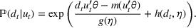
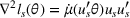
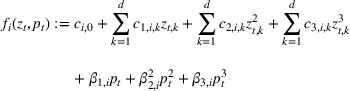
The customer's purchasing decision follows a GLM (see, e.g., McCullagh & Nelder, 1989). That is, given price
$p_{i_{t}, t}$
of product
$i_{t}$
at time t, the customer's purchase decision is represented by a Bernoulli random variable
$d_{i_{t}, t} (p_{i_{t}, t}; z_{i_{t}, t}) \in {0, 1}$
, where
$d_{i_{t}, t} (p_{i_{t}, t}; z_{i_{t}, t}) = 1$
if the customer purchases product
$i_{t}$
and 0 otherwise. The purchase probability, which is the expectation of
$d_{i_{t}, t} (p_{i_{t}, t}; z_{i_{t}, t})$
, takes the form
$E [d_{i_{t}, t} (p_{i_{t}, t}; z_{i_{t}, t})] = μ (α_{i_{t}}^{'} x_{i_{t}, t} + β_{i_{t}} p_{i_{t}, t}),$
1
where
$μ (\cdot)$
is the link function,
$x_{i_{t}, t}^{'} = (1, z_{i_{t}, t}^{'})$
is the corresponding extended demand covariate with the 1 in the first entry used to model the bias term in a GLM model, and the expectation is taken with respect to customer purchasing decision. Let
$θ_{i_{t}}^{'} = (α_{i_{t}}^{'}, β_{i_{t}})$
be the unknown parameter of product
$i_{t}$
, which is assumed to be bounded. That is,
$| | θ_{i} {| |}_{2} \leq L$
for some constant L for all
$i \in [n]$
. Remark 1
The commonly used linear and logistic models are special cases of GLM with link function
$μ (x) = x$
and
$μ (x) = \exp (x) / (1 + \exp (x))$
, respectively. The parametric demand model (1) has been used in a number of papers on pricing with contextual information, see, for example, Qiang and Bayati (2016) (for a special case of linear demand with
$μ (x) = x$
) and Ban and Keskin (2021).

For convenience and with a slight abuse of notation, we write
$p_{t} : = p_{i_{t}, t}, z_{t} : = z_{i_{t}, t}, x_{t} : = x_{i_{t}, t}, d_{t} : = d_{i_{t}, t},$
2
where “:=” stands for “defined as.” Let the feasible sets of
$x_{t}$
and
$θ_{i}$
be denoted as
$X$
and Θ, respectively. We further define
$T_{i, t} : = {s \leq t : i_{s} = i}$
3
as the set of time periods before t in which product i is viewed, and
$T_{i, t} : = | T_{i, t} |$
its cardinality. With this demand model, the expected revenue
$r_{t} (p_{t})$
of each round t is
$\begin{matrix} r_{t} (p_{t}) : = p_{t} μ (α_{i_{t}}^{'} x_{t} + β_{i_{t}} p_{t}) . \end{matrix}$
4
Note that we have made the dependency of
$r_{t} (p_{t})$
on
$x_{t}$
implicit.

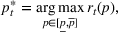
The firm's optimization problem and regret

The firm's goal is to decide the price
$p_{t} \in [\underset{̲}{p}, \bar{p}]$
at each time t for each product to maximize the cumulative expected revenue
$\sum_{t = 1}^{T} E [r_{t} (p_{t})]$
, where the expectation is taken with respect to the randomness of the pricing policy as well as the stream of
$i_{t}$
for
$t \in [T]$
, and for the next section, also the stochasticity in contextual covariates
$z_{t}$
,
$t \in [T]$
. The goal of maximizing the expected cumulative revenue is equivalent to minimizing the so‐called regret, which is defined as the revenue gap as compared with the clairvoyant decision maker who knew the underlying parameters in the demand model a priori. With the known demand model, the optimal price can be computed as
$p_{t}^{} = \underset{p \in [\underset{̲}{p}, \bar{p}]}{arg max} r_{t} (p),$
5
and the corresponding revenue gap at time t is
$E [r_{t} (p_{t}^{}) - r_{t} (p_{t})]$
(the dependency of
$p_{t}^{}$
on
$x_{t}$
is again made implicit). The cumulative regret of a policy π with prices
${p_{t}}_{t = 1}^{T}$
is defined by the summation of revenue gaps over the entire time horizon, that is,
$R^{π} (T) : = \sum_{t = 1}^{T} E [r_{t} (p_{t}^{}) - r_{t} (p_{t})] .$
6
Remark 2
For consistency with the online pricing literature, see, for example, Ban and Keskin (2021), Chen, Owen, et al. (2022), Javanmard and Nazerzadeh (2019), and Qiang and Bayati (2016), in this paper we use expected revenue as the objective to maximize. However, we point out that all our analyses and results carry over to the objective of profit maximization. That is, if
$c_{t}$
is the cost of the product in round t, then the expected profit in (4) can be replaced by
$r_{t} (p_{t}) = (p_{t} - c_{t}) μ (α_{i_{t}}^{'} x_{t} + β_{i_{t}} p_{t}) .$
7

Cluster of products

Two products i₁ and i₂ are said to be “similar” if they have similar underlying demand functions, that is,
$θ_{i_{1}}$
and
$θ_{i_{2}}$
are close. In this paper, we assume that the n products can be partitioned into m clusters,
$N_{j}$
for
$j = 1, 2, …, m$
, such that for arbitrary two products i₁ and i₂, we have
$θ_{i_{1}} = θ_{i_{2}}$
if i₁ and i₂ belong to the same cluster; otherwise,
$| | θ_{i_{1}} - θ_{i_{2}} {| |}_{2} \geq γ > 0$
for some constant γ. We refer to this cluster structure as the γ‐gap assumption, which will be relaxed in Remark 7 of Section 3.2. For convenience, we denote the set of clusters by [m], and by a bit abuse of notation, let
$N_{i}$
be the cluster to which product i belongs.

It is important to note that the number of clusters m and each cluster
$N_{j}$
are unknown to the decision maker a priori. Indeed, in some applications, such structure may not exist at all. If such a structure does exist, then our policy can identify such a cluster structure and make use of it to improve the practical performance and the regret bound. However, we point out that the cluster structure is not a requirement for the pricing policy to be discussed. In other words, our policy reduces to a standard dynamic pricing algorithm when demand functions of the products are all different (i.e., when
$m = n$
).

It is also worthwhile to note that our clustering is based on demand parameters/patterns and not on product categories or features, since it is the demand of the products that we want to learn. The clustering approach based on demand is prevalent in the literature (besides Cheung et al., 2017; Ferreira et al., 2015, and the references therein, we also refer to Van Kampen et al., 2012, for a comprehensive review). Clustering based on category/feature similarity is useful in some problems (see, e.g., Su & Chen, 2015, investigate customer segmentation using features of clicking data), but it does not apply to our setting because, for instance, products with similar feature for different brands may have very different demand (see our earlier discussion in the introduction). Moreover, in our model, motivated by Alibaba's business the product feature
$x_{i, t}$
is non‐stationary, so feature‐based clustering can lead to different clusters in different time. Remark 3
For its application to the online pricing problem, the contextual information in our model is about the product. That is, at the beginning of each period, the firm observes the contextual information about each product, then determines the pricing decision for the product, and then the arriving customer makes a purchasing decision. We point out that our algorithm and result apply equally to personalized pricing in which the contextual information is about the customer. That is, a customer arrives (e.g., logging on the website) and reveals his/her contextual information, and then the firm makes a pricing decision based on that information. The objective is to make personalized pricing decisions to maximize total revenue (see, e.g., Ban & Keskin, 2021).

PRICING POLICY AND MAIN RESULTS

In this section, we discuss the specifics of the learning algorithm, its theoretical performance, and a sketch of its proof. Specifically, we describe the policy procedure and discuss its intuitions in Section 3.1 before presenting its regret and outlining the proof in Section 3.2.

Description of the pricing policy

Our policy consists of two phases for each period
$t \in [T]$
: The first phase constructs a neighborhood for each product
$i \in [n]$
, and the second phase determines its selling price. In the first step, our policy uses individual data of each product
$i \in [n]$
to estimate parameters
${\hat{θ}}_{i, t - 1}$
. This estimation is used only for construction of the neighborhood
${\hat{N}}_{i, t}$
for product i. Once the neighborhood is defined, we consider all the products in this neighborhood as in the same cluster and use clustered data to estimate the parameter vector
${\tilde{θ}}_{{\hat{N}}_{i, t}, t - 1}$
. The latter is used in computing the selling price of product i. We refer to Figure 1 for a flowchart of our policy, and present the detailed procedure in Algorithm 1.

FIGURE 1
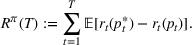
Flow chart of the algorithm
ALGORITHM 1
The CSMP Algorithm

Require: c, the confidence bound parameter; Δ₀, price perturbation parameter;

1: Step 0. Initialization. Initialize $T_{i, 0} = \emptyset$ and
$V_{i, 0} = I$
for all
$i \in [n]$
. Let
$t = 1$
and go to Step 1.

2: for
$t = 1, 2, …, T$
do

3:
Step 1. Individual Parametric Estimation. Compute the MLE using individual data

${\hat{θ}}_{i, t - 1} = {arg min}_{θ \in Θ} \sum_{s \in T_{i, t - 1}} l_{s} (θ)$

for all
$i \in [n]$
. Go to Step 2.

4:
Step 2. Neighborhood Construction. Compute the neighborhood of each product i as

${\hat{N}}_{i, t} = {i^{'} \in [n] : | | {\hat{θ}}_{i^{'}, t - 1} - {\hat{θ}}_{i, t - 1} {| |}_{2} \leq B_{i^{'}, t - 1} + B_{i, t - 1}}$

where
$B_{i, t - 1}$
is defined in (12) for each
$i \in [n]$
. Go to Step 3.

5:
Step 3. Clustered Parametric Estimation. Compute the MLE using clustered data

${({\tilde{α}}_{{\hat{N}}_{i, t}, t - 1}^{'}, {\tilde{β}}_{{\hat{N}}_{i, t}, t - 1})}^{'} = {\tilde{θ}}_{{\hat{N}}_{i, t}, t - 1} = {arg min}_{θ \in Θ} \sum_{s \in {\tilde{T}}_{{\hat{N}}_{i, t}, t - 1}} l_{s} (θ)$

for each
$i \in [n]$
. Go to Step 4.

6:
Step 4. Pricing. Compute price for each
$i \in [n]$
as

$p_{i, t}^{'} = {arg max}_{p \in [\underset{̲}{p}, \bar{p}]} μ (α_{{\hat{N}}_{i, t}, t - 1}^{'} x_{i, t} + β_{{\hat{N}}_{i, t}, t - 1} p) p,$

then project to
${\tilde{p}}_{i, t} = {Proj}_{[\underset{̲}{p} + | Δ_{i, t} |, \bar{p} - | Δ_{i, t} |]} (p_{i, t}^{'})$
and offer to the customer price
$p_{i, t} = {\tilde{p}}_{i, t} + Δ_{i, t}$
where
$Δ_{i, t} = \pm Δ_{0} {\tilde{T}}_{{\hat{N}}_{i, t}, t}^{- 1 / 4}$
which takes two signs with equal probability.

7: Then, customer t arrives, searches for product
$i_{t}$
, and makes purchasing decision
$d_{i_{t}, t} (p_{i_{t}, t}; z_{i_{t}, t})$
. Update
$T_{i_{t}, t} = T_{i_{t}, t - 1} \cup {t}$
and
$V_{i_{t}, t} = V_{i_{t}, t - 1} + u_{t} u_{t}^{'}$
.

8: end for

In the following, we discuss the parameter estimation of GLM demand functions and the construction of a neighborhood in detail.

Parameter estimation of GLM

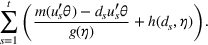
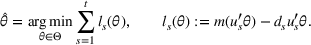
As shown in Figure 1, the parameter estimation is an important part of our policy construction. We adopt the classical maximum likelihood estimation (MLE) method for parameter estimation (see McCullagh & Nelder, 1989). For completeness, we briefly describe the MLE method here. Let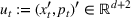
$u_{t} : = {(x_{t}^{'}, p_{t})}^{'} \in R^{d + 2}$
. The conditional distribution of the demand realization
$d_{t}$
, given
$u_{t}$
, belongs to the exponential family and can be written as
$P (d_{t} | u_{t}) = \exp (\frac{d_{t} u_{t}^{'} θ - m (u_{t}^{'} θ)}{g (η)} + h (d_{t}, η)) .$
8
Here
$m (\cdot), g (\cdot)$
, and
$h (\cdot)$
are some specific functions, where
$\dot{m} (u_{t}^{'} θ) = E [d_{t}] = μ (u_{t}^{'} θ)$
depends on
$μ (\cdot)$
and
$h (d_{t}, η)$
is the normalization part, and η is some known scale parameter. Suppose that we have t samples
$(d_{s}, p_{s})$
for
$s = 1, 2, …, t$
, the negative log‐likelihood function of θ under model (8) is
$\sum_{s = 1}^{t} (\frac{m (u_{s}^{'} θ) - d_{s} u_{s}^{'} θ}{g (η)} + h (d_{s}, η)) .$
9
By extracting the terms in (9) that involves θ, the maximum likelihood estimator
$\hat{θ}$
is
$\hat{θ} = \underset{θ \in Θ}{arg min} \sum_{s = 1}^{t} l_{s} (θ), l_{s} (θ) : = m (u_{s}^{'} θ) - d_{s} u_{s}^{'} θ .$
10
Since
$\nabla^{2} l_{s} (θ) = \dot{μ} (u_{s}^{'} θ) u_{s} u_{s}^{'}$
is positive semidefinite in a standard GLM model (by Assumption A‐2 in the next subsection), the optimization problem in (10) is convex and can be easily solved.

Determining the neighborhood of each product

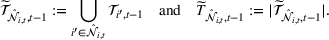
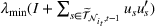
The first phase of our policy determines which products to include in the neighborhood of each product
$i \in [n]$
. We use the term “neighborhood” instead of cluster, though closely related, because clusters are usually assumed to be disjoint in the machine learning literature. In contrast, by our definition of neighborhood, some products can belong to different neighborhoods depending on the estimated parameters. To define the neighborhood of i, which is denoted by
${\hat{N}}_{i, t}$
, we first estimate parameter
${\hat{θ}}_{i, t - 1}$
of each product
$i \in [n]$
using their own data, that is,
${\hat{θ}}_{i, t - 1}$
is the maximum likelihood estimator using data in
$T_{i, t - 1}$
defined in (3). Then, we include a product
$i^{'} \in [n]$
in the neighborhood
${\hat{N}}_{i, t}$
of i if their estimated parameters are sufficiently close, which is defined as
$| | {\hat{θ}}_{i^{'}, t - 1} - {\hat{θ}}_{i, t - 1} {| |}_{2} \leq B_{i^{'}, t - 1} + B_{i, t - 1},$
11
where
$B_{i, t - 1}$
is a confidence bound for product i given by
$B_{i, t} : = \frac{\sqrt{c (d + 2) \log (1 + t)}}{\sqrt{λ_{\min} (V_{i, t})}} .$
12
Here,
$V_{i, t} : = I + \sum_{s \in T_{i, t}} u_{s} u_{s}^{'}$
is the empirical Fisher's information matrix of product
$i \in [n]$
at time t and c is some positive constant, which will be specified in our theory development. Note that, by the γ‐gap assumption discussed at the end of Section 2, the method will work even when
$T_{i, t - 1}$
only contains a limited number of sales records.

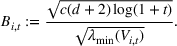
Setting the price of each product

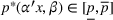
Once we define the (estimated) neighborhood
${\hat{N}}_{i, t}$
of
$i \in [n]$
, we can pool the demand data of all products in
${\hat{N}}_{i, t}$
to learn the parameter vector. That is, we let
${\tilde{T}}_{{\hat{N}}_{i, t}, t - 1} : = ⋃_{i^{'} \in {\hat{N}}_{i, t}} T_{i^{'}, t - 1} and {\tilde{T}}_{{\hat{N}}_{i, t}, t - 1} : = | {\tilde{T}}_{{\hat{N}}_{i, t}, t - 1} | .$
13
The clustered parameter vector
${\tilde{θ}}_{{\hat{N}}_{i, t}, t - 1}$
is the maximum likelihood estimator using data in
${\tilde{T}}_{{\hat{N}}_{i, t}, t - 1}$
.

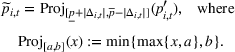
To decide on the price, we first compute
$p_{i, t}^{'}$
, which is the “optimal price” based on the estimated clustered parameters
${\tilde{θ}}_{{\hat{N}}_{i, t}, t - 1}$
. Then we restrict
$p_{i, t}^{'}$
to the interval
$[\underset{̲}{p} + | Δ_{i, t} |, \bar{p} - | Δ_{i, t} |]$
by the projection operator. That is, we compute
$\begin{matrix} {\tilde{p}}_{i, t} = {Proj}_{[\underset{̲}{p} + | Δ_{i, t} |, \bar{p} - | Δ_{i, t} |]} (p_{i, t}^{'}), where \\ {Proj}_{[a, b]} (x) : = \min {\max {x, a}, b} . \end{matrix}$
14
The reasoning for this restriction is that our final price
$p_{i, t}$
will be
$p_{i, t} = {\tilde{p}}_{i, t} + Δ_{i, t}$
, and the projection operator forces the final price
$p_{i, t}$
to the range
$[\underset{̲}{p}, \bar{p}]$
. Here, the price perturbation
$Δ_{i, t} = \pm Δ_{0} {\tilde{T}}_{{\hat{N}}_{i, t}, t}^{- 1 / 4}$
takes a positive or a negative value with equal probability, where Δ₀ is a positive constant. We add this price perturbation for the purpose of price exploration. Intuitively, the more price variation we have, the more accurate the parameter estimation will be. However, too much price variation leads to loss of revenue because we deliberately charged a “wrong” price. Therefore, it is crucial to find a balance between these two targets by defining an appropriate
$Δ_{i, t}$
.

We note that this pricing scheme belongs to the class of semimyopic pricing (SMP) policies defined in Keskin and Zeevi (2014). Since our policy combines clustering with SMP, we refer to it as the CSMP algorithm.

We briefly discuss each step of the algorithm and the intuition behind the theoretical performance. For Steps 1 and 2, the main purpose is to identify the correct neighborhood of the product searched in period t; that is,
${\hat{N}}_{i_{t}, t} = N_{i_{t}}$
with high probability (for brevity of notation, we let
${\hat{N}}_{t} : = {\hat{N}}_{i_{t}, t}$
). To achieve that, two conditions are necessary. First, the estimator
${\hat{θ}}_{i, t}$
should converge to
$θ_{i}$
as t grows for all
$i \in [n]$
. Second, the confidence bound
$B_{i, t}$
should converge to 0 as t grows, such that in Step 2, we are able to identify different neighborhood by the γ‐gap assumption among clusters. To satisfy these conditions, classical statistical learning theory (see, e.g., Lemma EC.2 in the Supporting Information) requires the minimum eigenvalue of the empirical Fisher's information matrix
$V_{i, t}$
to be sufficiently above zero, or more specifically,
$λ_{\min} (V_{i, t}) \geq Ω (q_{i} \sqrt{t})$
(see Lemma EC.3 in the Supporting Information). This requirement is guaranteed by the variation assumption on demand covariates
$x_{i, t}$
, which will be imposed in Assumption A‐3 in the next subsection, plus our choice of price perturbation in Step 4.

Following the discussion above, when
${\hat{N}}_{t} = N_{i_{t}}$
with high probability, we can cluster the data within
$N_{i_{t}}$
to increase the number of samples for
$i_{t}$
. Because of the increased data samples, it is expected that the estimator
${\tilde{θ}}_{N_{i_{t}}, t - 1}$
for
$θ_{i_{t}}$
in Step 3 is more accurate than
${\hat{θ}}_{i, t - 1}$
. Of course, the estimation accuracy again requires the minimum eigenvalue of the empirical Fisher's information matrix over the clustered set
${\tilde{T}}_{N_{i_{t}}, t - 1}$
, that is,
$λ_{\min} (I + \sum_{s \in {\tilde{T}}_{N_{i_{t}}, t - 1}} u_{s} u_{s}^{'})$
, to be sufficiently large, which is again guaranteed by stochastic assumption of
$z_{i, t}$
and the price perturbation in Step 4.

The design of the CSMP algorithm depends critically on two things. First, by taking an appropriate price perturbation in Step 4, we balance the exploration and exploitation. If the perturbation is too much, even though it helps to achieve good parameter estimation, it may lead to loss of revenue (due to purposely charging the wrong price). Second, the sequence of demand covariates
$z_{i, t}$
has to satisfy an important variation assumption (Assumption A‐3). Later we will see that this variation assumption is weaker than the typical stochastic assumption on
$z_{i, t}$
, which is commonly seen in the pricing literature with demand covariates (see, e.g., Ban & Keskin, 2021; Chen, Owen, et al., 2022; Javanmard & Nazerzadeh, 2019; Qiang & Bayati, 2016).

Theoretical performance of the CSMP algorithm

This section presents the regret of the CSMP pricing policy. Before proceeding to the main result, we first make some technical assumptions that will be needed for the theorem. Assumption A
1.
The expected revenue function
$p μ (α^{'} x + β p)$
has a unique maximizer
$p^{*} (α^{'} x, β) \in [\underset{̲}{p}, \bar{p}]$
, which is Lipschitz in
$(α^{'} x, β)$
with parameter L₀ for all
$x \in X$
and
$θ \in Θ$
. Moreover, the unique maximizer is in the interior
$(\underset{̲}{p}, \bar{p})$
for the true
$θ_{i}$
for all
$i \in [n]$
and
$x \in X$
.
2.

$μ (\cdot)$
is monotonically increasing and twice continuously differentiable in its feasible region. Moreover, for all
$x \in X$
,
$θ \in Θ$
and
$p \in [\underset{̲}{p}, \bar{p}]$
, we have that
$\dot{μ} (α^{'} x + β p) \in [l_{1}, L_{1}]$
, and
$| \ddot{μ} (α^{'} x + β p) | \leq L_{2}$
for some positive constants
$l_{1}, L_{1}, L_{2}$
.
3.
There exist some constants
$c_{0} > 0$
and
$t_{0} > 0$
, such that for any
$i \in [n]$
and
$t \in [T]$
,
$λ_{\min} (\sum_{s \in T_{i, t}} x_{i, s} x_{i, s}^{'}) \geq c_{0} T_{i, t}$
when
$T_{i, t} \geq t_{0}$
.

The first assumption A‐1 is a standard regularity condition on expected revenue, which is prevalent in the pricing literature (see, e.g., Broder & Rusmevichientong, 2012). The second assumption A‐2 states that the purchasing probability will increase if and only if the utility
$α^{'} x + β p$
increases, which is plausible. One can easily verify that the commonly used demand models, such as linear and logistic demand, satisfy these two assumptions with appropriate choice of
$X$
and Θ. The last assumption A‐3 is a variation assumption on demand covariates. That is, we require that the covariates of each product have sufficient variation. Such a variation condition is required for learning in many pricing papers (see, e.g., Ban & Keskin, 2021; Javanmard & Nazerzadeh, 2019; Nambiar et al., 2019; Qiang & Bayati, 2016). We emphasize that in the literature, to guarantee this variation,
$x_{i, t}$
is often assumed to be stochastic (e.g., independent and identically distributed [i.i.d.]) and
$λ_{\min} (E [x_{i, t} x_{i, t}^{'}])$
is strictly positive. With such a stochastic assumption, A‐3 is satisfied (with high probability and it is sufficient for our result to hold); hence our assumption A‐3 is a weaker assumption than the common stochastic assumption in the literature. In our setting,
$x_{i, t}$
can be arbitrary and even adversarial as long as sufficient variation is satisfied, and we manage to prove similar theoretical performance of our algorithm under this relaxed assumption (see Section EC.1 in the Supporting Information). We note that this relaxed variation assumption is practically more favorable because in reality, the stochastic assumption may be difficult to justify. For instance, there can be nearly static and nonstochastic features in
$z_{i, t}$
(e.g., indicator of weekend/holiday) such that
$λ_{\min} (E [z_{i, t} z_{i, t}^{'}]) > 0$
is violated. We test our algorithm numerically against these cases in Section 4.1, and the results show that our algorithm performs well. One might argue that assumption A‐3 may still be violated if some features are completely static (such as color, size, and brand). However, such static features can be removed from
$z_{i, t}$
since the utility corresponding to these static features can be accounted in the constant term, that is, the intercept in
$α_{i_{t}}^{'} (1, z_{i, t})$
. In other words, if we only include static features of the products, the context‐based pricing problem reduces to the one without any context.

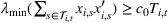
Under Assumption A, we have the following theoretical result on the regret of the CSMP algorithm. Theorem 1
Let input parameter
$c \geq 20 / l_{1}^{2}$
; the expected regret of algorithm CSMP is
$R (T) = O (\frac{d^{2} \log^{2} (d T)}{\min_{i \in [n]} q_{i}^{2}} + d \sqrt{m T} \log T) .$
15
In particular, if
$q_{i} = Θ (1 / n)$
for all
$i \in [n]$
and we hide the logarithmic terms, then when
$T ≫ n$
, the expected regret is at most
$\tilde{O} (d \sqrt{m T})$
.

Here, we briefly discuss the very high‐level ideas of proving Theorem 1, with the technical details deferred to the Supporting Information. One key step of proving the main part of the regret
$\tilde{O} (d \sqrt{m T})$
, as opposed to the typical regret
$\tilde{O} (d \sqrt{n T})$
for single‐product pricing without clustering, is that we are able to identify each neighborhood correctly. This is achieved by our technique of price perturbation, which guarantees that our estimated parameter
${\hat{θ}}_{i, t}$
converges to the true
$θ_{i}$
in a sufficiently fast rate. As a result, when
$t \geq \bar{t} = Θ (d^{2} \log^{2} (d T) / (\min_{i \in [n]} q_{i}^{2}))$
(this is why we have regret
$O (d^{2} \log^{2} (d T) / (\min_{i \in [n]} q_{i}^{2}))$
, which is incurred before
$\bar{t}$
), all neighborhoods are identified correctly with high probability. Conditioned on this, our problem is basically reduced to the pricing of m “products,” which gives us the regret
$\tilde{O} (d \sqrt{m T})$
.

Although the key ideas are quite simple, the proofs are technical and involved, which differ from the existing literature. For instance, compared with the bandit with clustering literature (see, e.g., Cesa‐Bianchi et al., 2013; Gentile et al., 2014, 2017; Nguyen & Lauw, 2014), our action set (prices) is continuous instead of finite and we have to exploit unique structure of revenue function (e.g., Assumption A) by using price perturbation techniques. Moreover, we do not assume stochasticity of context
$x_{i, t}$
—for example, contexts are i.i.d., which is also assumed in contextual pricing literature such as Ban and Keskin (2021), Chen, Owen, et al. (2022), Nambiar et al. (2019), Qiang and Bayati (2016) besides the bandit literature mentioned earlier—but only a weaker variation assumption (see Assumption A‐3). This relaxation requires us to use a different matrix analysis technique instead of directly applying matrix concentration inequalities (see Lemma EC.3 in the Supporting Information).

We have a number of remarks about the CSMP algorithm and the result on regret, following in order. Remark 4 Comparison with single‐product pricing

Our pricing policy achieves the regret

\tilde{O} (d \sqrt{m T})

. A question arises as to how it compares with the baseline single‐product pricing algorithm that treats each product separately. Ban and Keskin (2021) consider a single‐product pricing problem with demand covariates. According to Theorem 2 in Ban and Keskin (2021), their algorithm, when applied to each product i in our setting separately, achieves the regret

\tilde{O} (d \sqrt{T_{i, T}})

. Therefore, adding together all products

i \in [n]

, the upper bound of the total regret is

\tilde{O} (d \sqrt{n T})

. When the number of clusters m is much smaller than n, the regret

\tilde{O} (d \sqrt{m T})

of CSMP significantly improves the total regret obtained by treating each product separately.

Remark 5 Lower bound of regret

To obtain a lower bound for the regret of our problem, we consider a special case of our model in which the decision maker knows the underlying true clusters

N_{j}

. Since this is a special case of our problem (which is equivalent to single‐product pricing for each cluster

N_{j}

), the regret lower bound of this problem applies to ours as well. Theorem 1 in Ban and Keskin (2021) shows that the regret lower bound for each cluster j has to be at least

Ω (d \sqrt{{\tilde{T}}_{j, t}})

. In the case that

{\tilde{q}}_{j} = 1 / m

for all

j \in [m]

, it can be derived that the regret lower bound for all clusters has to be at least

Ω (d \sqrt{m T})

. This implies that the regret of the proposed CSMP policy is optimal up to a logarithmic factor.

Remark 6 Improving the regret for large n

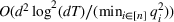
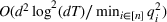
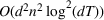
When n is large, the first term in our regret bound

O (d^{2} \log^{2} (d T) / \min_{i \in [n]} q_{i}^{2})

will also become large. For instance, if

q_{i} = O (1 / n)

for all

i \in [n]

, then this term becomes

O (d^{2} n^{2} \log^{2} (d T))

. One way to improve the regret, although it requires prior knowledge of γ, is to conduct more price exploration during the early stages. Specifically, if the confidence bound

B_{i, t - 1}

of product i is larger than

γ / 4

, in Step 4, we let the price perturbation

Δ_{i, t}

\pm Δ_{0}

to introduce sufficient price variation (otherwise let

Δ_{t}

be the same as in the original algorithm CSMP). Following a similar argument as in Lemma EC.3 in the Supporting Information, it roughly takes

O (d \log (d T) / \min_{i \in [n]} q_{i})

time periods before all

B_{i, t - 1} < γ / 4

, so the same proof used in Theorem 1 applies. Therefore, when

q_{i} = O (1 / n)

for all

i \in [n]

, the final regret upper bound is

O (d n \log (d T) + d \log T \sqrt{m T})

Remark 7 Relaxing the cluster assumption

Our theoretical development assumes that products within the same cluster have exactly the same parameters

θ_{i}

. This assumption can be relaxed as follows. Without loss of generality, let us assume all products have different

θ_{i}

. Define two products

i_{1}, i_{2}

as in the same cluster if they satisfy

| | θ_{i_{1}} - θ_{i_{2}} {| |}_{2} \leq γ_{0}

for some positive constant γ₀ with

γ_{0} < γ / 3

. Our policy in Algorithm 1 can adapt to this case by modifying Step 2 to

\begin{matrix} {\hat{N}}_{i, t} = {i^{'} \in [n] : | | {\hat{θ}}_{i^{'}, t - 1} - {\hat{θ}}_{i, t - 1} {| |}_{2} \leq 2 B_{i^{'}, t - 1} + 2 B_{i, t - 1}} . \end{matrix}

The reason we make this modification is that when t is within certain range,

| | {\hat{θ}}_{i^{'}, t - 1} - {\hat{θ}}_{i, t - 1} {| |}_{2} > 2 B_{i^{'}, t - 1} + 2 B_{i, t - 1}

implies that, with high probability,

| | θ_{i^{'}, t - 1} - θ_{i, t - 1} {| |}_{2} > B_{i^{'}, t - 1} + B_{i, t - 1} > γ_{0}

. This shows we can correctly differentiate the products, which are not in the same cluster. As a result, under this modification, our algorithm CSMP has the following performance. If

T \leq O (1 / (\max_{i} q_{i}^{2} γ_{0}^{4}))

, the regret is at most

\tilde{O} (d \sqrt{m T} + \min {γ_{0}^{2} \sum_{j} {\tilde{q}}_{j}^{2} T^{2}, T})

. Thus when T is small, the main difference with Theorem 1 is the extra term

O (\min {γ_{0}^{2} \sum_{j} {\tilde{q}}_{j}^{2} T^{2}, T})

due to relaxation of clusters, and if γ₀ is small, we still have the overall regret better than

\tilde{O} (d \sqrt{n T})

without any clustering. On the other hand, for large T and in particular, when

T \to \infty

, we show that the regret will approach

\tilde{O} (d \sqrt{n T})

. Intuitively, this is because when the data are no longer scarce, our clustering actually identifies each product i as its own cluster, reducing to the single‐product pricing algorithm without clustering. For detailed analysis of this relaxation, we refer the interested readers to Section EC.2 in the Supporting Information.

One relevant stream of literature to this setting is the so‐called bandit with model mis‐specification, which assumes that the reward function is mis‐specified with error ε (see, e.g., Crammer & Gentile, 2013; Foster & Rakhlin, 2020; Foster et al., 2020; Ghosh et al., 2017; Lattimore et al., 2020), and they show that the part of regret related to ε has to be

Ω (ε T)

. Our method in this setting is different in that we only take advantage of the γ₀‐different parameters (γ₀ is typically very small) in the same cluster when data are scarce (i.e., T is small). As more data are gathered, the algorithm naturally converges to single‐product pricing, making our regret in the long run still being sublinear in T.

SIMULATION RESULTS WITH SYNTHETIC AND REAL DATA

This section provides the simulation experiment results for algorithm CSMP. First, we conduct a simulation study using synthetic data in Section 4.1 to illustrate the effectiveness and robustness of our algorithms against several benchmark approaches. Second, the simulation results using a real data set from Alibaba are provided in Section 4.2. Finally, we summarize all numerical experiment results in Section 4.3.

Simulation using synthetic data

In this section, we demonstrate the effectiveness of our algorithms using some synthetic data simulation. We first show the performance of CSMP against several benchmark algorithms. Then, several robustness tests are conducted for CSMP. The first test is for the case when clustering assumption is violated (i.e., parameters within the same cluster are slightly different). The second test is when the demand covariates

z_{i, t}

contain some features that change slowly in a deterministic manner. Finally, we test CSMP with a misspecified demand model.

We shall compare the performance of our algorithms with the following benchmarks:

The SMP algorithm, which treats each product independently (IND), and we refer to it as SMP‐IND.

The SMP algorithm, which treats all products as one (ONE) single cluster, and we refer to the algorithm as SMP‐ONE.

The CSMP with K‐means Clustering (CSMP‐KMeans), which uses K‐means clustering for product clustering in Step 2 of CSMP.

The first two benchmarks are natural special cases of our algorithm. Algorithm SMP‐IND skips the clustering step in our algorithm and always sets the neighborhood as

{\hat{N}}_{t} = {i_{t}}

; while SMP‐ONE keeps

{\hat{N}}_{t} = N

for all

t \in [T]

. The last benchmark is to test the effectiveness of other classical clustering approach for our setting, in which we choose K‐means clustering as an illustrative example because of its popularity.

Logistic demand with clusters

For illustration of a GLM demand, we simulate using a logistic function. We set the time horizon

T = 30, 000

, the searching probability

q_{i} = 1 / n

for all

i \in [n]

where

n = 100

, and the price range

\underset{̲}{p} = 0

and

\bar{p} = 10

. In this study, it is assumed that all

n = 100

products have

m = 10

clusters (with products randomly assigned to clusters). Within a cluster j, each entry in

α_{j}

is generated uniformly from

[- L / \sqrt{d + 2}, L / \sqrt{d + 2}]

with

L = 10

, and

β_{j}

is generated uniformly from

[- L / \sqrt{d + 2}, 0)

(to guarantee that

| | θ_{i} {| |}_{2} \leq L

). For demand covariates, each feature in

z_{i, t}

, with dimension

d = 5

, is generated independently and uniformly from

[- 1 / \sqrt{d}, 1 / \sqrt{d}]

(to guarantee that

| | z_{i, t} {| |}_{2} \leq 1

). For the parameters in the algorithms, we let

Δ_{0} = 1

; and for the confidence bound

B_{i, t} = \sqrt{c (d + 2) \log (1 + t) / λ_{\min} (V_{i, t})}

, we first let

c = 0.8

and then test other values of c for sensitivity analysis. For the benchmark CSMP‐KMeans, we need to specify the number of clusters K; since the true number of clusters m is not known a priori, we test different values of K in

{5, 10, 20, 30}

. Note that when

K = 10

, the performance of CSMP‐KMeans can be considered as an oracle since it correctly specifies the true number of product clusters.

To evaluate the performance of algorithms, we adopt both the cumulative regret in (6) and the percentage revenue loss defined by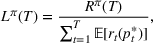

L^{π} (T) = \frac{R^{π} (T)}{\sum_{t = 1}^{T} E [r_{t} (p_{t}^{*})]},

which measures the percentage of revenue loss with respect to the optimal revenue. Obviously, the percentage revenue loss and cumulative regret are equivalent, and a better policy leads to a smaller regret and a smaller percentage revenue loss.

For each experiment, we conduct 30 independent runs and take their average as the output. We also output the standard deviation of percentage revenue loss for all policies in Table 1. It can be seen that our policy CSMP has quite small standard deviation, so we will neglect standard deviation results in other experiments.

TABLE 1

Standard deviation (%) of percentage revenue loss corresponding to different time periods for logistic demand with 10 clusters

	t = 5,000	t = 10,000	t = 15,000	t = 20,000	t = 25,000	t = 30,000
CSMP	1.83	0.97	0.70	0.57	0.47	0.40
SMP‐IND	1.32	0.88	0.92	0.81	0.78	0.73
SMP‐ONE	2.34	2.15	1.75	1.44	1.46	1.44
CSMP‐KMeans: $K = 5$	2.08	1.97	1.95	2.26	2.22	2.19
CSMP‐KMeans: $K = 10$	2.06	1.53	1.09	0.87	0.74	0.66
CSMP‐KMeans: $K = 20$	2.12	1.36	1.15	1.02	0.91	0.82
CSMP‐KMeans: $K = 30$	1.41	0.88	0.77	0.67	0.59	0.49

We recognize that a more appropriate measure for evaluating an algorithm is the regret (and percentage of loss) of expected total profit (instead of expected total revenue). We choose the latter for the following reasons. First, it is consistent with the objective of this paper, which is the choice of the existing literature. Second, it is revenue, not profit, that is being evaluated at our industry partner, Alibaba. Third, even if we wish to measure it using profit, the cost data of products are not available to us, since the true costs depend on such critical things as terms of contracts with suppliers, that are confidential information.

The results are shown in Figure 2. According to this figure, our algorithm CSMP outperforms all the benchmarks except for CSMP‐KMeans when

K = m = 10

. CSMP‐KMeans with

K = 10

has the best performance, which is not surprising because it uses the exact and correct number of clusters. However, in reality the true cluster number m is not known. We also test CSMP‐KMeans with

K = 5, 20, 30

. We find that when

K = 20

, its performance is similar to (slightly worse than) our algorithm CSMP. When

K = 5, 30

, the performance of CSMP‐KMeans becomes much worse (especially when

K = 5

). For the other two benchmarks SMP‐ONE and SMP‐IND, their performances are not satisfactory either, with SMP‐ONE has the worst performance because clustering all products together leads to significant error. Sensitivity results of CSMP with different parameters c are presented in Table 2, and it can be seen that CSMP is quite robust with different values of c.

TABLE 2

Mean and standard deviation (%) of percentage revenue loss of CSMP (logistic demand with 10 clusters) with different parameters c

	$c = 0.5$	$c = 0.6$	$c = 0.7$	$c = 0.8$	$c = 0.9$	$c = 1.0$
Mean	8.56	8.28	8.52	8.27	8.56	8.72
Standard deviation	0.73	0.51	0.73	0.40	0.66	0.35

FIGURE 2

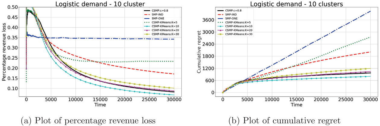
Performance of different policies for logistic demand with 10 clusters. The graph on the left‐hand side shows the percentage revenue loss of all algorithms, and the graph on the right‐hand side shows the cumulative regrets for each algorithm

Logistic demand with relaxed clusters

As we discussed in Section 3.2, strict clustering assumption might not hold and sometimes products within the same cluster are slightly different. This experiment tests the robustness of CSMP when parameters of products in the same cluster are slightly different. To this end, after we generate the

m = 10

centers of parameters (with each center represented by

θ_{j}

), for each product i in the cluster j, we let

θ_{i} = θ_{j} + Δ θ_{i}

where

Δ θ_{i}

is a random vector such that each entry is uniformly drawn from

[- L / (10 \sqrt{d + 2}), L / (10 \sqrt{d + 2})]

. All the other parameters are the same as in the case with 10 clusters. Results are summarized in Figure 3, and it can be seen that the performances of all algorithms are quite similar as in Figure 2.

FIGURE 3

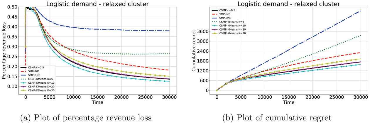
Performance of different policies for logistic demand with relaxed clusters

Logistic demand with almost static features

As we discussed after Assumption A‐3, in some applications there might be features that have little variations (nearly static). We next test the robustness of our algorithm CSMP when the feature variations are small. To this end, we assume that one feature in

z_{i, t} \in R^{d}

for each

i \in [n]

is almost static. More specifically, we let this feature be constantly

1 / \sqrt{d}

for 100 periods, then change to

- 1 / \sqrt{d}

for another 100 periods, then switch back to

1 / \sqrt{d}

after 100 periods, and this process continues. The numerical results against benchmarks are summarized in Figure 4. It can be seen that with such an almost static feature, the performances of algorithms with clustering become worse, but they still outperform the benchmark algorithms. In particular, CSMP (with parameter

c = 0.1

after a few trials of tuning) still has promising performance, showing its robustness with small feature variations of some products.

FIGURE 4

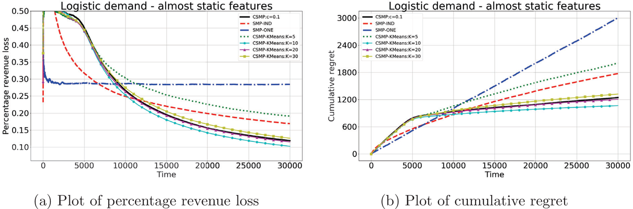
Performance of different policies for logistic demand with 10 clusters and almost static features

Logistic demand with model misspecification

In real applications, it may happen that the demand model is misspecified. In this experiment, we consider a misspecified logistic demand model. Specifically, we let the expected demand of product i be

1 / (1 + \exp (f_{i} (z_{t}, p_{t})))

, where the utility function

\begin{matrix} f_{i} (z_{t}, p_{t}) & : = & c_{i, 0} + \sum_{k = 1}^{d} c_{1, i, k} z_{t, k} + \sum_{k = 1}^{d} c_{2, i, k} z_{t, k}^{2} + \sum_{k = 1}^{d} c_{3, i, k} z_{t, k}^{3} \\ + β_{1, i} p_{t} + β_{2, i}^{2} p_{t}^{2} + β_{3, i} p_{t}^{3} \end{matrix}

is a third degree polynomial of

z_{t}, p_{t}

, where

c_{i}, β_{i}

are unknown parameters, and

z_{t, k}

represents the k‐th component of

z_{t}

. To generate this misspecified demand model, we let

c_{l, i, k} \in [- L / \sqrt{3 (d + 2)}, L / \sqrt{3 (d + 2)}]

with

l \in {1, 2, 3}, k \in [d]

c_{i, 0} \in [- L / \sqrt{d + 2}, L / \sqrt{d + 2}]

, and

β_{l, i} \in [- L / \sqrt{3 (d + 2)}, 0)

with

l \in {1, 2, 3}

, be all drawn uniformly. All the other input parameters for the problem instance are the same as in the case of logistic demand with 10 clusters.

To test the robustness of the misspecified CSMP, it is compared with CSMP, which correctly specifies the demand model. We call the benchmark the CSMP‐Oracle. The numerical results are summarized in Figure 5. As seen, when compared with the oracle, the misspecified CSMP has slightly worse performance as expected. But the overall difference in percentage revenue loss is only 3.48%, showing that our algorithm CSMP is rather robust with such a model misspecification.

FIGURE 5

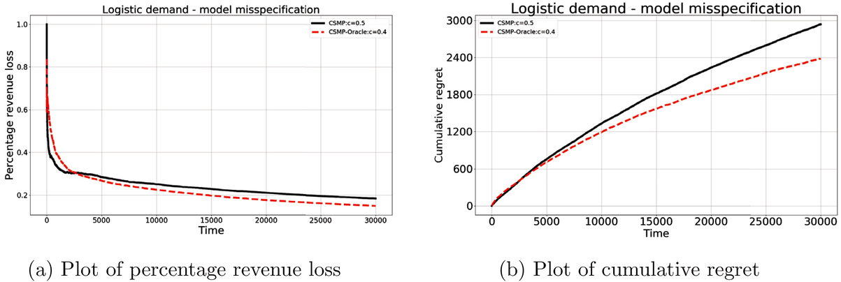
Performance of CSMP with (misspecified) logistic demand versus the oracle

Simulation using real data from Alibaba

This section presents the results of our algorithms (for illustration, we use CSMP with logistic demand) and other benchmarks using a real data set provided by Alibaba. To better simulate the real demand process, we fit the demand data to create a sophisticated ground truth model (hence our algorithm CSMP may have a model misspecification). Before presenting the results, we introduce the data set and preprocessing of the data.

The data set

To motivate our study of pricing for low‐sale products, we extract sales data from May 29, 2018, to July 28, 2018. During this period, nearly 75,000 products were offered by Tmall Supermarket. There are more than 21.6% (i.e., 16,000) products with average numbers of daily unique visits less than 10. Among all these low‐sale products, Alibaba provided us with a test data set comprising 100 products that have at least one sale during the 61‐day period, and at least two prices charged with each price offered to more than 10% of all customers. Because these selected products have relatively sufficient variation of prices and different observations of customers' purchases, demand parameters can be estimated quite accurately using the sales data in the data set. As the focus of this paper is on single‐product pricing where the demand of each product depends on its own price, this numerical study using the real data set is also conducted under this setting. In Section EC.3 in the Supporting Information, we conduct a data analysis to show that this assumption is indeed reasonable for this data set.

For the features of products, we are provided by Alibaba with five features (hence

d = 5

), that are described below:

average gross merchandise volume (GMV, i.e., product revenue) in past 30 days,

average demand in past 30 days,

average number of unique buyers (UBs, i.e., unique IP, which makes the purchase) in past 30 days,

average number of UVs in past 30 days, and

average number of independent product views (IPVs, i.e., total number of views on the product, including repetitive views from the same user) in past 30 days.

These features are selected by Alibaba's feature engineering team² (via a recursive feature elimination approach from a raw set of features). Note that these features are not exogenous, since features in the future can be affected by current pricing decision. Such endogenous features are often used in the demand forecasting literature. For instance, a time‐series model uses past demand to predict future demand (see, e.g., Brown, 1959); an artificial neural network (ANN) model uses historical demand data of composite products as features for demand prediction (Chang et al., 2005). In the pricing literature, some endogenous features have also been used. For example, in Ban and Keskin (2021) and Bastani et al. (2022), their model features include auto loan data, for example, competitors' rate, that are affected by the rate offered by the decision maker (the auto loan company). Incorporating the impact of pricing decisions on features leads to challenging dynamic programming problem with partial information. Hence, features are considered as given and we only optimize for current period (i.e., ignoring the long‐run effect of the current pricing decision).

To understand the data and features better, we provide a summary statistics on the data and feature. First, we calculated the number of prices charged during the time horizon, average demand per day, average UV per day, and average IPV per day, for each one of the selected 100 products. Table 3 summarizes the mean and standard deviation of each of the data. Then, to understand the variation of features, we calculated the standard deviation of each of the five features of every product. In Table 4 we summarize the mean and standard deviation of feature variations of all products.

TABLE 3

Summary statistics of average data of the 100 products

	Number of prices	Demand	UV	IPV
Mean	7.13	0.71	6.88	10.13
Standard deviation	5.16	0.72	2.04	3.38

TABLE 4

Summary statistics of feature variation of the 100 products

	Feature GMV	Feature demand	Feature UB	Feature UV	Feature IPV
Mean	12.93	0.34	0.49	5.04	7.73
Standard deviation	17.97	0.60	0.89	9.21	13.95

To run simulation using the real data set, we first create a ground truth model for the demand. We consider two ground truth models in this simulation study. The first one is the commonly used logistic demand function (hence no model misspecification for our algorithm CSMP), and the second is a random forest model (as used in simulation study of Nambiar et al., 2019, hence there is model misspecification for CSMP). We use the demand data of each product to fit these two demand models, and then apply them to simulate the demand process. To test the accuracy of these two demand models, we calculated the average receiver operating characteristic area under the curve (ROC‐AUC) score (among the selected products) of the logistic and random forest model, respectively. The results show that the ROC‐AUC score of the random forest model is 11.7% higher than that of the logistic model (thus the random forest model fits the reality better).

We want to generate customer's arrival at each time t, that is, the product

i_{t}

a customer chooses to search. Since the data set contains the daily number of UVs for each product i, the arrival process

i_{t}

is simulated by randomly permuting the UVs of each product on each day. For instance, if on day 1, product 1 and product 2 have 2 and 3 UVs respectively, then

i_{t}

for

t = 1, …, 5

can be 1,2,2,1,2, which is a random permutation of the UVs for products 1 and 2.

Numerical results for the algorithms

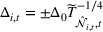
We first provide the specifications of the parameters in the CSMP algorithm in Algorithm 1.

The confidence bound

B_{i, t}

\sqrt{c (d + 2) \log (1 + t) / λ_{\min} (V_{i, t})}

, where

c = 0.01

for logistic demand and

c = 0.05

for random forest demand (selected by a few trials of different values).

The price lower bound of each product is 50% lower than its lowest price during the 61‐day period, and the price upper bound is 50% higher than its highest price during this period of time.

The basic price perturbation parameter Δ₀ of each product is set as the length of price range divided by 4, that is,

Δ_{0} = (\bar{p} - \underset{̲}{p}) / 4

For benchmark algorithms, they are the same as those in the previous subsection, with CSMP‐KMeans have

K \in {5, 10, 20, 30}

. In addition, we test another benchmark proposed in Keskin and Zeevi (2016). More specifically, this benchmark assumes a simple linear demand model as

E [d_{i, t}] = α_{i, t} + β_{i, t}^{'} p_{i, t}

with changing parameters (CPs)

α_{i, t}, β_{i, t}

but without demand covariates. Since this single‐product pricing algorithm can be considered as a modified version of SMP, we call it SMP with CPs, or SMP‐CP for short. In particular, among the algorithms proposed in Keskin and Zeevi (2016), we choose the “Moving Window Policy” as it has the best empirical performance and choose the input parameter

κ = 0.5

as in the numerical experiments in Section 6.3 in Keskin and Zeevi (2016). We plot the results of cumulative revenue at different dates in Figure 6.

FIGURE 6

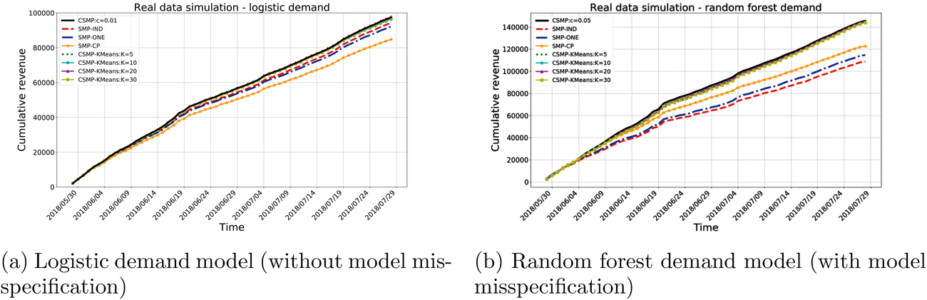
Plot of cumulative revenue over different dates for two demand models

It can be seen that all the methods using clustering have better performance, and their performances are comparable. It is interesting to note that for clustering using K‐means method, their performances with different value of K are actually quite close. Finally, it is observed that the advantage of using clustering with random forest model (i.e., misspecified model) is more than that with logistic model.

Summary of numerical experiments

In this section we first present the simulation results using synthetic data under various scenarios to test the effectiveness and robustness of our algorithms, then we present the simulation results with real data from Alibaba using a more sophisticated ground truth demand model (for a more realistic simulation and robustness test under model misspecification). The main findings from the numerical study are summarized as follows.

In all the numerical results, pricing with clustering (either using our method in CSMP or classical K‐means clustering with appropriate choice of K) outperforms the benchmarks of applying single‐product pricing algorithm on each product or naively putting all products into a single cluster.

Dynamic pricing with K‐means clustering method sometimes works as effectively as (and at times even better than) our algorithm CSMP. But its performance depends on the choice of the number of clusters K, which is unknown to the decision maker.

The CSMP algorithm is quite robust under different scenarios: slightly different demand parameters within the same cluster, near static or slowly changing features, and misspecified ground truth demand model.

CONCLUSION

With the rapid development of e‐commerce, data‐driven dynamic pricing is becoming increasingly important due to the dynamic market environment and easy access to online sales data. While there is abundant literature on dynamic pricing of normal products, the pricing of products with low sales received little attention. The data from Alibaba Group show that the number of such low‐sale products is large, and that even though the demand for each low‐sale product is small, the total revenue for all the low‐sale products is quite significant. In this paper, we present data clustering and dynamic pricing algorithms to address this challenging problem. We believe that this paper is the first to integrate online clustering learning in dynamic pricing of low‐sale products.

A learning algorithm is proposed in this paper, which learns the demand and decides product clustering simultaneously on the fly. We have established the regret bound for this under mild technical conditions. Moreover, we test our algorithms on a real data set from Alibaba Group by simulating the demand function. Numerical results show that our algorithm outperforms the benchmarks, where one either considers all products separately, or treats all products as a single cluster.

There are several possible future research directions. The first one is an in‐depth study of the method for product clustering (e.g., Gentile et al., 2014; Nguyen & Lauw, 2014). Second, to highlight the benefit of clustering techniques for low‐sale products, in this paper we study a dynamic pricing problem with sufficient inventory. One extension is to apply the clustering method for the revenue management problem with inventory constraint. Third, we believe that it will be interesting to include substitutability/complementarity of products and even assortment decisions.

Footnotes

ACKNOWLEDGMENTS

We thank the department editor, senior editor, and anonymous referees for their detailed and constructive comments that have helped to considerably improve the exposition of this paper.

1

A terminology used within Alibaba to represent a unique user login identification.

2

We requested to include some other features, such as number/score of customer ratings and competitor's price on similar product, but were unable to obtain such data due to technical reasons.

References

Abbasi‐Yadkori

Pál

Szepesvári

(2011). Improved algorithms for linear stochastic bandits. Advances in Neural Information Processing Systems, 2312–2320.

Araman

V. F.

Caldentey

(2009). Dynamic pricing for nonperishable products with demand learning. Operations Research, 57(5), 1169–1188.

Arthur

Vassilvitskii

(2007). k‐means++: The advantages of careful seeding. In Proceedings of the eighteenth annual ACM‐SIAM symposium on discrete algorithms (pp. 1027–1035).

Baardman

Levin

Perakis

Singhvi

(2018). Leveraging comparables for new product sales forecasting. Production and Operations Management, 27(12), 2340–2343.

Ban

G.‐Y.

Gallien

Mersereau

A. J.

(2018). Dynamic procurement of new products with covariate information: The residual tree method. Manufacturing & Service Operations Management, 21(4), 798–815.

Ban

G.‐Y.

Keskin

N. B.

(2021). Personalized dynamic pricing with machine learning: High‐dimensional features and heterogeneous elasticity. Management Science, 67(9), 5549–5568.

Bastani

Simchi‐Levi

Zhu

(2022). Meta dynamic pricing: Transfer learning across experiments. Management Science, 68(3), 1865–1881.

Bernstein

Modaresi

Sauré

(2018). A dynamic clustering approach to data‐driven assortment personalization. Management Science, 65(5), 2095–2115.

Bertsimas

Perakis

(2006). Dynamic pricing: A learning approach. In Lawphongpanich, Siriphong, Hearn, Donald W., & Smith, Michael J. (Eds), Mathematical and computational models for congestion charging (pp. 45–79). Springer.

10.

Besbes

Gur

Zeevi

(2015). Non‐stationary stochastic optimization. Operations Research, 63(5), 1227–1244.

11.

Besbes

Zeevi

(2009). Dynamic pricing without knowing the demand function: Risk bounds and near‐optimal algorithms. Operations Research, 57(6), 1407–1420.

12.

Besbes

Zeevi

(2015). On the (surprising) sufficiency of linear models for dynamic pricing with demand learning. Management Science, 61(4), 723–739.

13.

Bitran

Caldentey

(2003). An overview of pricing models for revenue management. Manufacturing & Service Operations Management, 5(3), 203–229.

14.

Broder

Rusmevichientong

(2012). Dynamic pricing under a general parametric choice model. Operations Research, 60(4), 965–980.

15.

Brown

R. G.

(1959). Statistical forecasting for inventory control. McGraw/Hill.

16.

Bubeck

Cesa‐Bianchi

(2012). Regret analysis of stochastic and nonstochastic multi‐armed bandit problems. Foundations and Trends® in Machine Learning, 5(1), 1–122.

17.

Carvalho

A. X.

Puterman

M. L.

(2005). Learning and pricing in an internet environment with binomial demands. Journal of Revenue and Pricing Management, 3(4), 320–336.

18.

Cesa‐Bianchi

Gentile

Zappella

(2013). A gang of bandits. Advances in Neural Information Processing Systems, 26, 737–745.

19.

Chang

P.‐C.

Wang

Y.‐W.

Tsai

C.‐Y.

(2005). Evolving neural network for printed circuit board sales forecasting. Expert Systems with Applications, 29(1), 83–92.

20.

Chen

Gallego

(2021). Nonparametric pricing analytics with customer covariates. Operations Research, 69(3), 974–984.

21.

Chen

Jasin

Duenyas

(2015). Real‐time dynamic pricing with minimal and flexible price adjustment. Management Science, 62(8), 2437–2455.

22.

Chen

Gao

Wang

(2022). Bayesian dynamic learning and pricing with strategic customers. Production and Operations Management, 00, 1–18.

23.

Chen

Miao

Wang

(2021). Differential privacy in personalized pricing with nonparametric demand models. Available at SSRN 3919807.

24.

Chen

Owen

Pixton

Simchi‐Levi

(2022). A statistical learning approach to personalization in revenue management. Management Science, 68(3), 1923–1937.

25.

Chen

Simchi‐Levi

Wang

(2022). Privacy‐preserving dynamic personalized pricing with demand learning. Management Science .

26.

Chen

Wang

(2022). Robust dynamic pricing with demand learning in the presence of outlier customers. Operations Research .

27.

Chen

Shi

(2019). Network revenue management with online inverse batch gradient descent method. Available at SSRN 3331939.

28.

Cheung

W. C.

Simchi‐Levi

Wang

(2017). Dynamic pricing and demand learning with limited price experimentation. Operations Research, 65(6), 1722–1731.

29.

Cohen

M. C.

Lobel

Perakis

(2018). Dynamic pricing through data sampling. Production and Operations Management, 27(6), 1074–1088.

30.

Crammer

Gentile

(2013). Multiclass classification with bandit feedback using adaptive regularization. Machine Learning, 90(3), 347–383.

31.

Cross

R. G.

(1995). An introduction to revenue management. In Handbook of airline economics (pp. 443‐458). McGraw‐Hill, Incorporated.

32.

denBoer

A. V.

(2015). Dynamic pricing and learning: Historical origins, current research, and new directions. Surveys in Operations Research and Management Science, 20(1), 1–18.

33.

denBoer

A. V.

Zwart

(2013). Simultaneously learning and optimizing using controlled variance pricing. Management Science, 60(3), 770–783.

34.

Dunn

J. C.

(1973). A fuzzy relative of the isodata process and its use in detecting compact well‐separated clusters. Journal of Cybernetics, 3(3), 32–57.

35.

Elmaghraby

Keskinocak

(2003). Dynamic pricing in the presence of inventory considerations: Research overview, current practices, and future directions. Management Science, 49(10), 1287–1309.

36.

Farias

V. F.

Van Roy

(2010). Dynamic pricing with a prior on market response. Operations Research, 58(1), 16–29.

37.

Ferreira

K. J.

Lee

B. H. A.

Simchi‐Levi

(2015). Analytics for an online retailer: Demand forecasting and price optimization. Manufacturing & Service Operations Management, 18(1), 69–88.

38.

Ferreira

K. J.

Simchi‐Levi

Wang

(2018). Online network revenue management using thompson sampling. Operations Research, 66(6), 1586–1602.

39.

Foster

Rakhlin

(2020). Beyond UCB: Optimal and efficient contextual bandits with regression oracles. In III, Hal Daumé & Singh, Aarti (Eds.), International conference on machine learning (pp. 3199–3210). PMLR.

40.

Foster

D. J.

Gentile

Mohri

Zimmert

(2020). Adapting to misspecification in contextual bandits. Advances in Neural Information Processing Systems, 33, 11478–11489.

41.

Gallego

Van Ryzin

(1994). Optimal dynamic pricing of inventories with stochastic demand over finite horizons. Management Science, 40(8), 999–1020.

42.

Gallego

Van Ryzin

(1997). A multiproduct dynamic pricing problem and its applications to network yield management. Operations Research, 45(1), 24–41.

43.

Gentile

Kar

Karatzoglou

Zappella

Etrue

(2017). On context‐dependent clustering of bandits. In Precup, Doina & Teh, Yee Whye (Eds.), International conference on machine learning (pp. 1253–1262). PMLR.

44.

Gentile

Zappella

(2014). Online clustering of bandits. In Xing, Eric P. & Jebara, Tony (Eds.), International conference on machine learning (pp. 757–765).

45.

Ghosh

Chowdhury

S. R.

Gopalan

(2017). Misspecified linear bandits. In thirty‐first AAAI conference on artificial intelligence .

46.

Harrison

J. M.

Keskin

N. B.

Zeevi

(2012). Bayesian dynamic pricing policies: Learning and earning under a binary prior distribution. Management Science, 58(3), 570–586.

47.

Acimovic

Erize

Thomas

D. J.

Van Mieghem

J. A.

(2018). Forecasting new product life cycle curves: Practical approach and empirical analysis: Finalist–2017 M&SOM practice‐based research competition. Manufacturing & Service Operations Management, 21(1), 66–85.

48.

Jagabathula

Subramanian

Venkataraman

(2018). A model‐based embedding technique for segmenting customers. Operations Research, 66(5), 1247–1267.

49.

Javanmard

Nazerzadeh

(2019). Dynamic pricing in high‐dimensions. Journal of Machine Learning Research, 20(9), 1–49.

50.

Keskin

N. B.

Sunar

(2020). Data‐driven clustering and feature‐based retail electricity pricing with smart meters. Available at SSRN 3686518.

51.

Keskin

N. B.

Zeevi

(2014). Dynamic pricing with an unknown demand model: Asymptotically optimal semi‐myopic policies. Operations Research, 62(5), 1142–1167.

52.

Keskin

N. B.

Zeevi

(2016). Chasing demand: Learning and earning in a changing environment. Mathematics of Operations Research, 42(2), 277–307.

53.

Kumar

Mookerjee

Shubham

(2018). Research in operations management and information systems interface. Production and Operations Management, 27(11), 1893–1905.

54.

Lattimore

Szepesvari

Weisz

(2020). Learning with good feature representations in bandits and in RL with a generative model. In III, Hal Daumé & Singh, Aarti (Eds.), International conference on machine learning (pp. 5662–5670). PMLR.

55.

Lei

Y. M.

Jasin

Sinha

(2014). Near‐optimal bisection search for nonparametric dynamic pricing with inventory constraint. Available at SSRN 2509425.

56.

Lobel

Leme

R. P.

Vladu

(2018). Multidimensional binary search for contextual decision‐making. Operations Research, 66(5), 1346–1361.

57.

MacQueen

, et al. (1967). Some methods for classification and analysis of multivariate observations. In Lucien M. Le Cam, & Jerzy Neyman (Eds.), Proceedings of the fifth Berkeley symposium on mathematical statistics and probability (Vol. 1, pp. 281–297).

58.

McCullagh

Nelder

J. A.

(1989). Generalized linear models, vol. 37. CRC press.

59.

Murtagh

(1983). A survey of recent advances in hierarchical clustering algorithms. The Computer Journal, 26(4), 354–359.

60.

Nambiar

Simchi‐Levi

Wang

(2019). Dynamic learning and pricing with model misspecification. Management Science, 65(11), 4980–5000.

61.

Nguyen

T. T.

Lauw

H. W.

(2014). Dynamic clustering of contextual multi‐armed bandits. In Proceedings of the 23rd ACM international conference on conference on information and knowledge management (pp. 1959–1962). ACM.

62.

Qiang

Bayati

(2016). Dynamic pricing with demand covariates. Available at SSRN 2765257.

63.

Saxena

Prasad

Gupta

Bharill

Patel

O. P.

Tiwari

M. J.

Ding

Lin

C.‐T.

(2017). A review of clustering techniques and developments. Neurocomputing, 267, 664–681.

64.

Shi

Malik

(2000). Normalized cuts and image segmentation. IEEE Transactions on Pattern Analysis and Machine Intelligence, 22(8), 888–905.

65.

Smith

B. C.

Leimkuhler

J. F.

Darrow

R. M.

(1992). Yield management at American airlines. Interfaces, 22(1), 8–31.

66.

Chen

(2015). A method for discovering clusters of e‐commerce interest patterns using click‐stream data. Electronic Commerce Research and Applications, 14(1), 1–13.

67.

Tropp

J. A.

(2011). User‐friendly tail bounds for matrix martingales . ACM Report 2011–01, California Inst. of Tech. Pasadena, CA.

68.

Van Kampen

T. J.

Akkerman

Pieter van Donk

(2012). Sku classification: A literature review and conceptual framework. International Journal of Operations & Production Management, 32(7), 850–876.

69.

Von Luxburg

(2007). A tutorial on spectral clustering. Statistics and Computing, 17(4), 395–416.

70.

Walton

Zhang

(2020). Perturbed pricing. arXiv preprint arXiv:2010.12300.

71.

Wang

Chen

Chang

(2021). Uncertainty quantification for demand prediction in contextual dynamic pricing. Production and Operations Management, 30(6), 1703–1717.

72.

Wang

Deng

(2014). Close the gaps: A learning‐while‐doing algorithm for single‐product revenue management problems. Operations Research, 62(2), 318–331.

Context‐based dynamic pricing with online clustering

Abstract

Keywords

INTRODUCTION

Contributions of this paper

Literature review

Related literature in dynamic pricing

Related literature in clustering for pricing

Related literature in other operations management problems

Related literature in multiarm bandit problem

Related literature in clustering

Organization of the paper

PROBLEM FORMULATION

The firm's optimization problem and regret

Cluster of products

PRICING POLICY AND MAIN RESULTS

Description of the pricing policy

Parameter estimation of GLM

Determining the neighborhood of each product

Setting the price of each product

Theoretical performance of the CSMP algorithm

Remark 5 Lower bound of regret

Remark 6 Improving the regret for large n

Remark 7 Relaxing the cluster assumption

SIMULATION RESULTS WITH SYNTHETIC AND REAL DATA

Simulation using synthetic data

Logistic demand with clusters

Logistic demand with relaxed clusters

Logistic demand with almost static features

Logistic demand with model misspecification

Simulation using real data from Alibaba

The data set

Numerical results for the algorithms

Summary of numerical experiments

CONCLUSION

Footnotes

ACKNOWLEDGMENTS

1

2

References

Require: c, the confidence bound parameter; Δ₀, price perturbation parameter;
1:	Step 0. Initialization. Initialize $T_{i, 0} = \emptyset$ and $V_{i, 0} = I$ for all $i \in [n]$ . Let $t = 1$ and go to Step 1.
2:	for $t = 1, 2, …, T$ do
3:	Step 1. Individual Parametric Estimation. Compute the MLE using individual data ${\hat{θ}}_{i, t - 1} = {arg min}_{θ \in Θ} \sum_{s \in T_{i, t - 1}} l_{s} (θ)$ for all $i \in [n]$ . Go to Step 2.
4:	Step 2. Neighborhood Construction. Compute the neighborhood of each product i as ${\hat{N}}_{i, t} = {i^{'} \in [n] : \| \| {\hat{θ}}_{i^{'}, t - 1} - {\hat{θ}}_{i, t - 1} {\| \|}_{2} \leq B_{i^{'}, t - 1} + B_{i, t - 1}}$ where $B_{i, t - 1}$ is defined in (12) for each $i \in [n]$ . Go to Step 3.
5:	Step 3. Clustered Parametric Estimation. Compute the MLE using clustered data ${({\tilde{α}}_{{\hat{N}}_{i, t}, t - 1}^{'}, {\tilde{β}}_{{\hat{N}}_{i, t}, t - 1})}^{'} = {\tilde{θ}}_{{\hat{N}}_{i, t}, t - 1} = {arg min}_{θ \in Θ} \sum_{s \in {\tilde{T}}_{{\hat{N}}_{i, t}, t - 1}} l_{s} (θ)$ for each $i \in [n]$ . Go to Step 4.
6:	Step 4. Pricing. Compute price for each $i \in [n]$ as $p_{i, t}^{'} = {arg max}_{p \in [\underset{̲}{p}, \bar{p}]} μ (α_{{\hat{N}}_{i, t}, t - 1}^{'} x_{i, t} + β_{{\hat{N}}_{i, t}, t - 1} p) p,$ then project to ${\tilde{p}}_{i, t} = {Proj}_{[\underset{̲}{p} + \| Δ_{i, t} \|, \bar{p} - \| Δ_{i, t} \|]} (p_{i, t}^{'})$ and offer to the customer price $p_{i, t} = {\tilde{p}}_{i, t} + Δ_{i, t}$ where $Δ_{i, t} = \pm Δ_{0} {\tilde{T}}_{{\hat{N}}_{i, t}, t}^{- 1 / 4}$ which takes two signs with equal probability.
7:	Then, customer t arrives, searches for product $i_{t}$ , and makes purchasing decision $d_{i_{t}, t} (p_{i_{t}, t}; z_{i_{t}, t})$ . Update $T_{i_{t}, t} = T_{i_{t}, t - 1} \cup {t}$ and $V_{i_{t}, t} = V_{i_{t}, t - 1} + u_{t} u_{t}^{'}$ .
8:	end for