We consider a dynamic pricing and learning problem where a seller prices multiple products and learns from sales data about unknown demand. We study the parametric demand model in a Bayesian setting. To avoid the classical problem of incomplete learning, we propose dithering policies under which prices are probabilistically selected in a neighborhood surrounding the myopic optimal price. By analyzing the effect of dithering in facilitating learning, we establish regret upper bounds for three typical settings of demand model. We show that the dithering policy achieves an upper bound of order when the parameter set is finite. It can be modified to achieve a constant regret bound under an additional assumption. We also prove an upper bound of order when the parameter set is compact and convex. Each bound matches (up to a logarithmic factor) the existing lower bound of any pricing policy. In this way, we show that dithering policies achieve asymptotically optimal performance in three different parameter settings, which demonstrates dithering as a unified approach to strike the balance between exploration and exploitation.
We study a dynamic pricing and learning problem with unknown demand and multiple products. A seller sequentially chooses prices to maximize the revenue and learns, via Bayesian updating, about the underlying demand model from sales data. There is a trade‐off between the exploration of the optimal price and exploitation of immediate profits. This paper focuses on presenting a simple approach to strike the balance between exploration and exploitation and construct asymptotically optimal pricing policies.
We consider a customized pricing problem where the seller can set prices for each customer and observe the sales (Phillips, 2005). The selling probabilities of products are captured by a demand model that does not change over time. If the demand model is known, the seller would always choose the optimal price to maximize the total expected revenue. Unfortunately, we do not have full information about demand in common practice, which requires the seller to learn from sales data. We adopt a Bayesian approach for learning. Specifically, we consider a parameterized demand model where the parameter for each product is unknown but from a given compact set (which can be finite or uncountable). The seller starts with a prior belief on each parameter, which is evaluated through prior information such as past experience and market surveys. After setting prices for a customer and observing the sales, the seller updates the belief via Bayes' rule. Based on the parameter estimates, the posterior belief under a good pricing policy should converge to the underlying parameter, and ideally, at a fast rate.
Following the existing literature in dynamic pricing with incomplete information, we aim to identify asymptotically optimal policies under the objective of regret. To achieve this, one needs to distinguish the underlying demand model from others. For any pair of possible price–demand curves of a product, the price that corresponds to their intersection gives no information to tell them apart, and therefore it does not help the seller with learning. However, a seller seeking revenue maximization may keep choosing these prices and end up not knowing the true demand model. This phenomenon is the problem of incomplete learning, as first illustrated by Rothschild (1974). Even in a basic problem with a single product and two demand models, there can be multiple intersection points between the demand models, and any one of them may lead to incomplete learning. If we incorporate multiple products, where the demand models depend on a price vector rather than a single price, the intersection between two demand models is a collection of hypersurfaces in the high‐dimensional space. Parametric demand models, where the parameter set can be finite or even uncountable, can lead to a larger number of intersection points, which further complicates the problem.
To address the problem of incomplete learning, a good pricing policy must incorporate learning and strike a balance between exploration and exploitation. The trade‐off has been well studied in the classic multi‐armed bandit (MAB) literature, and powerful methods have been developed to handle the trade‐off. For example, upper confidence bound (UCB) algorithms choose actions (e.g., prices) that have been played for a relatively small number of times (Auer et al., 2002), the ε‐greedy algorithm explores by randomly choosing actions once in a while (Auer et al., 2002), and Thompson Sampling (TS) selects actions based on samples from the posterior (Agrawal & Goyal, 2012). These algorithms have been proven to be asymptotically optimal in the standard MAB setting. Different from the MAB problem, the dynamic pricing and learning problem has an infinite number of actions in general, and actions are connected by the underlying demand model. In this stream of literature, Harrison et al. (2012) show that the widely used myopic policy that chooses the best‐guess price can result in incomplete learning. A common approach to circumvent this difficulty is to introduce constraints to the myopic decisions to guarantee sufficient price exploration (e.g., den Boer, 2014; den Boer & Zwart, 2014; Harrison et al., 2012). Another approach is to identify prices for exploration and choose them occasionally to provide sufficient information (e.g., Broder & Rusmevichientong, 2012; Cheung et al., 2017). Both approaches have been shown to achieve reasonably good performance in different settings.
The goal of our paper is to propose an alternative approach to address incomplete learning. The approach is based on dithering, which we call Bayesian dithering in our Bayesian context. The basic idea behind Bayesian dithering is simple. By adding a random perturbation to a solution given by a deterministic pricing policy, we provide sufficient price variations to activate demand learning and avoid getting stuck in a single price vector. More specifically, dithering enables us to gather information from a set of candidate price vectors rather than a single one whenever making a pricing decision. The random perturbation in dithering offers a high chance to avoid the prices associated with incomplete learning. Insufficient dithering restricts the amount of exploration, while excessive dithering incurs a considerable loss in the immediate revenue. The balance captures the tension between learning and earning.
Dithering can serve as a unified way to balance the exploration–exploitation trade‐off in various settings. To illustrate this point, we show that dithering policies achieve asymptotically optimal performance in three typical settings of demand models studied in the literature: a finite number of demand models (Cheung et al., 2017), a “learnable” special case with a finite number of demand models (Harrison et al., 2012), and the parametric demand model with a compact and convex parameter set (Broder & Rusmevichientong, 2012). Although these papers consider problems with a single product, our results work for multiple products. We call the multiproduct extensions of the aforementioned problems the finite parameter case, the discriminative case, and the continuous parameter case, respectively.
Following the literature, we measure the performance of a policy by regret, that is, the cumulative expected revenue loss compared to a clairvoyant who knows the underlying demand model over a selling horizon of T periods. In this paper, we apply the dithering approach to the myopic Bayesian policy (MBP). In each period, the price is chosen by taking the best‐guess price and then adding a uniformly distributed perturbation to it. The dithering level—namely, the amount of the perturbation—decreases over time. For each of the three problems above, we establish a regret upper bound for the dithering policy, which matches (up to a logarithmic factor) the existing lower bound of any pricing policy, as shown in Table 1. Our analysis bounds the regret above with the rate of learning and the cost of dithering, and we control the dithering levels to obtain the best regret bounds. The rate of learning captures how the posterior distribution gradually becomes concentrated on the underlying parameter as the seller learns through dithering. A careful analysis of the Bayesian updating process is required to establish a bound on the rate of learning, which distinguishes our work from papers that take a frequentist approach for learning. Specifically, we prove a structural property that shows the role of dithering in activating demand learning, which is further used to analyze the posterior distribution. For the finite parameter case and the discriminative case, there are a finite number of potential parameters. Compared to the underlying parameter, any other parameter becomes less “likely” as more data are gathered for learning. The analysis of each parameter can be gathered together to provide an upper bound on the rate of learning. However, this method cannot be applied directly to the continuous parameter case since there is an uncountable number of potential parameters. We then introduce a suitable discretization of the parameter set and analyze each instance instead.
Regret upper bounds for Bayesian dithering and existing lower bounds
Upper bound for Bayesian‐dithering
Existing lower bound
The finite parameter case
The discriminative case
O(1)
Ω(1)
The continuous parameter case
Note: The upper bounds we show in this paper for dithering policies are presented and compared to the lower bounds in the existing literature. The lower bounds for the finite and continuous parameter cases are established in Cheung et al. (2017) and Broder and Rusmevichientong (2012), respectively. When demand is unknown, any pricing policy must incur some revenue loss compared to the clairvoyant's policy, which yields the lower bound Ω(1) for the discriminative case.
Other relevant literature
In this paper, we present dithering as a unified approach to strike the balance between exploration and exploitation in the context of dynamic pricing. In particular, we show that dithering policies achieve asymptotically optimal performance in three typical settings studied in the literature. We now provide a review on relevant papers for each class of problems. For a comprehensive survey about the dynamic pricing and learning problem, we refer to the paper by den Boer (2015).
The Finite Parameter Case. Cheung et al. (2017) consider learning from a given family of demand models for a single product. Since the number of demand models is finite, one can view this problem as parameter learning from a finite set, which is the finite parameter case we consider. They establish a lower bound of order
on the worst‐case regret of any pricing policy. They impose a fixed maximum number of price changes and design an algorithm that achieves a matching upper bound on regret. Their algorithm avoids incomplete learning by choosing prices that give the most information for learning. It operates in phases with predetermined lengths. A fixed price is chosen in each phase to reduce the number of price changes. The lengths of the phases are of order
, so the algorithm requires knowing T in advance. In contrast, we do not consider the constraint on price changes, and the dithering policy can operate without knowing T. They also consider a special case in which all demand models have an optimal price that gives different values by any pair of demand models, which is the discriminative case we consider. A similar phase‐based algorithm is given, but the fixed price in each phase is chosen from a finite set that contains all “discriminative” optimal prices. When the constraint on price changes is removed, they show a constant regret bound for the algorithm, which is the best possible. We note that their algorithms rely on the finite number of demand models and cannot be applied directly when the number of parameters is uncountable.
The Discriminative Case. Harrison et al. (2012) first study and show a constant regret bound for the discriminative case, which is a “learnable” special case with a finite parameter set. They consider a problem with a single product and two possible demand models. They illustrate the problem of incomplete learning and show that a MBP that chooses the best price based on the current belief can lead to incomplete learning. This is because the myopic policy may keep choosing the uninformative price that gives no information to distinguish between two models. To circumvent this problem, they modify the myopic policy by choosing prices outside a small interval of the uninformative price. For the special case in which the optimal prices of both demand models are distinct from the uninformative prices (i.e., the discriminative case), a constant regret bound is established for their policy with suitably chosen sizes of the interval. In contrast, our dithering approach modifies the myopic policy by adding a random perturbation. We show the same performance guarantee if dithering is conducted properly, yet our proof technique is different from theirs. In particular, their analysis is based on the martingale theory, whereas we make use of information inequalities and a structural property of dithering.
The Continuous Parameter Case. Parameter learning from a compact and convex set has been studied in Broder and Rusmevichientong (2012). In a single‐product problem, they provide a lower bound of order
on the worst‐case regret of any pricing policy. Their algorithmic approach is substantially different from ours and is based on a series of cycles, each consisting of an exploration phase and an exploitation phase. Their policy learns by choosing prices for exploration at the beginning of each cycle. For the well‐separated case in which incomplete learning does not happen, they show that the lower bound can be reduced to
and the myopic policy can achieve a matching upper bound. Our continuous parameter case extends their setting to multiple products. Their policy relies on k exploration prices such that if these prices are chosen in k consecutive periods, the joint distribution of demand would be different under any pair of demand models. These k prices need to be identified a priori, and the exploration step in their policy is restricted to these prices. In contrast, our approach does not require the knowledge of exploration prices, and by adding a random perturbation, dithering policies can still achieve the matching upper bounds for both cases in their paper. Besides, they take a frequentist approach for learning (maximum likelihood estimation), whereas we adopt the Bayesian setting, which requires different analyses of the posterior distribution and thus the regret.
Two other related papers focus on parameter learning in a (generalized) linear demand model for multiple products, which can be viewed as a special case of the continuous parameter case under a Bernoulli‐distributed demand. Different approaches are proposed to address incomplete learning and design asymptotically optimal policies. The policy in den Boer (2014) introduces a quadratic constraint to ensure sufficient price dispersion, which yields a matching upper bound of order
. Keskin and Zeevi (2014) provide sufficient conditions to construct asymptotically optimal policies with regret bound
. An interesting idea of orthogonal pricing is presented, under which the chosen prices in I consecutive periods embed an orthogonal basis of the I‐dimensional price space. This guarantees that every element in the underlying parameter vector can be learned effectively.
To the best of our knowledge, the dithering approach has been mentioned only in Lobo and Boyd (2003) and Nambiar et al. (2019) in the dynamic pricing and learning literature. Lobo and Boyd (2003) first propose the idea of price dithering and numerically show that it can activate learning in a problem with a linear demand function. However, they do not address how to choose the dithering level, which is crucial for a dithering policy to perform well; they also do not provide theoretical performance guarantees for the dithering approach. Nambiar et al. (2019) consider a single‐product problem with model misspecification, in which the demand model is linear in price but may be nonlinear in features. The goal is to learn the best misspecified linear model in price and features. In their algorithms, a discrete random price shock is added to the myopic price and combined with a two‐stage least squares estimation to deal with price endogeneity. In contrast, we do not consider features, and our demand model can be nonlinear in prices of multiple products. Our work focuses on a continuous perturbation and proves the asymptotic optimal performance of Bayesian dithering in three standard parameter settings—discrete, discriminative, continuous; as such, Bayesian dithering can be thought of as a unified approach to handle the exploration–exploitation trade‐off. We note that our Bayesian way of learning requires significantly different analyses. Moreover, since the demand curve can be nonlinear in price, we do not have a closed‐form expression of the myopic price, which requires an additional analysis to connect the myopic price with the current estimate (see, e.g., Lemma 4 for the continuous parameter case).
Contributions. The main contribution of our paper is to present dithering as a unified way to balance the trade‐off between exploration and exploitation in the dynamic pricing context. We prove the asymptotic optimality of dithering policies for the finite parameter case, the discriminative case, and the continuous parameter case. Another contribution is the Bayesian formulation of the dynamic pricing and learning problem with multiple products. This is of practical interest as it allows us to incorporate and evaluate prior information in the learning process. It also provides insights for companies to decide whether to acquire prior information, such as marketing surveys. The third contribution is our proof techniques. Different from previous studies, the Bayesian setting requires a careful analysis of the posterior distribution to bound the rate of learning and therefore derive the regret bound. The randomized policy also complicates the analyses. To bound the rate of learning, we introduce a structural property of dithering and show, for each of the three problems, how the posterior distribution gradually concentrates on the underlying parameter as we perturb prices and gather information for learning. For the continuous parameter case, we further introduce a discretization to handle the uncountable number of potential parameters. Last but not least, we want to emphasize the potential of the dithering approach in implementation. As variants of the widely used myopic policy (Morel et al., 2003), dithering policies are easy to implement and computationally efficient. While the myopic policy may suffer from the problem of incomplete learning, our policies are asymptotically optimal with respect to the performance regret (even for the multiproduct problem). As prices after dithering typically do not deviate too far from the myopic solutions, and, moreover, since such deviations decrease rapidly over time, we believe it is reasonable for managers to adopt such an approach in practice. Our policies also have the desirable property that prices do not change substantially over time. Price fluctuation may influence the customers' reference price and, therefore, their behaviors, which induces more demand uncertainty. Given this practical concern, it may not be a good choice to apply machine learning algorithms such as ε‐greedy in which the chosen price may be significantly different from recent prices.
The remainder of the paper is organized as follows. In Section 2, we present the model, discuss the problem of incomplete learning, and introduce our class of dithering policies. Advantages of dithering policies in terms of implementation are discussed. In Section 3, we consider the case of a single product and analyze theoretically the performance of dithering policies. We present a structural property of dithering and apply it to bound the rate of learning. We then establish regret bounds
, O(1), and
for the finite parameter case, the discriminative case, and the continuous parameter case, respectively. In Section 4, we show that the same performance bounds extend to the problem with multiple products. Section 5 concludes the paper.
MODEL
We consider a dynamic pricing and learning problem for I products. In each period t, the seller chooses a price vector
from an admissible price set
, and then a customer arrives and decides whether and what to purchase. The price set
is assumed to be compact and convex. We use binary variables
to indicate the purchase decisions of the customer in period t, where
represents a successful sale of product i and
represents a failure.
The demand distribution for a product
is parameterized by
, where the parameter space
is compact and can be finite or uncountable. The underlying parameters
are unknown and need to be learned. Let
be the demand model that maps the price vector
to the probability of success for product i. If the seller sets a price
in a period, demand of product i follows a Bernoulli distribution with parameter
(see Section 5 for a brief discussion about other demand distributions). For each demand model
, we assume that it is twice continuously differentiable on
, where
is the convex hull of
. We further assume that
is uniformly bounded by (0,1), that is,
for any
.
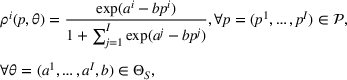
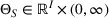
The seller's objective is to set a price
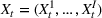
in each period t to maximize the total expected revenue over a selling horizon of T periods. Without knowing the true values of the parameters, the seller needs to learn from sales data. We adopt a Bayesian setting for demand learning. For each product i, the seller starts with a prior distribution
on
. After setting price
and observing sales
in period t, the seller updates the belief and obtains the posterior distribution
using Bayes' rule:
We note that there is no demand correlation among different products, so the sale of product
does not help with the learning of parameter
. In Section 4, we extend our model and consider a multinomial logit model, which allows us to incorporate demand correlation among different products.
Given the underlying demand parameters
, we can express the one‐period expected revenue as
. If the underlying parameters are known, the seller would simply set the optimal price that maximizes
and obtain a revenue of
in each period. We assume for simplicity that the optimal price of the underlying demand model is unique, which we denote by
. We further assume that
is an interior point of the set
and the Hessian matrix
of
is invertible. These assumptions are standard in the dynamic pricing and learning literature (e.g., Broder & Rusmevichientong, 2012; Keskin & Zeevi, 2014).
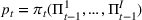
We define a policy as a sequence
, where
maps the historical price and sale pairs up to
into the price space
. In particular, a seller following a Bayesian policy π chooses the price
in period t. We use
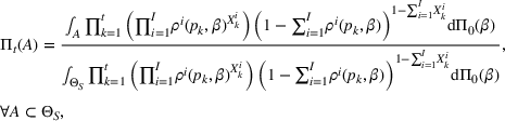
and
to denote the probability measure and expectation under policy π given the underlying demand parameter
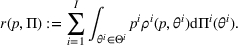
. To measure the performance of a policy π, we define the regret over a selling horizon of T periods as
Note that it is the cumulative expected revenue loss over T periods due to demand uncertainty.
Problem of incomplete learning
To achieve the maximum possible revenue, the seller would ideally learn the underlying demand model at some finite period and choose the optimal price from then on. Unfortunately, this is not possible due to demand uncertainty, and worse still, the seller may never learn the underlying demand model for some products, which is the problem of incomplete learning. We discuss how incomplete learning occurs in our setting.
For a product i, suppose there exists a price vector
that satisfies
for all
and some constant
. This price vector gives no information about telling apart different demand models for product i, and we call it an uninformative price. If a Bayesian policy π offers
, which implies that the belief will not be updated if the uninformative price is chosen. In the dynamic pricing problem of the single product i, any stationary policy will choose the same price in the next period, that is,
. Moreover, the same process will repeat in any period
, which implies that the seller will keep choosing the price
and never learn the underlying demand model for product i. In our problem with multiple products, recall that the selected prices depend on the posterior beliefs of all products, and we have
Although the posterior of a different product
is likely to be updated (i.e.,
),
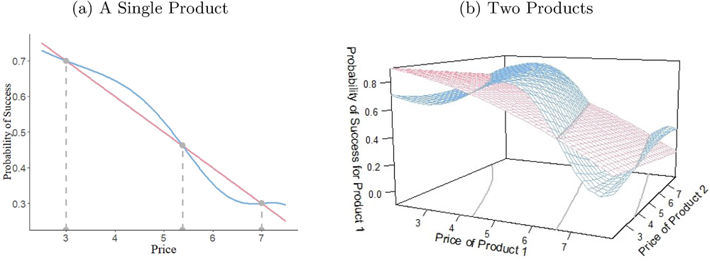
may be selected, especially after other parameters are learned sufficiently and their posterior distributions remain concentrated on the true values. Moreover, there can be an uncountable number of uninformative prices, and thus, the problem of incomplete learning is more common. To see that, consider two demand models for a product, and there is a one‐to‐one correspondence between the uninformative prices and the intersection points between two demand curves. Even in a single‐product problem, there can be multiple intersection points between two demand models, as shown in Figure 1a. If we incorporate multiple products, the intersection between two demand models becomes a collection of hypersurfaces in the high‐dimensional space. Figure 1b shows an example with two products: The demand models are surfaces in the three‐dimensional space, and their intersection is a collection of curves rather than isolated points.
Examples of two demand models. Note: In Panel (a), each curve corresponds to a potential demand model. There are three intersection points between the two demand models, and their projection in the one‐dimensional price space is a set of three discrete points. In Panel (b), each demand model depends on prices of the two products. Their intersection includes an uncountable number of intersection points. As shown in gray, the projection of the intersection points in the two‐dimensional price space is a collection of three curves.
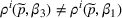
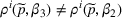
Now consider a price vector
that satisfies
for some pair of demand parameters
. It provides no information to distinguish between the demand models
and
, and we call it a confounding price. We note that all uninformative prices are confounding. However, if there is a parameter
such that
(or equivalently,
), the confounding price
may provide information to learn the difference between
may not cause incomplete learning. However, this is not true in general, as shown in the example in Appendix A.1 in the Supporting Information.
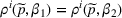
In contrast to a confounding price, we call a price
discriminative if it is mapped into distinct values by any pair of demand models, that is,
for any product i and any pair of parameters β1 and β2. This gives us a partition of the price space: the confounding prices (including the uninformative prices) and the discriminative prices. We note that discriminative prices may not exist for the continuous parameter case since there is an infinite number of potential parameters. Any discriminative price (if it exists) gives information to tell apart any pair of demand models, and it is therefore useful for learning. However, the seller may not choose it if it deviates from the best‐guess price under the current belief. This raises the trade‐off between learning and earning.
The problem of incomplete learning is more nuanced than our discussion above. If p is discriminative, but
and
are close for some
, then the amount of information we gather for learning may be limited. It can particularly be problematic if the optimal price of the underlying demand model happens to be uninformative. As an algorithm iteratively selects prices that converge to this optimal price, we obtain increasingly limited learning from sales data. This calls for a careful shrinking of how much the algorithm explores to strike the balance of learning and earning. In the Bayesian‐dithering approach we take, the balance of learning and earning is mediated by controlling the neighborhood size of dithering, as we will explain later.
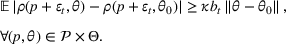
Before formally introducing dithering policies, we present an assumption essential for learning. As stated below, we assume throughout the paper that demand models are sufficiently distinct. More specifically, we assume that the underlying demand model
differs in the derivative (with respect to price) from any other demand model
around their intersection points.
For any product
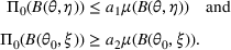
, we make the following assumptions:
For any
and any
, if
and
, then
When
is compact and convex, assume that for any
and any unit vector
, if
, then
where 0 is the zero vector in
.
Assumption 1 guarantees that parameters can be learned by pricing properly. As discussed above, any confounding price may cause the problem of incomplete learning, and intuitively, the underlying demand model should differ from any other demand model around the confounding prices so that it is possible to tell the difference between the two. This is guaranteed by Assumption 1(a). When the parameter is close to the underlying parameter θ0, the two corresponding demand models are close by continuity. It is harder to learn around their intersection, especially when the demand model is “flat” at θ0. Assumption 1(b) ensures that as prices vary, the demand model can become steeper at θ0. This implies that by perturbing the price, we can gather sufficient information and avoid incomplete learning at the intersection point. Assumption 1 is a technical assumption. We note that the assumption is satisfied by a wide range of parametric demand models commonly used in the pricing literature, such as the linear demand model
and the logit model
for
. It also rules out the unlearnable case such as
for
, where by varying prices we can only learn the sum
rather than the true value of each parameter.
Another typical assumption in the literature is the existence of k exploration prices such that if these prices are chosen in k consecutive periods, the corresponding distributions are different under any pair of different parameters (see, e.g., Broder & Rusmevichientong, 2012). This implies that the k exploration prices should be informative for any pair of models, yet any pair of demand models can be close or even overlap around the confounding prices. In that regard, Assumption 1 seems to be more restricted. Nevertheless, the exploration prices need to be identified in advance, which may be impractical since the number k can be large. For example, the linear model of I products requires
exploration prices, as discussed in Chen et al. (2021). They also mention that different choices of the exploration prices affect the empirical convergence rate in estimation, despite the same asymptotic rate. Thus, the exploration prices should be carefully chosen for the corresponding policy to perform well empirically.
Dithering policies
The myopic policy has been widely used in practice due to its simplicity (Morel et al., 2003). Since the problem of incomplete learning may occur under the myopic policy (Section 2.1), we modify it and propose dithering policies that achieve asymptotically optimal performance.
We start by introducing the MBP. For a seller who has beliefs
and chooses price
, the one‐period expected revenue is given by
Under the MBP, the seller chooses the best‐guess price
that maximizes the one‐period expected revenue, that is,
We note that the myopic price
may not be unique, and it may fall into the boundary of our price set
. However, as the posterior distribution converges to the underlying parameter, the myopic price tends to be unique and interior to
. This is because it gets closer to the optimal price that is assumed to be unique and interior to
We apply the dithering approach to modify the MBP. The idea is that by adding a perturbation to the myopic price, we can avoid confounding prices and gather sufficient information for learning with a high probability. More specifically, Bayesian dithering offers a chance to learn from a set of prices rather than a single one whenever making a pricing decision. As long as the set of confounding prices has measure zero in the price space, there is a high chance to choose a price that yields a sufficiently large gap between any pair of demand models, which helps tell them apart. For example, consider the example of two demand models for a single product in Figure 1a. Every time, the dithering policy chooses randomly from an interval of prices rather than a single price, and the seller can gather information from the difference between two demand models in a region. Whether it contains confounding prices or not, learning from a region offers a high chance of sufficient price exploration. Similarly, we can consider the example with two products in Figure 1b. There are an uncountable number of intersection points between two demand models of a product. However, if we choose from an interval of prices for each product, our choice provides sufficient information for demand learning with high probability.
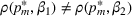
In this paper, we consider a policy
where the seller perturbs around the myopic price. We call this policy the dithering policy. In every period t, the dithering policy adds a perturbation
to the myopic price, that is,
, where
is the posterior distribution in the last period. We assume that
is uniformly distributed on the set
(i.e.,
), where
is a positive and decreasing sequence that converges to 0 as
. Our goal is to find the optimal price within
, but we allow the price vector to fall into a slightly larger space
after the perturbation. As the amount of perturbation shrinks over time, the price will eventually fall into
. Define d0 as the L2‐distance between
and the boundary
of
, that is,
. We assume that
is compact and convex and satisfies
. The dithering levels will be chosen such that any perturbed quantity is in
, as we shall see later. We further assume that all properties of the demand models
extend to
, including smoothness, boundedness, and Assumption 1 (this can be achieved by carefully extending the functions on
).
The choice of dithering levels
reflects the trade‐off between learning and earning: It controls the amount of price exploration, and a larger amount provides more information but less immediate revenue. Dithering is performed even if the myopic price is far from the confounding prices, which may incur unnecessary revenue loss. By carefully tuning
, however, we can control the cost, and our policy can achieve the asymptotically optimal performance, as we shall see in Section 3. This suggests that the performance of the myopic policy can be improved by dithering properly. We are aware of two recent papers, Qiang and Bayati (2016) and Bastani et al. (2021), that show the asymptotically optimal performance of the myopic policy in the presence of covariates. Similar to dithering, incorporating covariates also induces price variations to activate learning. However, it requires certain conditions for the myopic policy to avoid incomplete learning (e.g., covariate diversity in Bastani et al., 2021). In the general setting, we still need some control such as dithering to provide sufficient price variations and therefore avoid incomplete learning.
As a variant of the widely used myopic policy, the dithering policy is easy to implement and computationally efficient. Our dithering policy is an example of a randomized policy, which, in the context of dynamic pricing, can have practical benefits. For example, a policy that randomizes markdowns over time, compared to a state‐contingent policy, benefits retailers when online customers monitor the timing of purchase to obtain discounts (as shown in Moon et al., 2018). Similarly, the dithering approach makes it harder for monitoring and should be useful for pricing in the presence of strategic customers. Another property of the dithering policy is that price jumps vanish over time. In practice, this is desirable, as price fluctuation may affect customers' reference price or hurt the seller's reputation, which induces more uncertainty in demand and makes it harder to learn. We note that this property is also satisfied by the myopic policy, but it does not hold in many machine learning algorithms such as the ε‐greedy algorithm (see Auer et al., 2002). In particular, while the ε‐greedy algorithm does induce convergence of the posterior beliefs, jumps in the price sequence persist over time. We further illustrate this property by plotting the price paths under the myopic, ε‐greedy, and dithering policies, which can be found in Appendix A.2 in the Supporting Information.
Comparison with other policies
Before we proceed to the theoretical analysis, we compare our dithering policy with several typical policies studied in the literature and test their numerical performance in two examples.
MBP. As a baseline, we consider the MBP, which is widely used in practice (Morel et al., 2003). As discussed in Section 2.1, since it is a policy of pure exploitation, it may lead to the problem of incomplete learning and incur a considerable regret.
TS. A well‐known algorithm is TS, which has been shown to achieve a matching upper bound of order
in the classic MAB problem (Agrawal & Goyal, 2012) and applied in many dynamic pricing problems (see, e.g., Ferreira et al., 2018). While the dithering policy actively “tunes” its parameters to learn, TS explores in a passive way. In particular, it estimates the parameter by a sample from the current belief and chooses the corresponding optimal price. By sampling over the parameter space, TS also chooses a random price, but the passive way of learning may incur an extra regret when active exploration is not needed (as we shall see in Figure 2b).
FMBP. The flexibly constrained variant of the MBP (FMBP) is introduced in Harrison et al. (2012). It chooses the best‐guess price outside a predetermined interval of the confounding price with size
in period t. This requires solving a (nonconvex) constrained maximization in each period. One can implement this by projecting the myopic price onto the boundary if it is within a neighborhood of a confounding price and following the myopic price otherwise. We note that FMBP is designed and analyzed for the discriminative case, where the interval size should be set as
for
and a small
to achieve a constant regret. We can extend it to the finite parameter case and tune the constants α and ε1 for a good performance. For the continuous parameter case and the multiproduct problem, however, there can be an uncountable number of confounding prices, rendering it impractical to identify those prices and rule out their neighborhoods.
Controlled variance policy (CVP). The CVP is proposed in den Boer and Zwart (2014). To guarantee sufficient price exploration, it excludes a taboo interval centered at the average price and solves for the best price based on the maximum quasi‐likelihood estimate (MQLE). The taboo interval is designed with size
such that the variance of prices is lower bounded by
for some constants
and
. They tune the constants and analyze the theoretical performance of CVP for the generalized linear model, where the two unknown parameters are from a connected set similar to our continuous parameter case.
The CVP can be adapted to our Bernoulli‐demand setting with a linear form of selling probabilities, but the interval size should be adjusted when the parameter set is finite. For example, we adjust the lower bound as
for the finite parameter case, otherwise the cumulative regret would be of a higher order than
. (This is because the cumulative regret under CVP is proportional to
, where
is the average price.) Similarly, for the discriminative case, the lower bound should be adjusted as
to achieve a constant regret. Indeed, the size of the taboo interval would then become 0, and the CVP policy reduces to the greedy policy (Greedy) that chooses the optimal price under the “most likely” demand model, which corresponds to the parameter with the highest likelihood. We conjecture that the CVP policy with the above choices of the interval size would achieve matching upper bounds for the finite parameter case, but more work is needed to prove the theoretical performance. Besides, extending it to multiple products is not straightforward since the price variations should be guaranteed in different directions of the high‐dimensional price space (see the discussion in Keskin & Zeevi, 2014). We also note that CVP may need to solve a constrained maximization problem in each period, which is nonconvex in general. To avoid the potential computational issue, one can compute the myopic price based on the current estimate and project it onto the boundary of the taboo interval if it is outside the interval.
Average relative regret under different policies. Note: Each curve depicts the average relative regret of a policy over 104 sample paths. In Panel (a), we plot
versus T over 2000 periods. In Panel (b), we plot
versus
over 104 periods (the first 50 periods are omitted). Details of the examples and tuning parameters are provided in Appendix A.3 in the Supporting Information.
Now we compare the numerical performance of these policies. We first adopt the numerical example tested in Harrison et al. (2012), where FMBP can achieve a constant regret. Indeed, this example belongs to the discriminative case in which all optimal prices are discriminative, and a constant regret can also be achieved by a modified version of dithering (as we shall see in Section 3.3). In Figure 2b we plot the average relative regret, defined as
, where
and
are the cumulative regret and the optimal expected revenue when
is the underlying model. We observe that while MBP performs poorly due to incomplete learning, all other policies achieve a constant regret, among which dithering performs best. We note that TS and greedy exploit the information that there are only two possible optimal prices and restrict the selected prices to these two prices, and the passive way of learning under TS induces an extra cost of exploration compared to greedy. Since both optimal prices are discriminative and useful for learning, greedy performs well. For the general finite parameter case, however, the optimal price of a potential model can be confounding, and thus, it may be more likely to get into the problem of incomplete learning if we limit to the optimal price set.
We then extend to the finite parameter case, where the optimal price of a potential demand model can be confounding and the best achievable regret is of order
. In Figure 2a, we plot the average relative regret under MBP, TS, FMBP, CVP, and dithering. We can see that the average relative regret of dithering, TS, and FMBP is of order
. While CVP performs worse, it outperforms MBP that involves pure exploitation and may “get stuck” in the confounding price.
The numerical results shown in Figure 2 suggest that dithering performs close to FMBP for the discriminative case and TS for the finite parameter case, which have been shown to be asymptotically optimal for their corresponding case. In the following section, we will justify its good numerical performance for both cases. Furthermore, we will show that with carefully chosen dithering levels, our policy yields a matching regret upper bound for the continuous parameter case.
PERFORMANCE ANALYSIS: A SINGLE‐PRODUCT PROBLEM
In this section, we focus on the simple problem with a single product, that is,
. We call it the single‐product problem. The general problem with multiple products will be discussed in Section 4. We study a structural property of dithering, which demonstrates the role of dithering in price exploration (Section 3.1). Using the property, we illustrate the choices of dithering levels and derive a matching upper bound of the dithering policy for each of the following three cases: the finite parameter case (Section 3.2), the discriminative case in which the optimal prices of all finite number of potential demand models are known to be discriminative (Section 3.3), and the continuous parameter case (Section 3.4). For simplicity, we ignore the product index i.
A structural property of dithering
We first derive a structural property of the demand model when we apply the dithering approach. This result shows how dithering activates learning, which we will use to establish an upper bound on the rate of learning under the dithering policy.
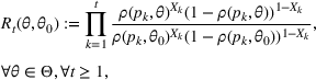
Let θ0 be the underlying parameter, and let
be a uniform perturbation on
. There exist constants
and
such that if
, the demand model satisfies
The intuition behind the proof is that since any pair of demand models
and
have different derivatives at their intersection points (Assumption 1), their relative difference
should be sufficiently large on most of the price space. For any price at which two demand models are close, it falls into a small neighborhood around some confounding price. By Assumption 1, the difference between their derivatives should be relatively large. More specifically, we can find constants
and
such that for any
, at least one of the following holds:
The above inequalities imply that Bayesian dithering that adds a random perturbation to a price can induce a larger relative difference between the two demand models
and
. It also explains why the lower bound in the statement of the lemma depends on the dithering level
. The detailed construction of c, κ, and b0 can be found in Appendix B in the Supporting Information. We note that Lemma 1 is an extension of the sublevel set estimates in Carbery et al. (1999), where a function with large derivatives on its domain has been discussed. In contrast, we only require that the derivatives are relatively large around the zero points of the function
.
Assumption 1 implies that the underlying demand model differs from any other model at their intersection. Based on the assumption, Lemma 1 shows the role of dithering in our policy: The perturbation guarantees that the mean relative difference between the underlying model and any other model is bounded away from zero, which implies that we can always gather some information about the underlying demand model and avoid incomplete learning. Moreover, the amount of information we gather depends on the dithering level, so we need to carefully tune it to strike a balance between learning and earning. In the following subsections, we will apply the structural property of dithering and tune the dithering level to bound the regret, when the parameter set is finite (the finite parameter and discriminative cases) and when it is compact and convex (the continuous parameter case).
The finite parameter case: An
upper bound on regret
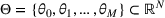
We now consider the finite parameter case, in which there are a finite number of potential parameters. We denote the parameter set by
, and θ0 is the underlying parameter vector. By an abuse of notation, we denote by
the posterior (or prior) mass on the parameter
for any
and any t. Throughout this subsection, we assume that the prior mass on the underlying parameter
is strictly positive so that it is possible to learn in a Bayesian way. We provide an
upper bound on the regret for our dithering policy, which matches the lowest achievable bound
To bound the regret from above, we show that by dithering properly, we can gather sufficient information in each period and learn the parameter at a reasonably fast rate. As we learn over time, the posterior distribution assigns more mass to the true value θ0, and the myopic price based on the posterior gets closer to the optimal price. This implies that the revenue loss from the myopic decision decreases to zero. Since the dithering level shrinks over time, the cost of dithering also decreases to zero. Thus, the one‐period regret under the dithering policy, which attributes to both the myopic decision and dithering, will eventually shrink to zero. Moreover, if the dithering level is suitably chosen, the cumulative regret can be bounded above by a term of order
.
Based on the idea above, we now formally establish the
regret bound for the dithering policy. First, we estimate how the posterior mass evolves. For a pricing policy to perform well, the likelihood function on any parameter
should decrease as more data are gathered, and the posterior
on the underlying parameter should converge to 1 at a reasonably fast rate. To bound the rate of learning
, we analyze the likelihood ratio between any parameter θ and the underlying one θ0, which is a random variable formally defined below:
where the randomness of
comes from the data
and prices
. We note that
is the ratio between the likelihood functions of θ and θ0. If
, we have
for any
. For any
, we expect
to decrease to zero as we learn gradually from the data that θ is less likely to be the true value compared to θ0. In the following lemma, we combine Lemma 1 and an information inequality to bound the term
, which estimates how the likelihood function on θ decreases compared to θ0. This will be further used to bound the rate of learning.
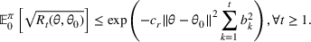
Let π be a dithering policy, and let b0 be the positive constant defined in Lemma 1. Then, there exists a constant
such that for any decreasing sequence
with
, the likelihood ratio satisfies
Lemma 2 says that the likelihood ratio associated with
decreases exponentially as we learn more about the parameter. The decreasing rate is faster if the total level of dithering
is larger, which indicates the role of dithering for learning. Also, if θ is closer to θ0, it is harder to learn, and the decreasing rate becomes slower. We note that a similar proof method has been used in Borovkov (1998) to estimate the likelihood ratio given independent and identically distributed (i.i.d.) data. Broder and Rusmevichientong (2012) extend their result to incorporate non‐i.i.d. data. However, they consider deterministic policies while we consider randomized policies given non‐i.i.d. data, which requires us to check whether the expectation over all possible price
given the data can be carried into the final exponential term.
, which captures how fast the posterior belief converges to the underlying parameter.Rate of Learning for the Finite Parameter Case
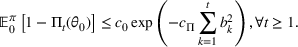
Let π be a dithering policy, and let b0 be the positive constant defined in Lemma 1. There exist constants
and
such that for any decreasing sequence
with
,
Theorem 1 presents the relationship between dithering levels and the rate of learning: A larger amount of dithering leads to a faster rate of learning, and the rate depends exponentially on the cumulative amount of dithering. Intuitively, dithering enables us to choose prices sufficiently far from the confounding prices with a high probability, which provides sufficient information to learn the underlying demand model. The proof comes from the observation that the posterior belief on θ0 is small only when the likelihood ratio for some
is large, which by Lemma 2, happens with a small probability. This provides an exponential upper bound on the rate of learning. Details of the proof can be found in Appendix C in the Supporting Information.
We note that constants
and c0 depend on M. Thus, these constants depend on the number of potential parameters. As the potential parameter set grows, the upper bound on the rate of learning becomes larger, which captures the increasing difficulty of learning. We also note that if the seller assigns more prior mass to the true value θ0, one would expect a smaller c0, which indicates the value of preliminary information incorporated in the prior.
We then make use of the rate of learning to establish an upper bound on the regret
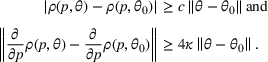
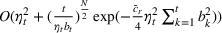
, which is defined in (2). In the following theorem, we bound the one‐period expected revenue loss above by the following two terms:
for some constant
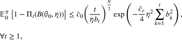
. The first term in the bracket is the (squared) myopic price deviation, which depends on how accurate the posterior belief is. The second term is the cost of dithering, which is controlled by the chosen level of dithering in that period. Thus, the rate of learning and the dithering level can be used to bound the one‐period expected revenue loss, which establishes the following upper bound on the regret.Regret Bound for the Finite Parameter Case
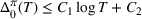
For any
, let
for all
, where
is a constant such that
, and
and b0 are defined in Theorem 1 and Lemma 1, respectively. Then, for a dithering policy π with dithering levels
, there exist finite constants C1 and C2 such that
for any
.
The choice of dithering levels
in Theorem 2 balances the trade‐off between exploration and exploitation. A larger amount of dithering leads to a faster rate of learning (Theorem 1), whereas it incurs a greater revenue loss due to deviation from the myopic price that converges to the optimal price. In our problem, we allow multiple intersection points of the two demand models and the possibility that the confounding price is optimal under some parameter. This requires a reasonable amount of price exploration to avoid getting “stuck” and maintain a relatively low cost in earning. The above theorem provides choices of
to meet the requirement. We note that
only depends on the given information (including the parameter set Θ and the range
of the demand models). However, the sequence
of dithering levels should be chosen from (0, b0), where b0, as defined in Lemma 1, depends mainly on the properties of the demand model around the confounding prices. In practice, we can start with a reasonable b1 and take
for all
. Since the decreasing sequence will eventually become smaller than b0, one can apply whatever we do here from that period on, and the performance guarantee still holds. We also note that the upper bound
is the best achievable bound of any pricing policy for the finite parameter case, which has been shown in Cheung et al. (2017). They also propose a policy with a matching upper bound, under which prices for exploration are chosen to activate learning. A discussion about their paper can be found in Section 1.1.
Under our policy, dithering enables us to avoid incomplete learning, but it also induces a revenue loss, which is the cost of learning. This cost can be reduced if we know in advance that the optimal prices of all potential demand models are discriminative, as discussed in the next subsection.
The discriminative case: A constant regret bound
Now we consider a special case of the finite parameter case, in which we know in advance that the optimal price of any demand model is discriminative. We call it the discriminative case. The parameter set is
, and we denote by
the optimal price if the underlying parameter vector is
. Then, the assumption for the discriminative case can be expressed as follows: For any
, the optimal price
satisfies
for any
. In that case, the dithering policy can be modified to achieve a constant bound on regret. We note that this case has been considered in Harrison et al. (2012) and Cheung et al. (2017).
As discussed in Section 2.1, it is difficult to learn from prices around a confounding price, and we add perturbation in each period to increase the chance of learning. Unlike the finite parameter case, there is no need to dither in every period given the prior knowledge that the optimal prices are discriminative. We can dither only when the selected price p is close to one of the confounding prices, which is depicted by the small relative difference
for some pair of parameters
and
. More specifically, consider a modified version of the dithering policy, π, as follows: Given the prior probability
at the beginning of period t, the selected price is
, where
Note that
is the myopic price as defined in (7), and parameter κ is given in Lemma 1. We call it the modified dithering policy.
We can make use of the results in Section 3.2 to show a constant bound on regret for the modified dithering policy. Intuitively, dithering enables us to learn without getting “stuck,” and after we gather sufficient information, the myopic price should be close to the optimal price with a high probability. Since the optimal price of the underlying demand model is discriminative, prices around the optimal price can provide information for learning, and there is no need to dither if these prices are chosen. Thus, we perform dithering less frequently, which reduces the cost of dithering and yields a constant regret, as formally shown below.Constant Regret Bound for the Discriminative Case
For any
and any
, let
for all
, where
is a constant such that
, and
and b0 are defined in Theorem 1 and Lemma 1, respectively. Then, for a modified dithering policy π with dithering levels
, there exists a finite constant C such that
for any
.
The proof is given in Appendix D in the Supporting Information. It takes a similar approach to Theorem 2 for the finite parameter case, but it requires some modifications. As shown in (13), we bound the one‐period regret by the myopic price deviation and the cost of dithering. The difference lies in the estimate of the cost of dithering, which we bound by the rate of learning, rather than the dithering level as in Theorem 2. Under the modified dithering policy in (14), no dithering will be applied after we gather sufficient information, and the cost of dithering, therefore, depends only on the rate of learning. Recall that the myopic price deviation depends on how accurate the estimate is. It follows that the one‐period regret can be bounded above by the rate of learning. Since the same bound on the rate of learning as in Theorem 1 is guaranteed, we can tune the dithering levels to establish a constant bound on regret. Recall that for the finite parameter case, the dithering level
decays at a rate of
to balance the trade‐off between learning and earning. Given the additional information in the discriminative case,
can decay at a rate of
for any
and still balance learning and earning.
Theorem 3 relies on the assumption that all optimal prices are discriminative. If the assumption is violated, the optimal price
of some demand model
happens to be uninformative, or more general, confounding. In that case, the chosen prices need to be far away from
to gather enough information for learning while, for earning, they should not deviate much from the optimal price
in case the underlying parameter is
. To balance the trade‐off, any pricing policy incurs a substantial revenue loss. Thus, we cannot obtain the constant regret bound without the assumption. Moreover, any policy must incur a worst‐case regret of
We note that the discriminative case has been studied in Harrison et al. (2012). In particular, they consider the problem with binary demand models and a single uninformative price. They propose a discriminative policy, under which the seller chooses outside an interval of the uninformative price to avoid incomplete learning. The size of the interval controls the balance between learning and earning. They show that by carefully shrinking the size of the interval over time, the discriminative policy can achieve a constant regret bound. This approach can be extended to the finite parameter case. Although they do not show for this case, the discriminative policy can achieve the same performance guarantee as ours if the sizes of the interval are chosen properly. However, this approach cannot be applied directly to the continuous parameter case. Since there is an uncountable number of potential parameters, all prices may be confounding, and it is likely to get stuck in any one of them. Thus, we cannot simply rule out neighbors of these prices. In contrast, the dithering policy can achieve asymptotically optimal performance for the continuous parameter case, as shown in the following subsection.
The continuous parameter case: An
upper bound on regret
Now we consider the continuous parameter case, in which the parameter set Θ is compact and convex. Different from the finite parameter case, the parameter
can be arbitrarily close to the underlying parameter θ0, which makes it harder to distinguish θ0 from the others. As shown in Broder and Rusmevichientong (2012), the worst‐case regret of any pricing policy must be
. In this subsection, we show that the dithering policy is asymptotically optimal, in the sense that the upper bound
on its regret matches the lower bound up to a logarithmic factor.
We first present assumptions for the continuous parameter case, which are regularity conditions on the prior distribution
. Since the seller knows the parameter set Θ, we assume without loss of generality that the prior is distributed within Θ, which implies that
for any set
satisfying
. We also assume two more regularity conditions, as stated below. Denote by
the open ball at θ with radius η. Let
be the Lebesgue measure on
.
Regularity Conditions
There exist constants
and
such that for any
,
and
, the prior distribution satisfies
Assumption 2 is common in the Bayesian statistics literature. For example, it is satisfied by any continuous probability distribution whose density function is strictly positive at θ0. It rules out the “unlearnable” case where an infinite prior density is assigned to some
, or a zero prior density is assigned to θ0.
We now introduce how we establish the regret bound. As shown in (13), the one‐period regret can be bounded above by the myopic price deviation and the cost of dithering. As we add perturbation to prices and gather sufficient information for learning, our posterior distribution tends to concentrate on the true value θ0. Then the myopic price gets closer to the optimal price, which leads to a decreasing revenue loss from the myopic decision. We can bound the myopic price deviation by how fast the posterior distribution shrinks to θ0. The approach so far is the same as the finite parameter case, but we need to formalize this idea in the context of a continuous posterior distribution. In particular, the rate of learning is now captured by
, the expected value of the posterior distribution outside a small neighborhood
of θ0. A large amount of dithering can speed up the rate of learning, but at the same time, the resulting price deviates from the myopic price that maximizes the immediate revenue gain (earning), which induces a high cost of dithering. By tuning dithering levels
, our policy can balance the trade‐off between learning and earning and achieve the lowest achievable regret. Since it is harder to tell apart θ0 from its neighbors, one would expect a slower rate of learning and a higher cost of dithering, and the regret would have a higher order.
The idea is similar to the finite parameter case, but the proof is not a straightforward extension. The main difference lies in the analysis of the rate of learning. For the finite parameter case, we can simply estimate the posterior distribution on each potential parameter
through its likelihood ratio
, and gather together to bound the rate of learning
. However, for the continuous parameter case, we need to handle the aggregate effect of the uncountable number of parameters. We thus discretize the set
into small open balls, which are, in fact, a finite cover of the compact set
. By analyzing the posterior on each ball, we can establish an upper bound on the rate of learning
. Specifically, by the definitions of the posterior distribution in (1) and the likelihood ratio in (10), the posterior on a small ball
can be expressed as
To analyze
, we need to consider the numerator and denominator separately. Using a similar argument to Lemma 2, we can show that if
and δ is small enough, the likelihood ratios on
behave similarly to the likelihood ratio
at its center θ, which decreases at an exponential rate as we gather more information for learning. Besides, since the likelihood ratio of any neighbor of θ0 should be close to 1, if a reasonable prior is assigned (Assumption 2), the denominator can be bounded away from zero. Combining the analysis of the numerator and denominator, we can establish an upper bound on
for any ball
of the discretization, which together bounds the rate of learning from above. We note that the ball
and its discretization are introduced for analysis. To implement Bayesian dithering, we can update the posterior using Bayes' rule given in (1), and there is no need to know η or δ for each discretized ball.
Given the regularity conditions and the idea stated above, we proceed with the main steps of the proof. Since there is an uncountable number of parameters, the analysis of a single parameter in Lemma 2 is insufficient to bound the rate of learning. We need to extend the lemma to analyze the likelihood ratios on a small ball. More specifically, given a small ball
, we define the local average likelihood ratio as
Intuitively, the local average likelihood ratio
of a small ball
should be close to
, the likelihood ratio at its center θ. Recall from Lemma 2 that
decreases exponentially as we gather information from dithering. If δ is small enough, one would expect that
behaves similarly and
also decreases at an exponential rate. In fact, by applying Lemma 1 and an information inequality, we can show that
decreases as we learn from dithering, and the decreasing rate depends exponentially on both the total level of dithering and the gap between θ and θ0. This is formally stated below.
Let π be a dithering policy, and let b0 be the positive constant defined in Lemma 1. Then, there exist constants
and
such that for any decreasing sequence
with
and any open ball
, the local average likelihood ratio defined in (17) satisfies
The approach we take to prove Lemma 3 is similar to Lemma 2, except that we need to deal with a small ball
rather than a single point θ. The proof is given in Appendix E in the Supporting Information.
Based on the analysis of the local average likelihood ratio, we can estimate the posterior distribution on any small open ball that does not contain θ0. For any
, since the compact set
can be covered by a finite number of open balls, the estimate on each ball can be gathered together to bound the rate of learning
, which captures how the posterior outside a small neighborhood of the true value evolves over time.Rate of Learning for the Continuous Parameter Case
Let π be a dithering policy. There exists a finite constant
Theorem 4 shows that with a substantial amount of dithering, the posterior distribution over a small neighborhood of the underlying parameter converges to 1 in expectation, and the rate of learning decreases exponentially in the total level of dithering. The bound on the rate of learning is of a higher order (with respect to t) than the one for the finite parameter case (Theorem 1), which indicates the challenge in learning for the continuous parameter case. Theorem 4 also describes how the posterior distributes given a sequence of dithering levels: The posterior distribution tends to concentrate on the true value θ0, and its tails decay exponentially fast. As the small ball we analyze shrinks (i.e., η decreases), the upper bound increases since it is hard to tell apart θ0 from its neighbors. We note that the constant
can be smaller if the prior belief is more accurate (e.g., a2 or ξ0 is larger in Assumption 2). In that case, the posterior distribution concentrates more on θ0, which implies the value of preliminary information incorporated in the prior. We also note that the curse of dimensionality occurs even in the single‐product problem, as indicated by the factor
. The factor follows from the discretization of the parameter space Θ. In particular, it increases with the number of the discretized balls, which depends on the radius η and grows exponentially with the dimension N of Θ.
The main idea of the proof is as follows. Since
decreases exponentially (Lemma 3), we expect that if the ball
is far from the true value θ0, the (i) local average likelihood ratio of
should be much smaller compared to the (ii) local average likelihood ratio of a neighborhood around θ0. By applying Lemma 3 to bound (i) from above and establishing a lower bound on (ii), we show that the posterior on
decreases at an exponentially fast rate. Recall that the set
is compact. It can be covered by a finite number of small open balls, and the posterior on each of them can be bounded. Thus, we can estimate the posterior distribution on
and bound the rate of learning with dithering levels
and the radius η of the ball. We note that the bound increases with the number of the discretized balls, which implies that their sizes should be large if we want a small bound. However, the sizes should be small enough so that we can apply the analysis of the local average likelihood ratio in Lemma 3. Thus, we need to carefully choose the sizes of the discretized balls to obtain a reasonable bound on the rate of learning. Details of the proof are deferred to Appendix E in the Supporting Information.
Banjević and Kim (2019) also use discretization and bound the numerator and denominator separately to analyze the posterior under TS in a stochastic control problem. They consider the posterior over the Hellinger neighborhood (the neighborhood with respect to the Hellinger distance) and assume that the Hellinger distance between the likelihood functions of any two different parameters can be bounded away from 0. The Hellinger distance is not applicable in our setting since it is possible that the Hellinger distance between the likelihood functions of two different parameters is zero under some action (price). Thus, we consider the natural neighborhood (with respect to the L2‐norm) in the real space
instead. This requires us to apply the property of dithering in Lemma 1 to analyze the local average likelihood ratio (Lemma 3) and further estimate the posterior.
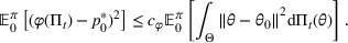
As shown in (13), the one‐period regret can be bounded above by the myopic price deviation and the cost of dithering. As we gather information over time, the posterior distribution tends to concentrate on the underlying parameter θ0, and the myopic price deviates less from the optimal price. Thus, we want to bound the myopic price deviation by the rate of learning to derive the regret bound. For the finite parameter case in Section 3.2, this can be achieved by applying the Implicit Function Theorem. However, now we need to deal with a continuous posterior distribution, for which the Implicit Function Theorem cannot be applied directly. We then introduce a property of the myopic policy, which bounds the myopic price deviation by the mean square error (MSE) of the posterior estimate.
There exists a constant
such that the myopic price under the posterior distribution
in any period
satisfies
We now apply Lemma 4 and Theorem 4 to derive the regret bound under the dithering policy. The posterior converges to θ0 at a faster rate as the total dithering level increases, but at the same time, dithering too much incurs a large revenue loss. This captures the tension between exploration and exploitation. By choosing a proper sequence of dithering levels, we can balance the trade‐off and further establish a regret bound of order
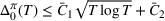
.Regret Bound for the Continuous Parameter Case
For any
, let
. Then, for a dithering policy π with dithering levels
, there exist finite constants
and
such that
for any
.
The proof of Theorem 5 is given in Appendix E in the Supporting Information. The high‐level idea shares some similarities as Theorem 2. Recall that the one‐period regret can be bounded above by two parts, the revenue loss from the myopic price and the cost of dithering. Lemma 4 shows that the revenue loss from the myopic decision based on
is dominated by the MSE of the parameter estimate. For any small
, the posterior over
should be small after sufficient learning, as shown in Theorem 4. Since
holds for any
, we derive that the MSE, and therefore the myopic price deviation, are
, where
should be carefully chosen to obtain a tight bound. Since the cost of dithering also depends on the dithering level, we can choose decreasing sequences
and
to establish a near‐optimal upper bound of order
on the one‐period regret. Hence, we obtain the
regret bound for the dithering policy, which matches (up to a logarithmic factor) the lower bound
) are also proposed by Broder and Rusmevichientong (2012) and Keskin and Zeevi (2014). The cycle‐based policy in Broder and Rusmevichientong (2012) chooses prices for exploration occasionally to explore. Keskin and Zeevi (2014) provide sufficient conditions for asymptotic optimality, under which learning is guaranteed by imposing an almost sure lower bound on the price variation up to each period. These conditions can be used to modify the myopic policy and balance learning and earning. In contrast, our dithering policy explores by adding perturbations to prices, and it does not satisfy the sufficient conditions in Keskin and Zeevi (2014). Moreover, these papers both consider a frequentist setting, while we take a Bayesian approach that allows us to incorporate prior knowledge (e.g., past experience) into our problem. We note that Broder and Rusmevichientong (2012) also discuss a well‐separated case in which the lower bound on the regret can be reduced to
. For the well‐separated case, the demand model satisfies
for some constant
. In that case, there is no need to add perturbation to prices, and a natural upper bound of order
can be achieved by the MBP, as a corollary of our analysis. (To see that, we can simply replace Lemma 1 with the property of the well‐separated case.)
EXTENSION TO MULTIPLE PRODUCTS
Let us consider the dynamic pricing and learning problem with multiple products. We refer to it as the multiproduct problem. Thus far, we have shown that by properly selecting the dithering levels, our policy is asymptotically optimal in the single‐product problem. In this section, we show that these results can be extended to the general problem with multiple products.
We first consider the case without demand correlation among products. Specifically, if the seller sets prices
, the demand of a product i follows a Bernoulli distribution with the selling probability
. Note that the demand model depends on the prices of all products, which may lead to an uncountable number of confounding prices even for the finite parameter case (as shown in Figure 1b). As such, the possible perturbation needs to span the price space to avoid getting stuck in a particular direction, which can be satisfied, for example, by our choice of the uniform perturbation
. As formally stated below, the dithering policy can also achieve matching regret bounds in the multiproduct problem without demand correlation.
Regret Bounds for the Multiproduct Problem
Let π be a dithering policy with perturbation
. For each of the following case, there exist a sequence of dithering levels
and finite constants
and
such that for any horizon
,
for the finite parameter case.
for the discriminative case.
for the continuous parameter case.
Our analysis for the single‐product problem can be applied directly to show Theorem 6. More specifically, recall from (13) that the one‐period regret under the dithering policy can be bounded by the (squared) myopic price deviation and the cost of dithering. For the multiproduct problem, the myopic price deviation comes from the parameter estimation error of each product. Since there is no correlation among products, the parameter vector of each product can be learned independently, and the posterior is updated as in (1). Thus, we can analyze the rate of learning for each product as in the single‐product problem. By gathering the analysis of the rate of learning, we can bound the myopic price deviation and then tune the dithering levels. Since the number of products is finite, we can obtain the same asymptotic regret bounds. Details of the proof are deferred to Appendix F in the Supporting Information.
Now, if there is a given correlation among products, the parameters would be learned based on the knowledge of the correlation. In that case, Bayesian dithering works, and our analysis can also be adapted to show similar performance bounds, which we will illustrate in a simple example below.
Let us consider a set of I substitutes. In each period, the realized demand
satisfies
. Moreover, one would expect shared parameters in the demand models. For example, we consider a multinomial logit (MNL) model of substitute products, in which the selling probability for a product i is given by
where
denotes the compact shared parameter set. Note that given the price vector p, the demands between any pair of products
are negatively correlated since their covariance is
. This model and its extensions have been widely adopted in the literature (see, e.g., Dong et al., 2009; Li & Huh, 2011). In contrast to the independent updating for each product in (1), the posterior of the shared parameter in period t would be updated using historical purchase decisions for all products, which by Bayes' rule is
where
captures the prior information at the beginning of the time horizon.
Based on the posterior, we can compute the myopic price and apply our dithering policy. Moreover, it can achieve regret bounds of the same order as in Theorem 6. This can be shown by adapting our analysis. Specifically, one can check that the demand model
for any product i satisfies Assumption 1, and thus, the structural property of dithering in Lemma 1 can be applied. Under the new updating rule in (22), dithering also serves to control the amount of information gathered in each period, and we can still bound the (local average) likelihood ratio in a similar way. Then, bounds on the rate of learning and the regret would follow directly. A more precise statement and the proof appear in Appendix F in the Supporting Information. We note that the one‐period expected revenue
is not necessarily concave in p, and the myopic price that maximizes
may not be efficiently computed. To avoid the computational issue, one can consider a variant that estimates the parameters by the mean or mode of the posterior distribution and solves for the myopically optimal price based on the estimate. Using (21), we can express the total revenue under a potential parameter vector as a function of the selling probabilities
. Moreover, it is jointly concave in ρ, as shown in Li and Huh (2011). Thus, the myopically optimal ρ can be solved efficiently, which uniquely determines the myopic price. For this variant, we can apply dithering, and our analysis can be adapted to show the regret performance.
The multiproduct problem has been studied by den Boer (2014) and Keskin and Zeevi (2014), where demands for products are assumed to be uncorrelated. The paper by den Boer (2014) considers parameter learning in a generalized linear demand distribution with known link functions and unknown parameters that determine the first and second moments. Their policy introduces a quadratic constraint to guarantee sufficient price exploration. They show a matching upper bound of order
for the so‐called canonical link functions that include Bernoulli distribution. Keskin and Zeevi (2014) study a linear demand model with sub‐Gaussian noises and provide sufficient conditions for designing asymptotically optimal policies. An idea of orthogonal pricing is introduced to guarantee that the chosen prices disperse in the price space. Both papers take a frequentist approach for parameter estimation, and the dimension N of the parameter space is a fixed function of the dimension I of the price space (i.e.,
or
). In contrast, we consider Bayesian learning for a Bernoulli‐distributed demand with a general form of demand functions, which requires significantly different analyses of the regret bounds. As a key distinction from the two papers above, our analysis extends to learning the classical MNL model, where demands for different products are correlated and parameters are shared across products. Moreover, we do not restrict the relationship between N and I. For example, there can be
parameters to learn for a quadratic demand model of the I‐dimensional price vector. This requires an additional analysis of the structure property of dithering to derive the matching regret bounds.
CONCLUSIONS AND FURTHER DISCUSSIONS
In this paper, we have studied the dynamic pricing and demand learning problem in a Bayesian setting. We have discussed the problem of incomplete learning in the general problem with multiple products. The main contribution of this paper is to present dithering as a unified approach to strike the balance between exploration and exploitation in the context of dynamic pricing. By analyzing the effect of dithering and the rate of learning, we prove that dithering policies are asymptotically optimal with respect to the regret for three classes of problems in the existing literature. Specifically, we take uniformly distributed perturbations as an example and show how to determine the dithering levels to achieve a matching upper bound on regret for each of the three problems. We establish an upper bound of order
for the finite parameter case, and under an additional assumption (the discriminative case), we show a constant regret bound for the modified dithering policy. For the continuous parameter case, we prove an upper bound of order
, which matches the existing lower bound (up to a logarithmic factor). Our work sheds light on the strengths of dithering in addressing incomplete learning. While we use uniformly distributed perturbations, other types of perturbations, discrete or continuous, will likely work as long as they provide sufficient price variations for learning. We believe the idea of dithering can be adopted to more complicated problems, such as pricing under inventory constraints (e.g., Ferreira et al., 2018) and learning in a changing environment (e.g., Keskin & Zeevi, 2016). Another contribution is our proof techniques in the Bayesian setting. Our analysis of the posterior and the regret bound works for general (parametric) price–demand curves and continuous price and parameter sets. We hope that the tools we introduce can facilitate further research about Bayesian learning in the dynamic pricing problem.
Bayesian and Frequentist. We take the Bayesian approach for learning, which allows us to account for prior information, such as domain knowledge from experts and market surveys. This is different from the frequentist approach. Also, certain priors can be viewed as regularizers in the parameter estimation problem to prevent overfitting (e.g., Murphy, 2012). Bayesian updating has been used and studied in a wide range of areas. There are many efficient simulation‐based methods, such as Markov chain Monte Carlo (e.g., Robert, 2007), which is of practical interest. We have shown that dithering can provide sufficient price variations to facilitate demand learning in a Bayesian setting. This introduces a challenge in analyzing the posterior distribution to bound the rate of learning, and our analysis may be of independent interest. We note that dithering can also be combined with a frequentist approach, such as the maximum likelihood estimation. We conjecture that the corresponding policy can still achieve the asymptotically optimal performance in terms of regret.
Model Extensions. The Bernoulli‐distributed demand considered in this paper can be extended to a binomial demand distribution, which covers applications in which we set a price for a number of customers before adjusting it. In particular, we can consider N customers coming in a period, observing the same price, and purchasing. Then, demand of any product i follows a binomial distribution with parameters N and
. We note that the posterior distribution in period t is the same if we follow the same pricing policy but fix a price for N consecutive periods under Bernoulli demand. Thus, our analysis of dithering policies and their performance can be carried over. A general demand distribution is beyond the scope of this paper; however, Bernoulli and binomial demand can approximate a large number of dynamic pricing and learning problems in practice.
We note that the dynamic pricing and learning problem falls into the category of online optimization with partial feedback (e.g., Russo & Van Roy, 2016). In this paper, we focus on the context of dynamic pricing as it is an important application in practice. We believe that the dithering approach can be applied to more online optimization problems, which we leave as future research.
Footnotes
ACKNOWLEDGMENTS
We thank the department editor, the senior editor, and two anonymous reviewers for their helpful and constructive suggestions, which have improved the paper significantly. The first author was partially supported by the Canada Research Chair Program and the Natural Sciences Engineering Research Council of Canada Discovery Grant (RGPIN‐2020‐04213). The second author was partially supported by the Natural Sciences Engineering Research Council of Canada Discovery Grant (RGPIN‐2015‐04019).
ORCID
Woonghee Tim Huh
Michael Jong Kim
Meichun Lin
References
1.
AgrawalS.GoyalN. (2012). Analysis of thompson sampling for the multi‐armed bandit problem. In Conference on learning theory (pp. 39–41). JMLR Workshop and Conference Proceedings.
2.
AuerP.Cesa‐BianchiN.FischerP. (2002). Finite‐time analysis of the multiarmed bandit problem. Machine Learning, 47, 235–256.
3.
BanjevićD.KimM. J. (2019). Thompson sampling for stochastic control: The continuous parameter case. IEEE Transactions on Automatic Control, 64(10), 4137–4152.
BorovkovA. A. (1998). Ergodicity and Stability of Stochastic Processes. Wiley, Chichster, U.K.
6.
BroderJ.RusmevichientongP. (2012). Dynamic pricing under a general parametric choice model. Operations Research, 60(4), 965–980.
7.
CarberyA.ChristM.WrightJ. (1999). Multidimensional van der Corput and sublevel set estimates. Journal of the American Mathematical Society, 12(4), 981–1015.
8.
ChenQ.JasinS.DuenyasI. (2021). Joint learning and optimization of multi‐product pricing with finite resource capacity and unknown demand parameters. Operations Research, 69(2), 560–573.
9.
CheungW. C.Simchi‐LeviD.WangH. (2017). Dynamic pricing and demand learning with limited price experimentation. Operations Research, 65(6), 1722–1731.
10.
denBoerA. V. (2014). Dynamic pricing with multiple products and partially specified demand distribution. Mathematics of Operations Research, 39(3), 863–888.
11.
denBoerA. V. (2015). Dynamic pricing and learning: Historical origins, current research, and new directions. Surveys in Operations Research and Management Science, 20(1), 1–18.
12.
denBoerA. V.ZwartB. (2014). Simultaneously learning and optimizing using controlled variance pricing. Management Science, 60(3), 770–783.
13.
DongL.KouvelisP.TianZ. (2009). Dynamic pricing and inventory control of substitute products. Manufacturing & Service Operations Management, 11(2), 317–339.
HarrisonJ. M.KeskinN. B.ZeeviA. (2012). Bayesian dynamic pricing policies: Learning and earning under a binary prior distribution. Management Science, 58(3), 570–586.
16.
KeskinN. B.ZeeviA. (2014). Dynamic pricing with an unknown demand model: Asymptotically optimal semi‐myopic policies. Operations Research, 62(5), 1142–1167.
17.
KeskinN. B.ZeeviA. (2016). Chasing demand: Learning and earning in a changing environment. Mathematics of Operations Research, 42(2), 277–307.
18.
LiH.HuhW. T. (2011). Pricing multiple products with the multinomial logit and nested logit models: Concavity and implications. Manufacturing & Service Operations Management, 13(4), 549–563.
19.
LoboM.BoydS. (2003). Pricing and learning with uncertain demand. In INFORMS revenue management conference. Working paper, Duke University, Durham, NC.