






Abstract
The results of an original calibration methodology that accounts for interelement influences in the analysis of alloyed steels using laser-induced breakdown spectroscopy (LIBS) are presented. The results were obtained from a dataset of spectra provided for the regression competition at the LIBS 2022 conference and available online. The dataset includes spectra from 41 steel samples with known concentrations of major alloying elements (chromium, nickel, manganese, molybdenum, carbon, silicon, copper) and 15 samples with unknown compositions for model validation. The concentration of alloying elements varies over a wide range, with iron content ranging from 98% to 41%. To reduce spectral line position instability, we applied a preprocessing method that maximizes the correlation of each spectrum with the first spectrum in the dataset. The implementation of the developed calibration methodology led to an improvement in the root mean square error of the analysis, with reduction factors ranging from two (for nickel and molybdenum) to five (for manganese and chromium) when compared to classical calibration.
This is a visual representation of the abstract.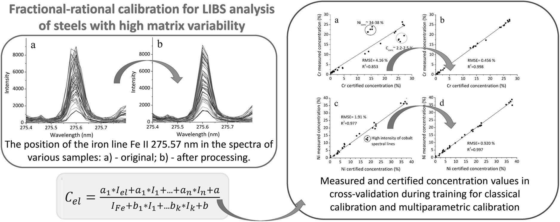
Keywords
Introduction
Laser-induced breakdown spectroscopy (LIBS) is a versatile analytical technique that utilizes a focused laser pulse to ablate a small amount of the sample surface, forming a microplasma. The emitted light from this plasma is then spectroscopically analyzed to determine the elemental composition of the material. 1 This process enables rapid, near-real-time analysis, usually involving only simple sample preparation. LIBS offers several distinct advantages over traditional analytical techniques. Primarily, it is a minimally destructive method, requiring only optical access to the sample, making it suitable for in situ and remote analyses, including on-line process monitoring 2 and molten material analysis. 3 It is capable of detecting virtually any element, including light elements such as hydrogen, 4 lithium, 5 and beryllium, 5 which are virtually impossible to detect using X-ray fluorescence (XRF) spectroscopy. Additionally, LIBS requires minimal sample preparation, reducing analysis time and cost. Finally, it provides rapid results, making it ideal for applications requiring high-throughput analysis. 6 Due to its unique capabilities, LIBS has found applications in a wide range of fields. In geology, it is used for mineral exploration and rock analysis. 7 Low destructiveness and high locality allow for mapping of elements in the analysis of historical and artistic values. 8 Furthermore, LIBS is increasingly used in recycling industries for rapid sorting and analysis of materials. 9 LIBS plays an important role in space exploration, enabling in-situ analysis of planetary surfaces and atmospheric composition. 10 The application of machine learning methods to LIBS enables not only elemental but also material separation based on molecular composition. 11 It is also employed in forensic science for rapid analysis of trace evidence, 12 contributing to criminal investigations. However, despite these advantages, achieving accurate quantitative analysis with LIBS remains a significant challenge.
Despite its numerous advantages, the quantitative accuracy of LIBS is generally lower compared to established techniques such as XRF and inductively coupled plasma optical emission spectroscopy (ICP-OES), primarily due to the inherent non-linearity of the signal response with respect to elemental concentration. This complexity stems not only from spectral interferences but also from a multitude of intricate matrix effects.
Conventional approaches based on increased spectral resolution or the selection of interference-free analytical lines are subject to practical limitations, as high-resolution spectrometers are often costly and bulky, which limits their applicability in many practical applications, and the choice of suitable spectral lines is limited by the availability of lines with adequate intensity, while the complex nature of laser-induced plasma and matrix effects results in non-linear relationships between spectral signal intensity and elemental concentration beyond direct spectral line overlap. Inter-element effects may arise from the influence of one element on the spectral radiation of another, caused, among other things, by changes in surface reflectivity, the formation of oxide layers, preferential segregation of elements at grain boundaries in metal alloys, changes in the thermophysical properties of the material, formation of various phases such as carbides, nitrides, intermetallic compounds, and solid solutions, fluctuations in plasma temperature and electron density when the material is enriched with easily ionized components, changes in surface roughness, etc. These effects are particularly pronounced in complex matrices such as alloys, where the presence of multiple elements can significantly alter the observed spectral intensities, hindering accurate quantification. Therefore, the development of robust calibration strategies that can effectively account for these inter-elemental influences is crucial for expanding the applicability of LIBS in quantitative analysis.
Constructing a relationship between signal intensity and the concentration of an element in a sample can be done in various ways. The simplest classical calibration approach is a linear function that relates intensity to concentration. In this case, the intensity of a spectral line is defined as the difference between the peak height and the background level measured at a control point. 13
Modern spectrometers are capable of recording extensive data on intensity distribution across the spectral range. However, such data are typically not utilized in the classical approach. To extract more comprehensive information from spectral data, machine learning methods can be applied, for example, partial least squares regression (PLSR), support vector machines (SVM), and artificial neural networks (ANN).1,9,11
Nevertheless, a significant portion of spectral data does not carry useful information. LIBS spectra of elements consist of sets of relatively narrow spectral lines, covering only small portions of the spectrum. The remaining regions mostly contribute to noise and increase the complexity of the model. Spectral data are usually high-dimensional, ranging from several thousand to several tens of thousands of spectral points, while the number of samples available for training typically does not exceed a few dozen. For instance, the spectra provided in Képeš et al. 1 contain 40 000 points and data for only 41 samples.
Variable selection algorithms can be more efficient in identifying non-obvious relationships between spectral regions and the analysis results.14,15 However, these algorithms require complex regularization techniques to avoid overfitting. This is particularly important when the number of training samples is significantly smaller than the number of original spectral variables, a common scenario in LIBS.
In Képeš et al., 1 one of the best results were achieved by the team that trained their neural network (NN) not on the full spectrum, but on narrow spectral regions containing analytical lines. These lines were identified using the National Institute of Standards and Technology (NIST) spectral database. 16 The dimensionality of the data used for NN training was reduced to about 3% of the original spectrum size, though it still significantly exceeded the number of samples in the dataset.
In this work, we propose a method based on constructing a multi-parameter function using the intensities of identified spectral lines. This approach does not use raw spectral data, but rather the classically measured intensities of spectral lines. To improve the accuracy of quantitative determination of alloying elements (chromium, nickel, manganese, molybdenum), calibration functions were constructed as rational expressions, where elemental concentration was modeled using linear combinations of spectral line intensities in both the numerator and denominator.
The efficacy of this novel approach was evaluated using a publicly available spectral dataset provided for the regression competition at the LIBS 2022 conference by Képeš et al. 1
Experimental
Material and Methods
This section provides the key specifications of the LIBS system used for spectral acquisition. A more detailed description of the experimental setup, data acquisition methodology, sample composition, and preparation procedures can be found in Képeš et al. 1 Plasma excitation was generated using a Q-switched neodymium-doped yttrium aluminum garnet (Nd:YAG) laser operating at a wavelength of 1064 nm, with a pulse duration of 10 nanoseconds and pulse energy 95 mJ. The laser beam was focused onto the sample surface to a spot diameter of approximately –0.2 mm. The emitted light from the laser-induced plasma was collected and analyzed using an echelle spectrometer with a cross-disperser, which provided a spectral resolving power of 6000 over a working spectral range of approximately 236 to 1000 nm. The detection of the plasma emission was temporally resolved with a delay of 1.5 μs after the laser pulse, and the signal was integrated over a gate width of 50 μs. For each sample, 50 individual LIBS spectra were recorded at different locations on the sample surface to enhance the representativeness of the data
For the training sample set, the authors 1 provided data on the content of chromium, nickel, manganese, molybdenum, carbon, silicon, and copper. The elemental concentrations in the training set varied within the following ranges: carbon 0.00913–3.04%, silicon 0.00188–2.3%, manganese 0.0582–6.57%, chromium 0.045–27.16%, molybdenum 0.00431–3.62%, nickel 0.0195–37.72%, copper 0.005–3.1%, and iron 41.49–98%.
Although sample pre-burn is frequently employed in LIBS to remove surface contaminants and improve stoichiometry,14,15,17,18 it was omitted from this study. The authors of Képeš et al., 1 from which the data for this study were obtained, utilized a different approach. They performed thorough mechanical cleaning of the sample surface and acquired each spectrum at a new location on the sample. This method offers several advantages. It ensures high representativeness of the data across the sample surface, contributing to more reliable analytical results. In addition, the method provides higher spectral intensities, likely due to more efficient ablation facilitated by the presence of surface micro-roughness. 19 Moreover, it allows obtaining a large number of individual spectra under constant analytical conditions. This aspect is particularly important for training multivariate models such as PLS, SVM, and ANN, which require extensive datasets to ensure robust and accurate performance.
However, this approach may potentially amplify inter-element effects related to surface phenomena. The surface composition may differ from the bulk material composition. Different metals exhibit varying tendencies to form oxide films. Furthermore, surface roughness after polishing can vary across samples due to differences in hardness of steels alloyed with various elements. Therefore, not all effects observed in this study may manifest with a different spectral preparation and spectral acquisition strategy.
Spectra Preprocessing and Calibration Model
The Matlab R2022b package from The MathWorks Inc. was used to build the calibration model and spectra preprocessing.
Operation of the spectrometer can be accompanied by a shift in spectral lines, caused by thermal or mechanical instability. To compensate for the aforementioned shift in the position of spectral lines in the spectral data, spline interpolation of the spectrum and a transformation of the wavelength scale were applied. This transformation included constant, linear, and quadratic terms, intended for the correction of shift, stretching, and non-uniform stretching, respectively. The transformation parameters were optimized by maximizing the correlation coefficient of the processed spectra with the first spectrum of the set, which contributed to increasing the stability of the position of the spectral components. This processing was applied to the spectral region spanning 236–440 nm, which contains the lines of all elements present in the sample, except for carbon. The carbon line was measured from the unprocessed spectrum. The proposed approach previously demonstrated its effectiveness in the analysis of low-alloy steels using a spectrometer built according to the Czerny–Turner scheme. 20 The obtained results Figure 1 indicate its applicability to the spectra of high-alloy steels as well, recorded with an echelle spectrometer with crossed dispersion, despite the synthetic nature of the provided linear spectra (obtained by combining sections recorded in different spectral orders) and a significant increase in the variability of the matrix composition.
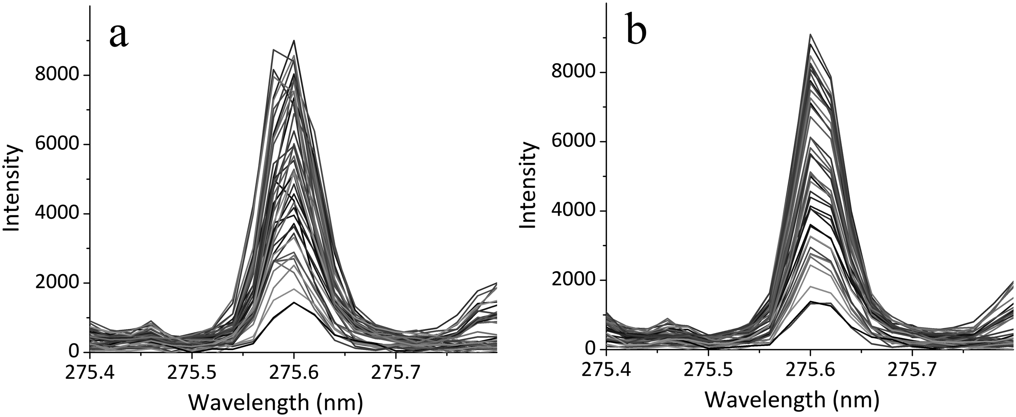
The position of the iron line Fe(II) 275.57 nm in the spectra of various samples: (a) original and (b) after processing.
Calibration curves were constructed as a function of:

The calibration procedure was implemented as a stepwise forward selection algorithm. Initially, the model included only the analytical line intensity and a constant term in the numerator, with the reference iron line in the denominator. Additional spectral lines were then iteratively tested for inclusion, alternately in the numerator and denominator. The optimization procedure followed these steps: (i) Each candidate line was temporarily added to the numerator; (ii) model coefficients were optimized using the Nelder–Mead 21 simplex algorithm by minimizing the cross-validated root mean square error (RMSE); (iii) each candidate line was temporarily added to the denominator; (iv) model coefficients were optimized using the Nelder–Mead simplex algorithm by minimizing the cross-validated RMSE; (v) the candidate line and its position (numerator or denominator) producing the largest RMSE reduction were permanently retained; and (vi) the procedure continued until either no improvement in RMSE was observed or the total number of calibration coefficients reached eight.
Although a commonly cited heuristic in multiparametric regression suggests on the order of ten samples per fitted parameter, the present model employs a relatively aggressive parameterization given the limited sample size. In this context, leave-one-out cross-validation (LOOCV) was used during the model development stage to obtain an exhaustive assessment of model generalization, with each sample serving sequentially as validation data. The resulting model was subsequently evaluated on an independent test set, providing an additional check against overfitting. Under this validation strategy and given the controlled model selection procedure, the number of fitted coefficients was limited to eight, representing a compromise between model flexibility and statistical stability under the constraints of the available dataset.
The adopted rational model structure inherently reduces the risk of denominator singularities, as the denominator includes a stable, non-zero contribution from a major matrix element (Fe). In addition, model parameters are estimated by minimization of the overall prediction error (RMSE) under a sequential model refinement procedure, which discourages configurations leading to vanishing denominators due to the associated increase in the loss function. Although numerical safeguards against division by zero (e.g., taking the absolute value of the denominator or adding a small positive constant) are in principle possible, they were not applied. During model construction, no instances of near-zero denominator values were observed for any spectral line listed in Table I.
Spectral lines of the calibrated elements and RMSE in cross-validation.
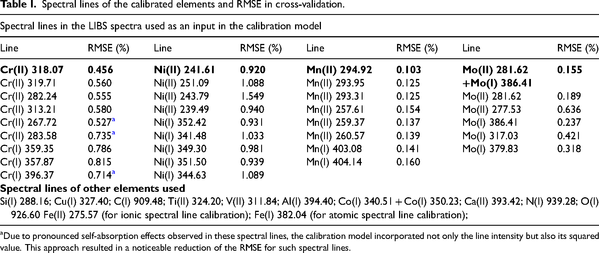
Due to pronounced self-absorption effects observed in these spectral lines, the calibration model incorporated not only the line intensity but also its squared value. This approach resulted in a noticeable reduction of the RMSE for such spectral lines.
This calibration strategy was selected by taking into account both potential spectral interferences that may affect either the analytical line or the reference iron line, and non-spectral effects, such as the reduced intensity of the iron line caused by surface depletion of iron when the sample becomes enriched with other alloying elements. The proposed method partially relies on ideas from the calibration-free approach of Ciucci et al. 22 and the single-sample calibration method of Yuan et al., 23 as both methods estimate relative concentrations through normalization to the sample’s total elemental composition. This consideration is particularly important for the present set of steels, in which the iron content—the major constituent—varies by more than a factor of two. Consequently, simple normalization to the iron line would be methodologically incorrect. However, as demonstrated in this study, unlike in Ciucci et al. 22 and Yuan et al., 23 the optimal denominator differs for each element, and the influence of individual components is not directly proportional to their concentrations in the alloy. The proposed model also shares certain similarities with the approach reported in Vrenegor et al. 24 However, in contrast to Vrenegor et al., 24 which compensates for inter-element effects based on known concentrations of all elements in the sample, the present model requires concentration data only for the target analyte.
Obviously, inter-element interactions are not limited to the considerations mentioned above; they are significantly more complex and diverse. This complexity makes it challenging to predict the exact form of the calibration function. However, incorporating spectral line intensities in both the numerator and the denominator expands the ability to account for these interactions and allows for more flexible modeling of their influence on the analytical signal.
In addition to the declared elements with known concentrations, spectral analysis in some samples revealed the presence of spectral lines for cobalt, vanadium, titanium, calcium, and aluminum. Tungsten might also be present, but its emission line is too weak to confirm with certainty. Some of these elements, such as calcium and aluminum, are common contaminants that are difficult to completely remove despite cleaning efforts. However, cobalt, vanadium, and tungsten are relatively rare elements and were likely present in the raw materials used to produce the samples. Spectral lines corresponding to nitrogen and oxygen, the main components of air, are also observed in the infrared (IR) region of spectra. The identification of spectral lines was carried out using the atomic spectral line database from CD-ROM 23 of R. L. Kurucz. 25 The Kurucz database contains transition probabilities and energy levels for a greater number of spectral lines than the NIST database, which, on average, allows for a more accurate estimation of relative line intensities during spectral line identification in LIBS plasma. In contrast, the relative line intensities provided in the NIST database are compiled from various authors and sources and are not normalized to a uniform scale.
Results and Discussion
Table I summarizes the spectral lines evaluated in this study, together with the RMSEs obtained via cross-validation for each line.
As shown in Table I, the spectrum contains a large number of chromium, nickel, and manganese lines of varying intensity, including both atomic and ionic transitions. In contrast, molybdenum is represented by only a few weak lines, offering limited selection. Due to the low intensity of molybdenum emissions, the two most intense lines were combined and treated as a single variable in the calibration. A similar approach was applied for cobalt.
The lines that yielded the best cross-validation results during the training phase are highlighted in bold in Table I. All subsequent analyses and results are based on these selected lines.
For each target element, several spectral lines were assessed, and the line demonstrating the best performance in cross-validation was selected for further analysis. In cases where an atomic line was employed for calibration, the Fe(I) 382.04 nm line was incorporated into the denominator; when an ionic line was selected, the Fe(II) 275.57 nm line was used accordingly. For other elements whose lines were detected in the spectrum, only a single line was used, preferentially selecting intense lines with minimal spectral interference.
Initially, it was intended to use both atomic and ionic emission lines of the calibrated element and iron to improve the representativeness of different plasma zones in the calibration models. However, the application of multiple lines for a single element often led to a significant increase in the number of iterations required for the optimization algorithm to converge, hindering the achievement of the optimum. It is likely that, in this case, the characteristic topology of the optimization function surface necessitates the application of an alternative algorithm. Consequently, a single analytical line was selected for the quantitative determination of each element.
Figure 2 and Table II demonstrate the significant improvement in calibration accuracy achieved using a multiparametric approach compared to classical univariate models. In the classical calibration Figures 2a,c, the predicted concentrations of chromium and nickel show considerable deviation from the certified values, particularly in specific compositional ranges. For chromium in Figure 2a, a notable deviation is observed for samples with high nickel content ∼34–38% and carbon content ∼2.2–2.5%, suggesting a compositional matrix effect. Similarly, in the case of nickel Figure 2c, systematic underestimation occurs in samples exhibiting strong cobalt line intensities. Importantly, these effects cannot be solely attributed to spectral overlap, as the cobalt and carbon lines are significantly weaker than those of chromium and nickel in the studied LIBS spectra. This points to more complex non-spectral matrix interferences.
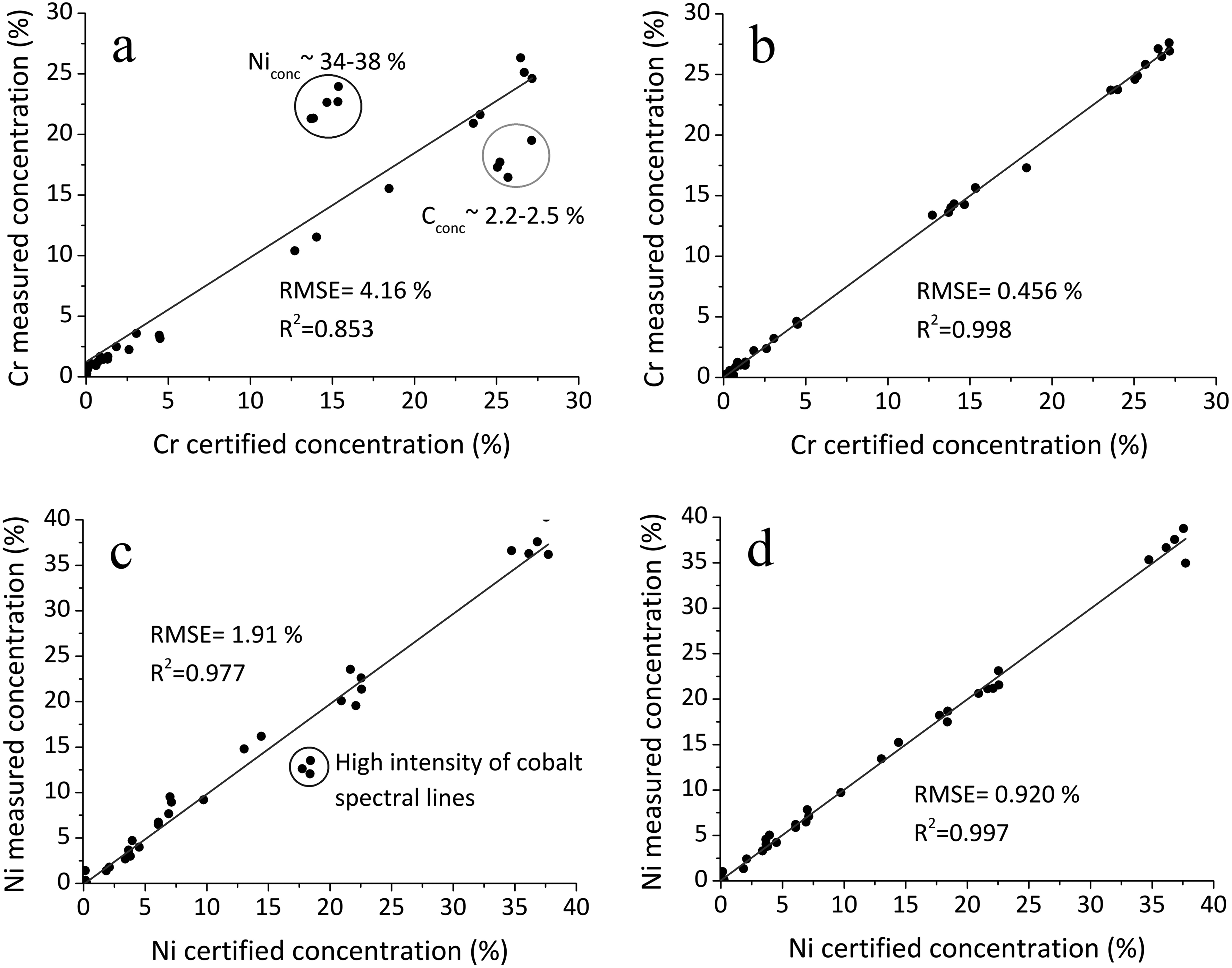
Measured and certified concentration values in cross-validation during training: (a) classical calibration using the chromium line Cr(II) 318.07 nm with normalization to the iron line Fe(II) 275.57 nm, (b) multiparametric calibration for chromium, (c) classical calibration using the nickel line Ni(II) 241.61 nm with normalization to the iron line Fe(II) 275.57 nm, and (d) multiparametric calibration for nickel.
Comparison of RMSE for different elements during cross-validation and on the test set using classical and multiparametric calibration approaches.

In contrast, the multiparametric calibration approach Figures 2b,d, which accounts for such matrix effects by incorporating additional spectral and compositional information, substantially reduces the RMSE. As summarized in Table II, the RMSE for chromium prediction during cross-validation decreased from 4.16%, with the classical approach to just 0.456% using the multiparametric model. A similar trend is observed for nickel, with RMSE reduced from 1.91% to 0.920%. Improvements are also evident for manganese and molybdenum, underscoring the robustness of the multiparametric calibration strategy across different elements.
As shown in Table II, a substantial difference between the RMSE obtained during cross-validation of multiparametric calibration and that observed on the test set is evident only for chromium. This discrepancy may be attributed to the significant influence of carbon Figure 2. The accuracy of carbon quantification under surface scanning conditions can be distorted by the presence of a thin film of organic compounds, which is difficult to remove without prior thermal treatment. Furthermore, only a single weak spectral line of carbon, C(I) 909.48 nm, was identified in the dataset.
In our previous work, 20 we demonstrated that even in cases where carbon lines are not clearly visible in steel spectra, its concentration can be estimated using PLSR based on spectra region near ionic carbon lines, i.e., C(II) 426.73 nm and C(II) 426.70 nm, under double-pulse spectra excitation. Alternatively, carbon can be quantified via the spectra region of CN molecular band in the 380–390 nm range when collecting emission from the trailing edge (tail) of a plasma plume generated by a passively Q-switched laser. 21 However, neither of these approaches proved effective for the current spectral dataset, likely due to differences in plasma excitation conditions and spectra detection parameters.
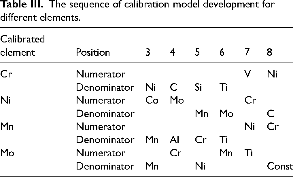
Table III presents the sequential incorporation of spectral variables into the calibration models for each target element. The table distinguishes between contributions to the numerator and denominator of the nonlinear regression function used in this study. Notably, elements present in high concentrations within the samples, such as chromium and nickel, do not always exert a proportionate influence on the calibration models of other elements. For instance, chromium is introduced only at later stages of the model for manganese, and nickel contributes to the molybdenum model only in a limited way.
The sequence of calibration model development for different elements.
These results differ in part from those reported in Vrenegor et al., 24 where the influence of matrix elements in the LIBS analysis of high-alloy steels was also investigated. In that study, nickel was found to be affected by chromium, molybdenum, titanium, and carbon; chromium by nickel and titanium; manganese primarily by titanium; and molybdenum by chromium, nickel, copper, and titanium. In addition to differences in the functional form used to account for inter-element effects, such discrepancies may also arise from several methodological and experimental differences between the studies.
Surface-Sensitive Spectral Acquisition
In the present work, LIBS spectra were acquired from the sample surface without prior pre-ablation. Consequently, the data may reflect the surface composition, which can deviate from the bulk composition, especially in polished or mechanically treated materials. This effect can be further amplified by differences in sample preparation and “certification procedures”, in the reference materials.
Variation in Sample Sets
The specific composition of the calibration sets differs between studies. For example, cobalt, which contributes significantly to the nickel model in our dataset, is absent from the sample set used in Vrenegor et al. 24 Moreover, the range of carbon concentrations in Vrenegor et al. 24 is more limited, which may affect the visibility of its influence in multivariate modeling.
Differences in Instrumentation and Experimental Conditions
While both studies employed comparable laser excitation parameters, the detection systems differed substantially. In Vrenegor et al., 24 the laser interaction zone was purged with argon. Furthermore, a spectrometer with higher spectral resolution (∼20 pm) was used, potentially allowing for more accurate resolution of overlapping lines and more precise identification of element-specific contributions.
Overall, the differences in variable selection highlight the sensitivity of LIBS calibration modeling to both experimental design and the statistical architecture of the dataset. Such factors must be carefully considered when comparing results across studies or transferring models between systems.
As shown in Table III, spectral lines corresponding to air components are not selected by the regression model, despite the fact that LIBS plasma at later stages of its evolution, i.e., those more suitable for spectroscopic analysis, can consist of over 90% ambient air species. 26 The observed discrepancy may reflect the non-selective nature of air-related emissions across the sample set, as well as limitations of the calibration function in capturing or correcting such effects.
Figure 3 illustrates the agreement between predicted and certified concentrations for chromium, nickel, manganese, and molybdenum on the test set using the developed multiparametric calibration model. The results confirm good generalization and highlight the model’s robustness in accounting for inter-element effects.
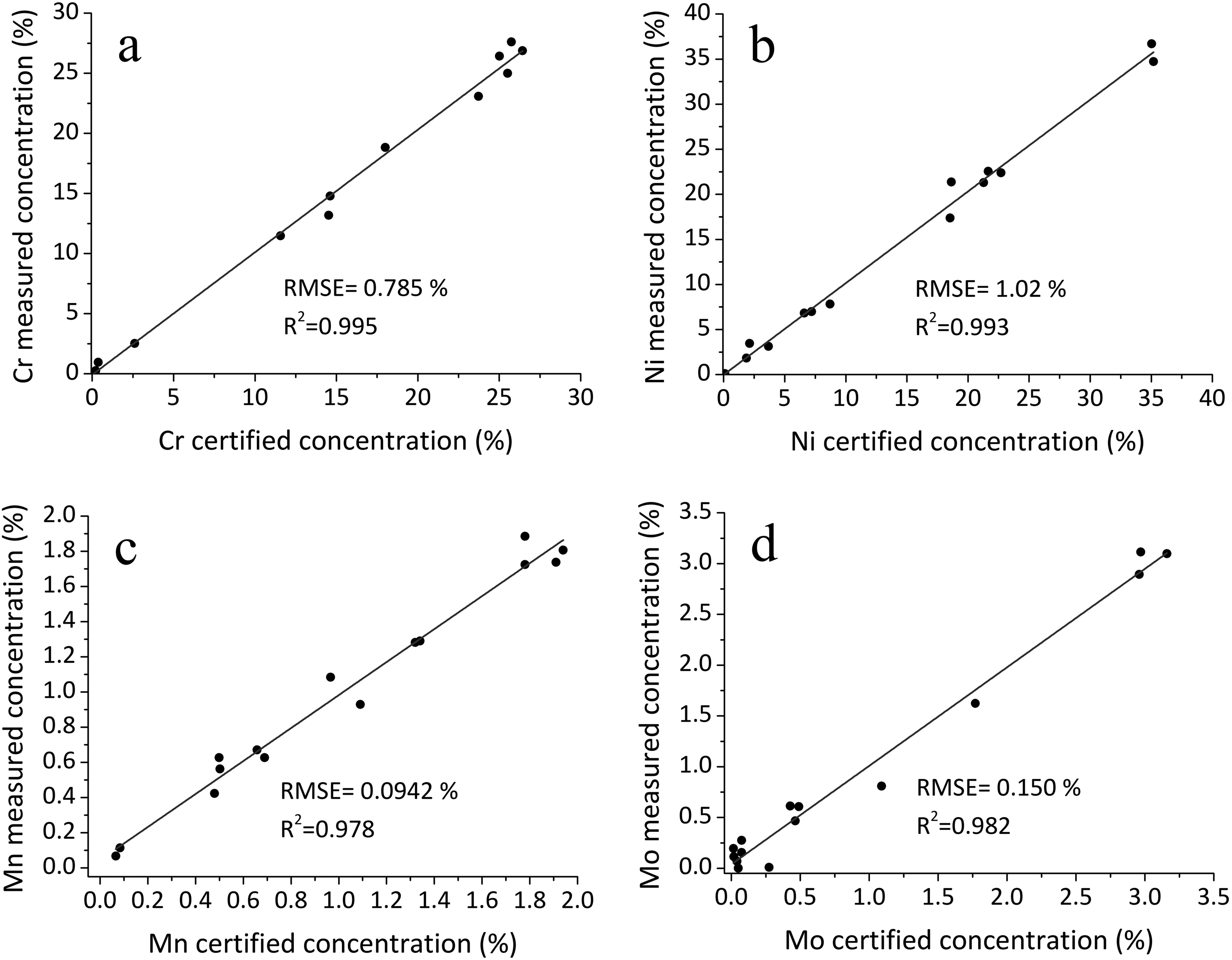
Measured and certified concentration values for the test set: (a) chromium, (b) nickel, (c) manganese, and (d) molybdenum.
Figure 4 illustrates the dependence of the root mean square error (RMSE) on the number of parameters used in the multiparametric calibration model, evaluated by cross-validation (black bars) and on an independent test set (grey bars).
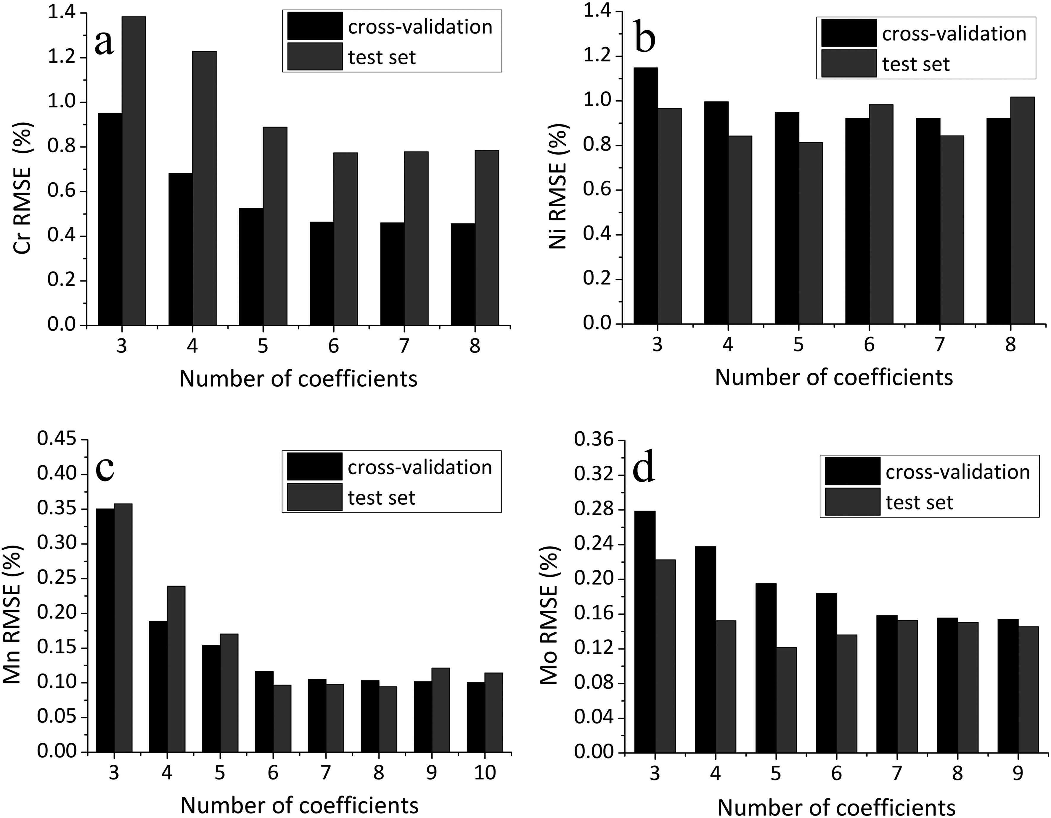
Dependence of RMSE in cross-validation and on the test set for different numbers of parameters for (a) chromium, (b) nickel, (c) manganese, and (d) molybdenum.
For both chromium (Figure 4a) and nickel (Figure 4b), the minimum RMSE during cross-validation was achieved when using eight parameters, indicating an optimal model complexity at this level in terms of training performance. For manganese and molybdenum (Figures 4c and 4d), the lowest cross-validation RMSE was observed for ten and nine parameters, respectively.
However, it is noteworthy that the minimum RMSE on the test set tends to occur at slightly lower model complexities, particularly for chromium and manganese. This discrepancy may reflect overfitting tendencies when too many parameters are included. Nevertheless, in the range of six to eight variables, the RMSE on the test set remains relatively stable, with only modest variations observed. This indicates that the model’s predictive performance is not overly sensitive to minor changes in the number of parameters within this interval.
Thus, the initially chosen upper limit of eight parameters appears to be adequate, though slightly excessive rather than insufficient. The relatively flat RMSE profile on the test set in the range of six to eight variables suggests that a smaller number of parameters may suffice without a significant loss in predictive performance. Nevertheless, the use of eight parameters does not lead to overfitting and ensures stable model behavior across different elements.
Figure 5 shows the effect of excluding outlier spectra-defined based on the intensity of the Fe line-on the accuracy of elemental quantification using LIBS.
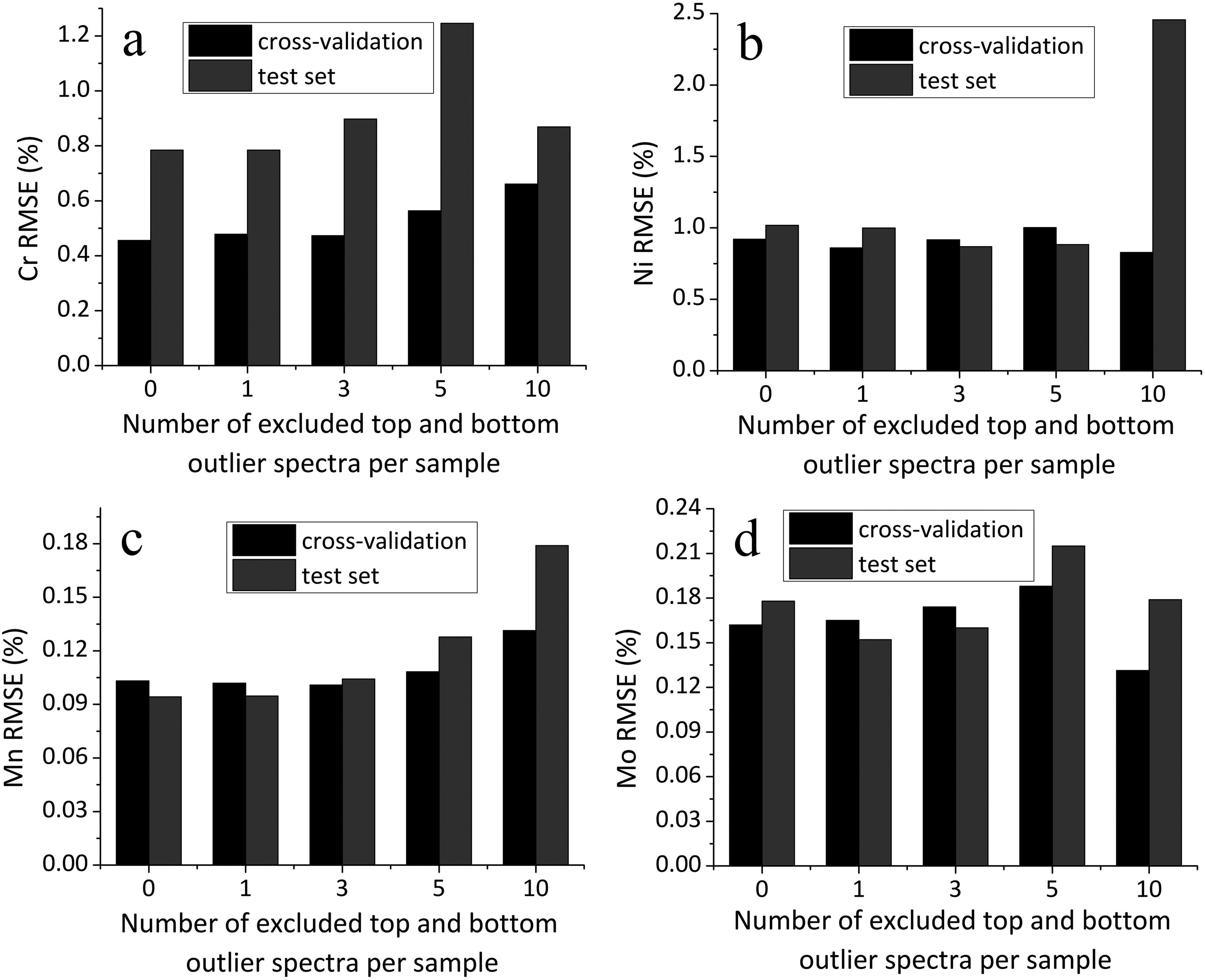
Dependence of RMSE in cross-validation and on the test set on the removal of a varying number of extreme spectra (outliers in iron line intensity) for each sample: (a) chromium, (b) nickel, (c) manganese, and (d) molybdenum.
Although the variation in line intensities across individual spectra collected from the same sample can range widely, from two-fold to as much as 19-fold, the removal of spectra with anomalously high and low Fe line intensity does not lead to any systematic improvement in analytical accuracy. As the number of excluded spectra increases, the RMSE demonstrates a rather fluctuating trend, with no consistent decrease and, in some cases, a slight tendency toward degradation of performance. This suggests that such spectra may still carry meaningful analytical information and that their exclusion does not necessarily enhance, and may sometimes slightly impair, the overall predictive quality of the model.
This behavior can be attributed to the inherently localized nature of LIBS. Each laser pulse probes only a microscale region of the sample, and physical or compositional inhomogeneities, especially in heterogeneous materials such as high-alloy steels, can lead to substantial point-to-point variability. Consequently, averaging over a large number of sampling points is essential to obtain representative results. Excluding outliers based solely on intensity criteria may inadvertently discard physically meaningful information, particularly when such outliers correspond to real variations in local phase composition.
Figure 6 illustrates the effect of dividing the full spectral dataset of each sample into an increasing number of subsets on the prediction accuracy, as quantified by the RMSE in both cross-validation and external test evaluation. While partitioning into two or five subsets does not result in a consistent improvement, with some elements showing slight gains and others experiencing degradation, this variation appears largely unsystematic and likely attributable to random fluctuations rather than robust model enhancement. Notably, splitting into ten subsets leads to a marked increase in RMSE for all elements considered, indicating a clear decline in model performance.
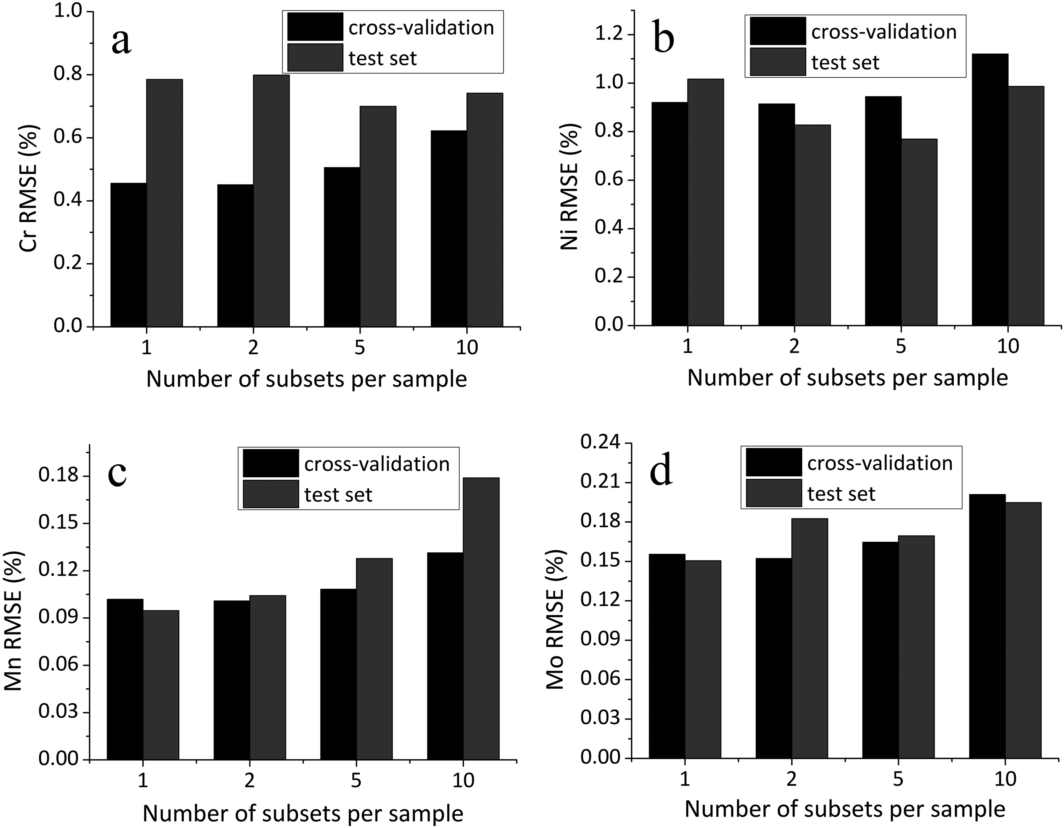
Dependence of RMSE in cross-validation and on the test set on splitting the spectrum set for each sample into a varying number of subsets: (a) chromium, (b) nickel, (c) manganese, and (d) molybdenum.
This degradation may be attributed to a shift in the balance between the quality and quantity of training data. When spectra are averaged over a larger subset (i.e., fewer splits), the resulting input data are less noisy and more representative, leading to better generalization. Conversely, excessive splitting reduces the benefit of signal averaging, increasing the influence of noise and potentially introducing artifacts due to spectral variability within a single sample. It is likely that, given the relatively limited amount of input data necessary for model construction in comparison to the data employed in Képeš et al., 1 the trade-off between data quantity and quality shifts in favor of a smaller number of higher-quality samples. This effect may result from the enhanced signal stability and reduced noise achieved through averaging over fewer but more representative spectra.
The residual plots shown in Figures 2–3 demonstrate an approximately uniform dispersion of prediction errors over the full concentration range, suggesting the absence of pronounced heteroscedasticity. This observation was statistically verified using the Breusch–Pagan test. The obtained p-values were 0.051 (Cr), 0.062 (Mn), 0.317 (Mo), and 0.337 (Ni), all exceeding the significance level α = 0.05, confirming that the null hypothesis of constant error variance cannot be rejected.
Given the verified homoscedasticity, a single residual standard deviation σ, calculated over the entire dataset, serves as an estimator of predictive uncertainty within the compositional domain of the calibration samples. The standard predictive uncertainty can be estimated as σ (RMSE, Table II). The expanded uncertainty (95% confidence level, k = 2) can be estimated as 2σ.
An operational estimate of the limit of detection (LOD) can be expressed as 3σ; however, since no explicit blank signal or local calibration slope is defined in the multivariate model, this value should not be interpreted as a formal International Union of Pure and Applied Chemistry (IUPAC) LOD. Instead, it represents a model-based detection capability within the calibration domain, specifically the minimum concentration variation that can be reliably distinguished from prediction noise within the compositional space covered by the dataset.
These values represent statistical estimates valid within the matrix variability spanned by the calibration dataset and should not be interpreted as universal composition-independent constants. Precision is further evaluated through LOOCV and prediction on an independent validation set. The close agreement between RMSE of cross-validation and RMSE on test set (Table II) indicates consistent predictive performance and suggests that the reported accuracy metrics are not artifacts of internal resampling.
Model structure and the number of calibration parameters are summarized in Figure 4, demonstrating that prediction errors are not associated with excessive model complexity.
Given the multidimensional nature of alloy composition and the limited number of samples (n = 41), the proposed calibration should be interpreted as valid within the compositional region represented by the dataset; extrapolation beyond this domain is not assumed.
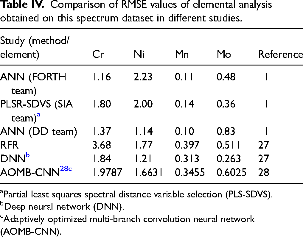
Table IV summarizes previously published results, showing the RMSE values of elemental analysis obtained on the same dataset. For each study, the applied method and the analyzed element are indicated. The results show notable differences in model performance depending on the regression approach and the elemental characteristics.
Comparison of RMSE values of elemental analysis obtained on this spectrum dataset in different studies.
Partial least squares spectral distance variable selection (PLS-SDVS).
Deep neural network (DNN).
Adaptively optimized multi-branch convolution neural network (AOMB-CNN).
The NN model 27 outperformed the random forest regression (RFR) when trained on the subset of spectra selected using the isolation forest algorithm (IFA). This improvement may be attributed to the NN’s ability to capture weak nonlinear dependencies that remain after the removal of spectral outliers, whereas RF tends to approximate the response with piecewise constant regions and may underfit subtle intensity variations.
Notably, the spectral variables identified by the IFA 27 as the most important are located predominantly in the same region of the spectrum, i.e., Mo(II) 281.6 nm, Ni(II) 231.6 nm, Ni(II) 239.4 nm, Cr(II) 285–287 nm, Cr(II) 313 nm, and Cr(II) 336 nm, and partially overlap with those selected in our empirical LIBS-based analysis (Table I), namely, ionic or highly excited atomic lines in the short-wavelength ultraviolet region. These lines are likely associated with the hotter and more stable early phase of the plasma, whereas low-excitation neutral lines may originate from cooler and less stable regions during plasma decay, leading to greater signal variability and reabsorption effects.
The DD team 1 demonstrated notably strong performance for chromium, nickel, and manganese by training a three-layer fully connected NN on a broad spectral range (340–504 nm, 8190 variables) without applying any normalization, filtering, or baseline correction. To mitigate overfitting, data augmentation was performed through random intensity perturbations in the range of ±35% and masking of random spectral segments.
Although this approach requires substantial computational resources, the inclusion of intensity-perturbed spectra likely enabled the network to implicitly learn an effective normalization of the input data.
A potentially more efficient strategy could involve restricting the spectral range to regions surrounding the characteristic lines, as adopted by the FORTH team. 1 Based on the findings of our study, it can also be inferred that the performance of the FORTH team’s NN could have been further improved if the training data had included not only the spectral regions of the four target elements but also those corresponding to other elements present in the samples.
The observed differences in model 1 performances for molybdenum can be explained by the fundamental distinction between PLS regression and neural networks. PLS constructs latent variables as linear combinations of all predictors, explicitly maximizing their covariance with the target variable and therefore retaining sensitivity to weak yet consistent spectral features, even in the presence of strong background variability. In contrast, fully connected neural networks trained on unnormalized spectra tend to suppress low-intensity signals dominated by large-amplitude channels and, given the limited number of training samples typical for LIBS datasets, often fail to capture such subtle correlations reliably. As a result, the PLSR approach employed by the SIA team 1 performed particularly well for Mo, where the main challenge lies in detecting weak spectral lines and mitigating spectral interference from other elements. However, for Cr and Ni, whose spectra are characterized by high intensity and extensive line multiplicity, the linear nature of PLSR likely limited its ability to model complex dependencies.
Another study based on the same dataset 29 investigated the performance of various regression algorithms, including linear, ridge, lasso, decision tree (DT), RFR, and NN, in combination with different dimensionality reduction and feature selection methods such as SelectKBest, principal component analysis (PCA), meta transformer, linear discriminant analysis (LDA), variable importance in projection (VIP) scores from PLS, and recursive feature elimination (RFE). Among the evaluated approaches, the LDA-based dimensionality reduction method yielded the highest accuracy across all regression types. The RFR model achieved the best performance on the all types of dimensionally reduced data, whereas the NN demonstrated superior accuracy when applied to the full-spectrum dataset. However, study 29 reported only the mean squared error (MSE) and the coefficient of determination (R2) for the model as a whole, without providing RMSE values for individual elements, which complicates direct comparison with other works.
The proposed fractional–rational calibration approach occupies an intermediate position between classical linear multivariate methods and fully data-driven machine learning models. In contrast to PLS-type regressions, the rational form explicitly accounts for nonlinear inter-element effects while preserving interpretability of spectral contributions. At the same time, unlike neural network or ensemble approaches, it remains computationally simple and does not require high-dimensional spectral input or large calibration datasets.
Compared to calibration-free LIBS strategies, the method does not rely on plasma diagnostics or thermodynamic assumptions but compensates matrix effects empirically through structured normalization in the denominator. The approach is valid within the compositional domain covered by the calibration samples and should not be extrapolated beyond this region. Given the limited number of samples and selected spectral lines, further validation on independent alloy systems would be required to assess transferability under different experimental conditions.
Conclusion
A new calibration methodology for quantitative LIBS analysis of alloy steels was developed, based on rational multiparametric functions that incorporate spectral line intensities in both the numerator and the denominator. This formulation explicitly accounts for inter-element effects and allows flexible modeling of nonlinear spectral behavior. Compared with classical univariate calibration, the proposed approach provided a consistent reduction in RMSE (Table II), achieving up to a fivefold improvement for elements such as chromium and manganese.
The model’s accuracy and generalizability were further validated on the test set Figure 3, showing low deviation from the certified values and achieving accuracy comparable to the best results reported for this spectrum dataset in the LIBS 2022 regression contest. 1 This underscores the benefit of incorporating a priori knowledge of line positions and their analytical relevance. Overall, despite a number of caveats, the proposed approach offers a more transparent and interpretable alternative to purely statistical models such as PLS, NN, and RFR.
As the current implementation relies on a single spectral line for each element, the method may exhibit reduced stability and increased sensitivity to signal variations, including those arising from spectral interpolation and wavelength shifts. Future work may thus extend this concept toward a NN architecture trained on multiple spectral lines or wavelength regions, in which two dedicated branches learn to represent the numerator and denominator components and are subsequently merged via a division layer. In addition, the results indicate that the optimal spectral subset for NN training should include regions not only with the lines of the target analytes but also with all other alloying elements, which contributes to a more accurate correction for matrix effects.
Footnotes
Acknowledgments
The authors express their gratitude to the team of Képeš et al. 1 for providing access to the dataset.
Consent for Publication
Not applicable.
CRediT Author Statement
None.
Funding
This work was supported by the State Scientific Research Programme “Photonics and Microelectronics 2026–2030” (Task No. 5.1.04).
Declaration of Conflicting Interests
The author(s) declared no potential conflicts of interest with respect to the research, authorship, and/or publication of this article.
