Moving From the Neighborhood to the Cellblock

Abstract

This study examines how prior neighborhood characteristics affect youth’s offending when youths move into an incarceration context. Neighborhood ethnic heterogeneity, residential stability, and disadvantage are often predictive of neighborhood crime, but it is unclear how these neighborhood constructs continue to affect youth’s behavior inside a secure facility. In a sample of recently incarcerated juvenile offenders (N = 320), this study examined how prior neighborhood characteristics affect institutional offending over the first 8 weeks of incarceration. Although disadvantage did not relate to institutional offending, results indicate that youths from racially/ethnically homogenous communities are more likely to offend during the initial weeks of incarceration, whereas youths from residentially stable communities are more likely to offend in the latter weeks.

Keywords

residential mobility ethnic heterogeneity neighborhood incarcerated juveniles

Research and theory on incarceration suggests offenders’ pre-prison socialization affects their behavior and attitudes while incarcerated, and prison behavior is most affected by past experiences (Irwin & Cressey, 1962). While neighborhood and adolescent offending literature suggests that ethnic heterogeneity, residential instability, and disadvantage are important factors for explaining offending in neighborhoods (for reviews, see Leventhal & Brooks-Gunn, 2000; Sampson, Morenoff, & Gannon-Rowley, 2002), there is a dearth of research exploring how offenders’ prior neighborhood characteristics affect their offending behaviors in an incarceration context. This study brings together these two literatures to longitudinally examine how neighborhood factors might matter for understanding juvenile offending during youth’s initial adjustment to a secure incarceration setting.

Incarcerated Juveniles

Research on incarcerated youth stems from decades of theory on adult inmates with most studies focusing on deprivation theory, importation theory, or an integration of both theoretical perspectives. Briefly, deprivation theory posits that the pains of the prison environment through restricted autonomy and the physical characteristics of the incarceration setting lead to inmate offending (Sykes, 1958). On the other hand, importation theory suggests that violence in prison arises from pre-prison attitudes, behaviors, and experiences. Importation theory suggests that the factors predictive of crime outside of prison also predict crime inside prison (Irwin & Cressey, 1962). For example, recent work by DeLisi et al. (2010) suggest that having a high frequency of traumatic events before incarceration leads to higher rates of suicide, sexual misconduct, and total offending while incarcerated. Assuming that adult theories of incarceration apply to juveniles, empirical tests of importation theory on incarcerated youth mostly use individual factors, such as offending history, family structure, race, sex, drug involvement, trauma experiences, and gangs for predicting institutional misconduct (Cao, Zhao, & Van Dine, 1997; DeLisi et al., 2010; MacDonald, 1999; Poole & Regoli, 1983; Trulson, 2007).

One limitation to this research is that there is little understanding of how the characteristics that are imported into prison change over time. Most research on this topic uses cross-sectional data or focuses on a much longer time frame, such as years, that may miss important characteristics as individuals are exposed to the facility. Essentially, the initial incarceration experience is likely different from someone who has been incarcerated for much longer time periods. For example, Brown and Ireland (2006) found that among incarcerated males aged 16 to 20 years, anxiety and depression decreased over time—a finding consistent with research in adult prisoner populations suggesting that the initial period of incarceration is the most stressful (MacKenzie & Goodstein, 1985; Wormith, 1984). The present study highlights this important time period by using data from the first 8 weeks of incarceration. Specifically, the data for this study are from juvenile offenders who are early in their criminal careers and have little or no experience with an incarceration setting. In addition, the initial transition from the neighborhood to the facility is particularly important for this group, as this is a nonnormative experience during a crucial developmental time point.

Neighborhoods and Juvenile Offending

Research on criminal behavior within neighborhoods emanates from Shaw and McKay’s (1942) original social disorganization theory. Extensive research on social disorganization suggests that neighborhood structural characteristics such as ethnic heterogeneity, residential stability, and disadvantage are related to criminal activity within neighborhoods (Bursik, 1988; Bursik & Grasmick, 1993; Sampson & Groves, 1989). Most research supports the notion that higher levels of neighborhood ethnic heterogeneity and diversity are associated with more criminal activity (Hipp, Tita, & Boggess, 2009; Krivo & Peterson, 1996; Rountree & Warner, 1999). Residential stability is expected to create more interactions among residents allowing for more social control and thus reducing crime (Sampson & Groves, 1989; Shaw & Mckay, 1942; cf. Schuck & Widom, 2005; Warner & Pierce, 1993). Neighborhood research on disadvantage and poverty suggests that it increases youth offending (Bursik & Grasmick, 1993; Elliott et al., 1996; Schuck & Widom, 2005), yet some researchers failed to find a significant relation between poverty and crime (Rountree & Warner, 1999).

Although research has shown that neighborhoods are important predictors of criminal activity (Sampson et al., 2002), limited work explores how prior neighborhood characteristics relate to offending behavior once an individual has moved to a new context (for an exception, see Ludwig et al., 2008). For example, high-risk youths move frequently between neighborhoods (Kling, Liebman, & Katz 2007; Sampson & Sharkey, 2008) and often commit crimes outside of their local neighborhood (Morenoff, Sampson, & Raudenbush, 2001; Tita & Griffiths, 2005). Similarly, most research identifies where an offender currently lives to explain why they committed crimes inside and outside of their local neighborhood. This approach suggests that the effects of context can transcend into new environments.

Recent research from the Moving to Opportunity (MTO) housing experiment has provided some insight into the relation between changes in neighborhood context and individual offending (Ludwig et al., 2008). The MTO policy experiment randomly assigned housing vouchers to treatment (received housing voucher) and control (no voucher) groups to test whether a change in neighborhood provided better outcomes (e.g., crime reductions and economic conditions) for disadvantaged families across multiple cities over time (for a review, see Kling et al., 2007). An initial study from the first 2 years of the MTO data suggests that a change from a high poverty neighborhood to a lower poverty area significantly reduces violent juvenile offending (Ludwig, Duncan, & Hirschfield, 2001). However, in a 4-year follow-up study by Kling, Ludwig, and Katz (2005), results indicate that when youths move from a high poverty to a low poverty neighborhood they have significant initial reductions in violent and property offending, but not for violent offending in subsequent years. Results also suggest that property crime for the experimental group significantly increased in later years. Accordingly, the findings from the MTO experiment are mixed (DeLuca & Dayton, 2009) with the specific mechanisms largely unexamined for why this change in offending behaviors occurs in the new context (Ludwig et al., 2001).

Whereas MTO studied how people moved from relatively the same type of neighborhood into varying neighborhoods across a city, our study examines how individuals coming from various neighborhoods affect behavior within a single context. Although MTO studied the effects of relocating youths and their families to neighborhoods that are expected to have less criminal activity, there has been to our knowledge no research conducted on relocating from one’s neighborhood into an incarceration setting. As such, this study builds on this previous work by examining how neighborhood effects impact youth’s offending when they are incarcerated.

Few studies have incorporated neighborhood characteristics as factors that can contribute to offending in incarceration settings. Studies on incarcerated youth have incorporated control variables for youth’s neighborhoods when examining institutional offending, but conceptualizations of neighborhood effects from youth residences before incarceration have been quite limited. For example, MacKenzie (1987) indicates that youth inmates are more likely to be from urban areas. However, Cao et al. (1997) do not find a significant urban effect on incarcerated youth offending when operationalizing their urban effect by using a dichotomous variable to indicate whether the youth committed a crime in a predominately urban county. This lack of finding might be attributed to contextual effects being more micro than the county level, and tests with smaller units of neighborhood aggregations (e.g., tracts and block groups) remain unexamined when studying offending behaviors of incarcerated youths. In addition, prior research on incarcerated adults and juveniles has shown null effects for the impact of family poverty and neighborhood disadvantage on institutional misconduct and violent offending (Harer & Steffensmeier, 1996; Trulson, 2007). To our knowledge, no studies have incorporated other neighborhood factors, such as ethnic heterogeneity and residential stability, as potential correlates for explaining offending behaviors of incarcerated youths.

Goals of the Present Study

Drawing from the neighborhood and crime literature, we suggest that neighborhoods are an important component for understanding youth’s initial experience in an incarceration setting. This study brings together these two literatures to examine how neighborhood factors might matter for understanding offending behaviors within a secure facility. Given the prominence of ethnic heterogeneity, residential stability, and disadvantage in neighborhood research, we use these three constructs as our primary focus. Moreover, importation theory (Irwin & Cressey, 1962) and the prior research on moving (e.g., see Ludwig et al., 2008) suggest the importance of analyzing how prior neighborhood characteristics might relate to institutional offending over time.

This study expands the literature in several ways. First, we use data prospective design. Specifically, we use longitudinal data from the first 8 weeks of incarceration. Given the critical importance of this initial adjustment period to the facility, this study provides insight into the initial window where youths are the most vulnerable. Furthermore, this time frame provides a unique approach to study the transition from the neighborhood to the prison. Second, evidence from the MTO project is mixed with research only focusing on where youths are going and accordingly ignoring from where they are coming from. This study will help shed light on how neighborhoods not only affect behavior once individuals are outside of the local neighborhood but also more specifically within a secure incarceration setting. Third, as outlined in more detail below, this study uses a unique conceptualization of neighborhoods by using census tracts and block groups within the same model. Finally, even though neighborhood research has long argued for the importance of ethnic heterogeneity and residential instability for understating crime, we are not aware of any research that has used prior neighborhood ethnic heterogeneity and residential stability as factors that can contribute to offending in an incarceration setting.

Data

Sample

Participants were 373 males between 14 and 17 years old (M = 16.40, SD = .80) incarcerated in a secure intake facility of the Division of Juvenile Justice (DJJ) in Southern California. The sample was predominantly ethnic minority (53% Latino, 29% African American, 6% White, and 12% Other, with other being mainly multiracial), which is representative of incarcerated youths in similar facilities in California (California Department of Justice, 2002). Youth varied in their commitment offenses, but primarily comprised serious offenders with 70% being convicted of a person offense, such as robbery (25%), aggravated assault (17%), sexual assault (5%), and murder (3%). After person offenses, youth were most likely to be incarcerated for property crimes (e.g., burglary, auto theft, receiving stolen property; 12%), public order (7%), weapon offense (3%), drug offense (4%), or other offenses (e.g., status offenses, violation of probation; 4%).

The present sample was limited to youths with complete interview data and with a geocodable address prior to incarceration (obtained from institutional records). Youths without complete interview data (n = 35) or without an address from facility records (n = 12) were similar to the final sample demographically (race and age). Of the 361 youths with an address, 334 (93%) were successfully geocoded in ArcGIS Version 9.3 (see Geocoding section for the procedure). Addresses that could not be geocoded in ArcGIS (n = 27) were then geocoded in Google Earth Pro (successful n = 21).¹ Of the youths with addresses, 6 were not geocoded. Thus, youths without complete interview data, without an address, or an address that was not geocoded were necessarily excluded from the present study. The final analytical sample consisted of 320 youth.

Data Collection and Procedure

The DJJ facility was contacted daily to determine any new arrivals, and all youth who were admitted into the facility on a new charge were eligible for enrollment within 48 hr of their arrival. Over the course of 2 years (Spring 2005-Spring 2007), participants were approached about the nature of the study (verbally and in writing). Written assent was obtained from all youth and verbal consent was acquired from the parent/guardian via a tape-recorded telephone conversation (97% of the parents contacted allowed their child to participate in the study). A Certificate of Confidentiality from the Department of Health and Human Services was obtained to ensure participants’ confidentiality and the Institutional Review Board at the University of California, Irvine, and the California Department of Corrections and Rehabilitation approved all study procedures.

Each youth participated in a 2-hr structured baseline interview. After the baseline interview, youths were interviewed weekly for the next 3 weeks during their first month in the facility and also 4 weeks later during their second month in the facility (5 total interviews over an 8-week period). The follow-up interviews lasted approximately 1.5 hr. Each participant was given a copy of the interview, while research assistants read questions aloud, recorded responses, and provided clarification when necessary. In addition, official institutional records (home address, infractions and disciplinary actions, commitment offense, etc.) were collected from the facility as case reports for each participant.

Institutional Offending—Dependent Variables

The dependent variable for this study—institutional offending—was calculated based on data obtained from institutional records. Like all official data, it suffers from not all incidents being reported or recorded (e.g., see Daggett & Camp, 2009). However, we have no reason to believe these reports are any less valid than other juvenile incarceration studies using official data (e.g., see DeLisi et al., 2010; MacDonald, 1999; Trulson, 2007). All infractions deemed as minor (e.g., inappropriate dress, grooming/hygiene standards) by the institution were excluded in the analyses, and models were estimated for nonviolent and violent offending. Violent offenses involved physical attacks or altercations regardless of injuries (e.g., assault on staff with or without a weapon, assault on a youth with a weapon or a vile substance, physical altercation that requires the use of chemical and/or physical restraints to stop the altercation). For violent offending, 48% of the youth had no violent offenses across the 8 weeks, 31% had one violent offense, and 11% had more than two violent offenses. Nonviolent offending involved verbal or written threats, harassment, abuse of staff, wards, or persons not in custody; damaging, defacing, or destroying property; possession of any controlled substance, drug, or alcohol; and possession, control, or manufacture of a weapon, explosive device, or other object. For nonviolent offending, 45% had no offenses across all 8 weeks, 23% had one nonviolent offense, 27% had between two and five offenses, and 5% had more than six offenses. Institutional offending data were aggregated at the weekly level as the number of infractions per week (frequency) for the first 8 weeks of incarceration.

Neighborhood Measures—Independent Variables

Geocoding

Using a Geographic Information System (GIS), youths’ addresses from facility records were geocoded to give each address an exact latitude and longitude location. Before geocoding, Google Maps was used to clean addresses and ensure an accurate geocode (e.g., 1308 Friendship would be cleaned to 1308 Friendship Road). Youths’ addresses were geocoded to streets from the 2008 Environmental Systems Research Institute’s (ESRI) StreetMap USA (Redlands, California) and Google Earth Pro. We used a minimum match (how closely the youth’s address matched the address from the reference data) score of 70, a spelling sensitivity score of 70, and applied an end offset of 25 feet to move the point away from the street centerline (Drummond, 1995).² As this study recruits participants from a DJJ intake center, youths were from all over Southern California with the majority from Los Angeles County (43%).

Defining a Neighborhood

Although most neighborhood studies only focus on one geographic unit for defining a neighborhood (e.g., Census tracts), this approach assumes that neighborhood processes (e.g., residential stability, ethnic heterogeneity, and disadvantage) operate similarly across different levels of aggregation.³ This approach is modeled after the work by Hipp (2007) who has shown that the level of aggregation can provide differences in the effects of neighborhood characteristics on crime rates and further suggests that the level of neighborhood aggregation should reflect the theoretical construct of interest.⁴ As such, this study uses different neighborhood aggregations depending on how the social process of interest theoretically operates. For ethnic heterogeneity, we use tracts because larger units of aggregation are suggested to have a greater impact on perceptions of crime (Hipp, 2007). For residential stability, block groups are used to represent neighborhoods given that residential stability at smaller units of aggregation fosters a stronger sense of community cohesion that in turn exerts stronger control over residents (Hipp, 2010). Consistent with much prior work, tracts are used to represent neighborhood disadvantage (Jargowsky, 1997; Wilson, 1990).⁵ Based on the latitude and longitude location from geocoding, addresses were linked to 2000 Census information from GeoLytics by spatially joining the latitude and longitude points to neighborhood polygons (census tracts and block groups).

Ethnic Heterogeneity

To operationalize the ethnic heterogeneity in the neighborhood, a Herfindahl index was used (Gibbs & Martin, 1962) to measure the structure of the neighborhood racial composition using five racial groups (Black, White, Latino, Asian and Pacific Islander, and Other [Native American, Multiracial, and Other]). This measure ranges on a scale from 0 being perfectly homogenous (one race is 100% of the neighborhood) to .80 being all races are equally distributed in a neighborhood (heterogeneous).

Residential Stability and Disadvantage

Given that many neighborhood variables are theoretically related to the same construct (e.g., poverty and unemployment for disadvantage), a principal components factor analysis was used to operationalize disadvantage and residential stability. The stability and disadvantage factors are derived from Sampson, Raudenbush, and Earls’ (1997) work that examines neighborhood effects. However, the percent Black is not included in the principal components analysis as a part of the disadvantage factor because it is unlikely that only one race is disadvantaged (Peterson & Krivo, 2005), especially in southern California where there is a large population of Latinos. The stability construct is the proportion of residents who own their home out of all occupied housing units, and the proportion of residents who stayed in the same home since 1995 out of all residents who are aged 5 years or older. For the disadvantage construct, we use the proportion unemployed, proportion on public assistance, proportion poverty, and proportion single-parent households (see Table 1, for the summary statistics of the neighborhood variables).

Table 1.

Summary Statistics of Neighborhood Variables.

Variables	M	SD	Minimum	Maximum
Proportion public assistance	0.103	0.087	0.000	0.491
Proportion poverty	0.235	0.145	0.011	0.695
Proportion unemployed	0.114	0.072	0.000	0.442
Proportion single-parent households	0.208	0.111	0.000	0.618
Proportion residents in same house since 1995	0.482	0.132	0.100	0.827
Proportion homeowners	0.494	0.265	0.000	0.966
Ethnic heterogeneity	0.516	0.154	0.021	0.763

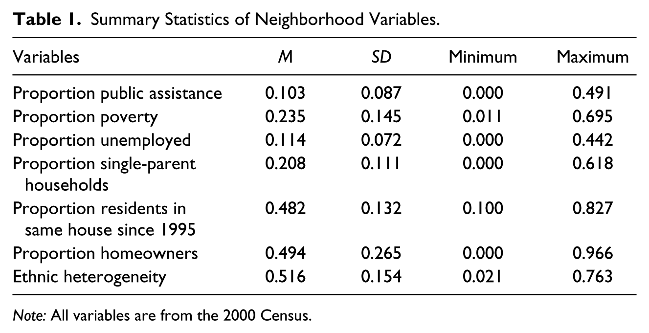
Note: All variables are from the 2000 Census.

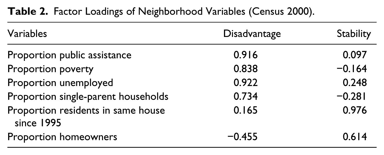
Factor scores were rotated using a promax (oblique) solution that allows for the factors to be correlated and factors with eigenvalues greater than one were used in the analyses (Kaiser, 1960). This technique provided a two-factor solution, disadvantage and stability, with 84% of the variance explained by the two factors (21% for stability and 63% for disadvantage). The stability factor ranged from −2.52 to 2.26 standard deviations and the disadvantage factor ranged from −1.68 to 4.95 standard deviations. The two items for the stability factor are significantly correlated (r = −.28, p < .0001) and the reliability estimate for the disadvantage factor was high (Cronbach’s α = .86). The results of the principal components analysis are presented in Table 2.

Table 2.

Factor Loadings of Neighborhood Variables (Census 2000).

Variables	Disadvantage	Stability
Proportion public assistance	0.916	0.097
Proportion poverty	0.838	−0.164
Proportion unemployed	0.922	0.248
Proportion single-parent households	0.734	−0.281
Proportion residents in same house since 1995	0.165	0.976
Proportion homeowners	−0.455	0.614

Other Independent Variables

Several control variables were of interest for the present analyses: race, age, violent commitment offense, and recommitment to the facility. Race was measured with four dummy variables from each participant’s self-report (Latino as the reference group; see “Data” section for breakdown). Age by year was included in all models (age 14 = 3.12%, 15 = 10.62%, 16 = 29.06%, 17 = 57.19%). A dichotomous commitment offense variable (violent or nonviolent) was calculated based on institutional records. Because this sample is comprised of the most serious juvenile offenders in California, it is not surprising that the majority were committed for a violent offense (70%). To measure recommitment to the facility, participants at baseline were asked, “Have you been to the facility before?” This dichotomous variable was added to the analyses to account for participants who may be more familiar with the secure facility and therefore less affected by the move into the facility environment (5% in the facility before).

Analytical Strategy

Count models in Stata Version 10 were estimated for violent and nonviolent institutional offending to test how neighborhood characteristics from a youth’s residence predict their offending behaviors in a secure juvenile facility over time. As the outcomes (number of offenses) are counts, the dependent variables are not continuous or normally distributed. We used negative binomial regression models that account for the excessive variation between counts.^6,7 As this study uses panel data, and the observations are not independent with the same individuals being measured repeatedly over time, a random effects approach was used to explain the unobserved heterogeneity between observations and time (Gardner, Mulvey, & Shaw, 1995; Osgood 2000).⁸ A more detailed description of the analytical strategy can be found in the appendix.

Models were estimated for violent and nonviolent offending with all variables except time (weeks in the facility) grand mean centered to estimate the effect of the average incarcerated youth’s neighborhood. We tested the functional form of each offending type by including polynomials of time raised to different powers until it was no longer a significant predictor in each model. Neighborhood variables, disadvantage, residential stability, and ethnic heterogeneity, were included in the model as a time invariant predictor as well as an interaction between each neighborhood variable and time. These cross-level interactions are useful for understanding how the effects of a youth’s previous neighborhood change over time during the first 8 weeks of incarceration (i.e., if the effect of neighborhood context on offending become stronger or weaker over time).⁹ In all models, all of the previously mentioned variables were controlled for and tests for multicollinearity and influential observations were conducted.¹⁰

Finally, given the fluidity of the DJJ, some youths were transferred to other facilities between the fourth and eighth week assessments with n = 307 (95.9%) at the end of Week 4 compared with n = 220 (68.7%) at the end of Week 8. Only 11 youths (3%) withdrew voluntarily over the course of the study. To investigate the impact of attrition on our analyses, we developed a selection model in which the outcome was whether the youth left the facility at any point over the entire study. While another approach would be to longitudinally model attrition, we chose to use a cross-sectional approach because it is a more conservative test. We estimated a probit selection model that contained the same measures presented in Table 3 (excluding the interactions). No significant effects for these measures were observed in the selection model (results not shown). This suggests that there are no differences in neighborhood characteristics or demographics when comparing those who left the facility to those who stayed in the facility for the duration of the study. Based on this selection model, we also calculated an inverse Mills ratio (e.g., see Bushway, Johnson, & Slocum, 2007; Heckman, 1976) and estimated models for violent and nonviolent offending without any predictors. The inverse Mills ratio was never significant. When we estimated the full models with all of the variables from Table 3, the models were quite similar when the inverse mills ratio was included or not (it was never significant), but this model had extensive multicollinearity, which is not surprising (e.g., see Stolzenberg & Relles, 1997; Winship & Mare, 1992). To further address this issue, we weighted the data by the inverse mills ratio when estimating the models, and the results were unchanged. Thus, we have no evidence that attrition affected our findings, and present the results without the inverse Mills ratio.

Table 3.

Unstandardized Coefficients for Violent and Nonviolent Offending.

	Violent offending	Nonviolent offending
Variables	Coefficient (SE)	Coefficient (SE)
Intercept	2.490 (2.810)	−2.043 (0.252)***
Time	−0.051 (0.028)****	0.510 (0.109)***
Time squared	—	−0.057 (0.015)***
Ethnic heterogeneity	−0.015 (0.007)*	−0.005 (0.008)
Ethnic heterogeneity × Time	0.003 (0.002)*	0.002 (0.002)
Disadvantage	0.037 (0.117)	0.027 (0.134)
Disadvantage × Time	−0.006 (0.030)	0.012 (0.030)
Residential Stability	−0.138 (0.113)	−0.114 (0.133)
Residential Stability × Week	0.062 (0.029)*	0.072 (0.032)*
Control variables
Latino youth reference group
White (0/1)	−0.470 (0.381)	−0.566 (0.343)****
Black (0/1)	−0.060 (0.185)	−0.021 (0.165)
Other (0/1)	0.244 (0.206)	−0.061 (0.202)
Age	−0.122 (0.087)	−0.124 (0.080)
Violent commitment offense (0/1)	−0.232 (0.153)	−0.319 (0.139)*
Been to facility before (0/1)	0.666 (0.279)*	0.457 (0.261)****
Random effects
Across individuals (logged)	5.454 (2.660)*	2.492 (0.486)***
Dispersion (logged)	0.981 (0.396)*	1.860 (0.611)**
Log likelihood	−844.754	−1037.587
Observations	2,217	2,217
N	320	320

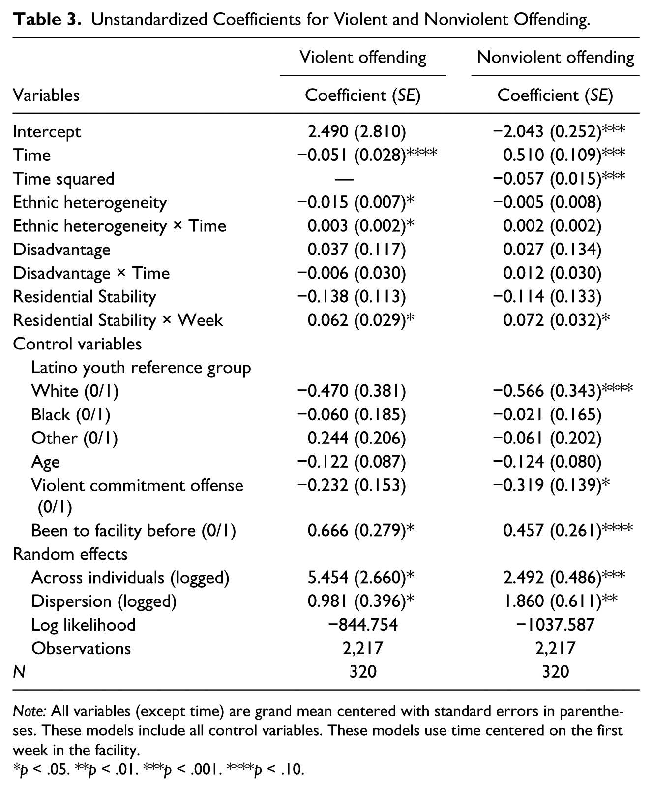
Note: All variables (except time) are grand mean centered with standard errors in parentheses. These models include all control variables. These models use time centered on the first week in the facility.

p < .05. **p < .01. ***p < .001. ****p < .10.

Results

Upon examination of the mean trajectories of institutional offending across the first 8 weeks of incarceration, violent offending was higher than nonviolent offending during the first week only. Interestingly, whereas violent offending remains somewhat steady over time, nonviolent offending increased for the first 6 weeks and then declined thereafter (Figure 1). A linear functional form fit best for violent offending (p < .10), and a quadratic change trajectory was optimal for nonviolent offending (p < .01). As the nonviolent offending model follows a quadratic trajectory, interactions were also tested between the neighborhood variables and a time-squared variable, but these interactions were not significant and accordingly dropped from the analyses.

Figure 1.

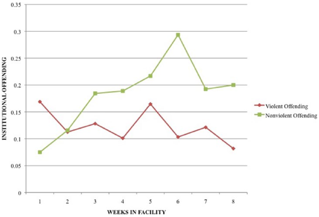
Mean offending behavior (violent and nonviolent) across time in the facility.

We briefly discuss the results of the control variables for violent and nonviolent offending models. No differences were shown in offending between Latino youths and the other races. We also found no difference between the ages of youth for violent or nonviolent offending. This finding is likely due to the lack of variability in the ages of our respondents given that approximately 86% of the youth are between the ages of 16 and 17. Youths who had been to the facility before were more likely to violently offend (p < .05). Finally, youths who had a nonviolent commitment offense were significantly more likely to nonviolently offend inside the facility (p < .05).

Violent Offending

Ethnic Heterogeneity

When predicting violent offending within the facility, neighborhood ethnic heterogeneity was found to have a significant main effect as well as an interactive effect with time (see Table 3). The model in Figure 2 shows that youths from communities with lower ethnic heterogeneity (one standard deviation below the mean) had higher rates of violent offending during the initial 3 weeks at the facility than the average (mean) youth.¹¹ Youths from neighborhoods with lower ethnic heterogeneity had significantly more offending during the first 3 weeks in the facility (p < .05 for Weeks 1-2, p < .1 for Week 3). Specifically, youths from neighborhoods with lower ethnic heterogeneity had 3.1 more violent offenses than the average youth during the first week of incarceration, 2.3 more violent offenses during the second week, and 1.6 more violent offenses in the third week. There were slight differences between low and high ethnic heterogeneity at Week 4, and by the second month, youths from neighborhoods with higher ethnic heterogeneity did not offend at a significantly different rate. In sum, this finding indicates that youths from neighborhoods with lower ethnic heterogeneity (homogeneous communities) have significantly higher rates of offending during their first 3 weeks of incarceration than youths from neighborhoods with higher ethnic heterogeneity (diverse neighborhoods).¹²

Figure 2.

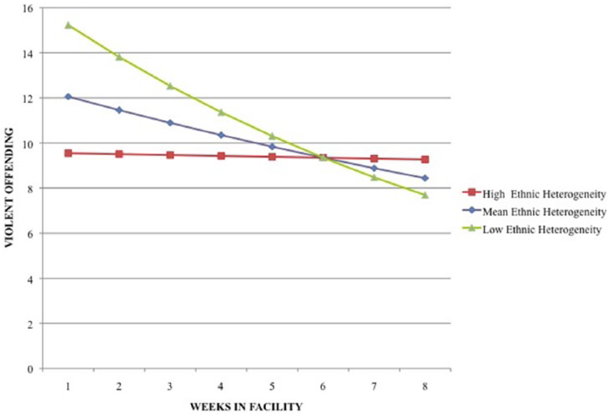
Trajectory of the effect of ethnic heterogeneity on violent offending.

Residential Stability

Although residential stability was not significantly related to offending in the first week, the interaction between residential stability and time suggested that significant differences occur over time for violent offending. Specifically, youths from neighborhoods with higher residential stability slightly increased in their rate of offending across time (see Figure 3). No significant differences were found for the main effect of residential stability on violent offending for Weeks 1 through 5. However, Weeks 6 and 7 were trend associations (p < .10) and Week 8 was significant (p < .05). Youths from neighborhoods with higher residential stability (one standard deviation above the mean) are expected to have 1.7, 2.3, and 2.89 more violent offenses than the average youth for Weeks 6, 7, and 8 respectively.

Figure 3.

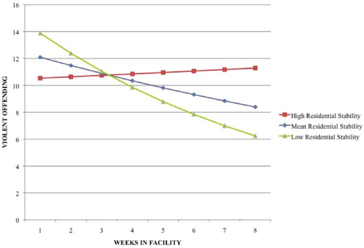
Trajectory of the effect of residential stability on violent offending.

Disadvantage

Although much research has highlighted the importance of neighborhood disadvantage on crime rates (Elliott et al., 1996; Jencks & Mayer, 1990; Krivo & Peterson, 1996; Sampson & Morenoff, 2006), this hypothesis was not supported in the models for violent offending. To further investigate this lack of effect, models were also estimated for both offending types without the control variables and disadvantage was still not significant. Furthermore, models were estimated for violent and nonviolent offending without the controls and other neighborhood predictors and disadvantage was again not significant.

Nonviolent Offending

Ethnic Heterogeneity

Ethnic heterogeneity did not exhibit any main effects or significant interactions with time in the models for nonviolent offending (see Table 3).

Residential Stability

In the analysis examining the effects of residential stability on nonviolent offending (Figure 4), there were only slight differences between youths from neighborhoods low and high on residential stability during the first 4 weeks. In Weeks 5 through 8, youths from neighborhoods with more residential stability had higher rates of nonviolently offending (p < .05 for Week 5, p < .01 for Weeks 6-8) than youths from less residentially stable neighborhoods. Specifically, youths from high stability neighborhoods were found to have .07 more nonviolent offenses than the average youth in the fifth week, .11 more nonviolent offenses in the sixth week, and .13 more nonviolent offenses in the seventh and eighth week.

Figure 4.

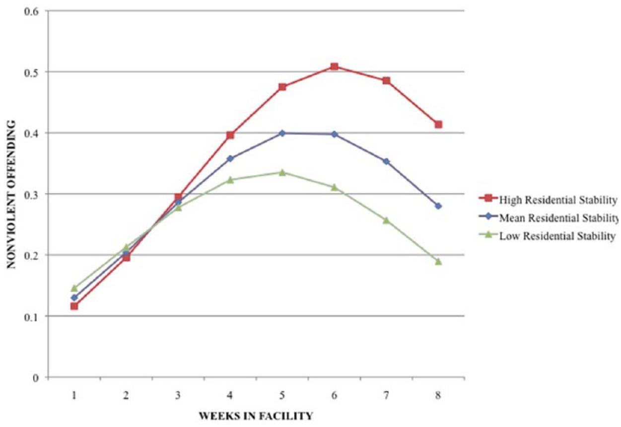
Trajectory of the effect of residential stability on nonviolent offending.

Disadvantage

Similar to the violent offending models, disadvantage did not have a significant main effect or interactive effect with time when predicting nonviolent offending.

Discussion

Decades of theory and research have argued that the local neighborhood’s disadvantage, residential instability, and ethnic heterogeneity are related to increased neighborhood crime. Yet, few studies have actually tested how neighborhood factors operate outside of the urban environment (Osgood & Chambers, 2000) or when residents have moved into a new context (for an exception, see MTO). This study extends this prior research by examining how neighborhoods continue to affect youth’s offending behaviors once they have been incarcerated in a secure facility. Our results suggest that youths from ethnically homogeneous communities are more likely to offend during the initial weeks of incarceration than youths from diverse neighborhoods, whereas youths from residentially stable communities are more likely to offend in latter weeks of incarceration than youths from residentially unstable neighborhoods. These findings suggest that neighborhood factors from a prior context may operate differently when exposed to a new context.

Although moving from one’s neighborhood into an incarceration setting is conceptually different from residential mobility in the streets, our results suggest that youths from stable and homogeneous communities are more likely to violently offend during their initial adjustment to the incarceration context. When youths move from neighborhoods with little ethnic diversity into the incarceration setting, these youths are more likely to offend during their initial few weeks of adjustment in the facility. This result suggests that youths coming from more homogeneous neighborhoods may have a particularly difficult time adjusting to the incarceration setting in the first few weeks. However, as these youths become more accustomed to the incarceration context, they are less likely to exhibit violent offending behaviors. In turn, although much neighborhood research has suggested that increased ethnic heterogeneity leads to higher rates of neighborhood crime (e.g., see Hipp et al., 2009), this study indicates that ethnically heterogeneous neighborhoods may serve a protective function for youth when initially moving into an ethnically diverse incarceration setting. Similarly, Graham’s (2006) research in Los Angeles schools has shown that classrooms with more ethnic diversity have less victimization than classes dominated by a majority race. Perhaps this finding from schools applies to neighborhoods in that a “balance of power” between races may actually reduce offending (Graham, 2006, p. 318). Future research may explore these findings further by examining how different racial/ethnic groups interact or, in this instance, who attacks whom when exploring institutional misconduct. Accordingly, it would be interesting to know whether youths from ethnically homogeneous neighborhoods attack others who are of a similar race/ethnicity or from another racial/ethnic group.

Results from this study also indicate that youths from residentially stable communities are more likely to offend during the second month of incarceration. The neighborhood and crime literature suggests that residentially stable neighborhoods reduce criminal activity because residents are expected to be more cohesive (Morenoff & Sampson, 1997; Shaw & McKay, 1942; Warner & Rountree, 1997). One interpretation of our findings would suggest that the bonds with the outside world (e.g., ties to family and friends) would weaken the longer a youth is incarcerated. As a result, the absence of social support from the local community network (e.g., from family and friends) inside the facility may provoke youth violence (Borgman, 1985). Youths from stable communities may be expected to offend less initially, but might be increasingly likely to offend more as ties are extinguished with the local community across time. Future research might examine how the residential stability of the prison environment via the churning of prisoners affects youth offending.

While this study does find that the previous neighborhood is related to offending behaviors inside a secure incarceration facility, the lack of support for disadvantage is of note. Although much neighborhood research shows an effect for disadvantage (Bursik & Grasmick, 1993), evidence from the adult and youth incarceration literature suggests this is not always the case by showing that disadvantage does not predict violent offending or institutional misconduct (Harer & Steffensmeier, 1996; Trulson, 2007). Recent research from Trulson, DeLisi, Caudill, Belshaw, and Marquart (2010) also finds that while a majority of youth come from families in poverty, they reported no differences in misconduct or assaults when using a dichotomous measure of whether a youth’s family was in poverty. As such, the effects of disadvantage may operate differently when outside of the local neighborhood and does not appear to affect offending when examining differences between incarcerated youth.

One practical implication from our study indicates that knowing where youth resided before entering an incarceration context may help to prevent institutional misconduct. Youths from ethnically homogeneous and residentially stable neighborhoods appear to have a much different incarceration experience than youths from ethnically heterogeneous and residentially unstable neighborhoods. Information about youth’s neighborhoods may provide facility staff with a better understanding of youth misconduct, as well as another source of information to help make more informed housing decisions in the facility.

Most neighborhood studies are cross sectional, but this study is strengthened by longitudinally exploring youths over the initial 8 weeks in a facility. Although some scholars have argued that longitudinal research is unjustified (Gottfredson & Hirschi, 1987), this study emphasizes the need for longitudinal research because different conclusions may have resulted when sampling these youths using cross-sectional analysis. For example, if youths were sampled only at the first month, the results would only suggest an effect for ethnic heterogeneity but not for residential stability. Yet, a sample from the second month would show an effect for residential stability and not ethnic heterogeneity. In addition, while much research has examined the effects of when prisoners return to their communities on parole (e.g., see Clear, 2007, Lattimore, MacDonald, Piquero, Linster, & Visher, 2004), this study examines a unique time period when juveniles are adjusting from their communities to an incarceration facility. Finally, this study uses multiple representations of neighborhoods (e.g., block groups and tracts) in the same model to more effectively gauge how structural neighborhood factors might operate.

Although this study has added to the understanding of the how neighborhoods affect individual delinquency inside an incarceration setting, it has some limitations. First, due to data restrictions, it is unclear how long it has been since youth left their neighborhood. Second, we used a case study approach, and thus we have no variability and no measures of how the facility context might impact offending. Future research might extend our findings by exploring the interaction between the neighborhood and facility context when exploring institutional misconduct. Third, it is difficult to interpret how the findings would generalize to youths moving in the neighborhood as the incarceration setting may moderate the effects of neighborhoods and youths are forced to move into the facility. Accordingly, the results are conditional on youths who are selected into an incarceration setting. Finally, the conceptualization of the neighborhood context is limited to only three characteristics (disadvantage, residential stability, and ethnic heterogeneity). Future research might address this issue by focusing on other factors, such as physical neighborhood disorder (e.g., broken windows) and neighborhood cohesion (e.g., social ties and collective efficacy) to provide a richer estimate of the neighborhood context.

Despite these limitations, this study offers important future directions and challenges for ecological studies of crime and theories on incarcerated juveniles. Future studies exploring the debate between importation and deprivation theories might benefit from taking into account the larger social context prior to incarceration in tandem with individual risk factors. These results suggest that certain neighborhood contexts (e.g., stability and ethnic heterogeneity) predict offending even within an incarceration setting. Thus, knowing where youth come from is critical for understanding their behavior. Whether the effects noted here are maintained, or change, over a longer course of incarceration (months or years) remains an important question for future research. Given that the prior neighborhood context influences offending behaviors while juveniles are incarcerated, it is important for future research to consider how neighborhood characteristics and prior incarceration might operate when these youth return home.

Footnotes

Appendix

We use a random effects modeling strategy because this study focuses on change between individuals, rather than change within individuals as with fixed effects techniques (Cameron & Trivedi, 1998). As such, a fixed effects approach is not an appropriate modeling strategy because it calls for including each individual in the model, and fixed effects are unable to identify the effects of individual time stable variables, such as race (Brame, Bushway, & Paternoster, 1999). The random effects negative binominal regression assumes that the dispersion in the outcome variable varies randomly over time and between people by following a beta distribution (see Hausman, Hall, & Griliches, 1984, for the specific derivation). For this study, the random effects negative binomial model follows a beta distribution because each individual’s level-two intercept is dependent on the level-one intercept (i.e., time in the facility). Accordingly, the random effects are distributed across individuals and are essentially “layered” onto the negative binomial model (Hilbe, 2007, p. 212). By allowing for the dispersion to vary randomly between individuals and time, the random effects negative binomial regression is preferred because it can better account for the heterogeneity in the data across time.

A model for this study can be expressed as follows:

y_{i t} = \exp (β_{0} + β_{1} {time}_{i t} + β_{2} {disadvantage}_{i} + β_{3} {disadvantage}_{i} \times {time}_{i t} + β_{4} {stability}_{i} + β_{5} {stability}_{i} \times {time}_{i t} + β_{6} {heterogeneity}_{i} + β_{7} {heterogeneity}_{i} \times {time}_{i t} + \dots β_{k} X_{i}) + a_{i t} + b_{i t} + ε_{i}

where $y_{i t}$ represents the expected count of offending for individual i in week t, $β_{0}$ is the intercept, $a_{i t}$ is the random component to account for unexplained heterogeneity that changes across individuals and is assumed to be independent of all explanatory variables $X_{i}$ , $b_{i t}$ is the dispersion parameter, and $ε_{i}$ is the random error term across individuals. As counts of offending must be positive, the coefficients can be interpreted as $y_{i t} = \exp (β_{k} X_{i})$ , where a 1-unit increase in $X_{i}$ multiplies the expected offending by a factor of exponentiated ( $β_{k}$ ; Gardner, Mulvey, & Shaw, 1995).

Acknowledgements

We are especially grateful to the many individuals responsible for the data collection and preparation. We also thank John Hipp, George Tita, and the members of the Development, Disorder, and Delinquency lab for reviewing earlier drafts.

Declaration of Conflicting Interests

The author(s) declared no potential conflicts of interest with respect to the research, authorship, and/or publication of this article.

Funding

The author(s) disclosed receipt of the following financial support for the research, authorship, and/or publication of this article: Funding for this study was provided to Elizabeth Cauffman, PhD, from the National Institute of Mental Health (K01MH01791-01A1) and from the Center for Evidence-Based Corrections at the University of California, Irvine.

Notes

Author Biographies

Adam Boessen is a doctoral candidate in the Department of Criminology, Law, and Society at the University of California, Irvine. His primary research interests include the community of context of crime, spatial analysis, social networks, and juvenile delinquency.

Elizabeth Cauffman is a professor in the Department of Psychology and Social Behavior at the University of California, Irvine. Her research involves identifying developmental trajectories of delinquency, developing diagnostics to improve the identification of treatment needs among youthful offenders, and exploring the legal implications of research on the development of mature judgment.

References

Borgman

(1985). The influence of family visiting upon boys’ behavior in a juvenile correctional institution. Child Welfare, 64, 629-638.

Brame

Bushway

Paternoster

(1999). On the use of panel research designs and random effects models to investigate static and dynamic theories of criminal offending. Criminology, 37, 599-642.

Brown

S. L.

Ireland

C. A.

(2006). Coping style and distress in newly incarcerated male adolescents. Journal of Adolescent Health, 38, 656-661.

Bursik

R. J.

(1988). Social disorganization and theories of crime and delinquency: Problems and prospects. Criminology, 26, 519-551.

Bursik

R. J.

Grasmick

H. G.

(1993). Neighborhoods and Crime: The dimensions of effective community control. Boston, MA: Lexington Books.

Bushway

Johnson

B. D.

Slocum

L. A.

(2007). Is the magic still there? The use of the Heckman two-step correction for selection bias in criminology. Journal of Quantitative Criminology, 23, 151-178.

California Department of Justice. (2002). Juvenile justice in California 2002. Sacramento, CA: Division of California Justice Information Services.

Cameron

A. C.

Trivedi

P. K.

(1998). Regression analysis of count data. New York, NY: Cambridge University Press.

Cao

Zhao

Van Dine

(1997). Prison disciplinary tickets: A test of the deprivation and importation models. Journal of Criminal Justice, 25, 103-113.

10.

Clear

T. R.

(2007). Imprisoning communities: How mass incarceration makes disadvantaged neighborhoods worse. New York, NY: Oxford University Press.

11.

Daggett

D. M.

Camp

S. D.

(2009). Do official misconduct data tell the same story as the individuals who live in prison? Criminal Justice Review, 34, 428-449.

12.

DeLisi

Drury

A. J.

Kosloski

A. E.

Caudill

J. W.

Conis

P. J.

Anderson

C. A.

Beaver

K. M.

(2010). The cycle of violence behind bars: Traumatization and institutional misconduct among juvenile delinquents in confinement. Youth Violence and Juvenile Justice, 8, 107-112.

13.

DeLuca

Dayton

(2009). Switching social contexts: The effects of housing mobility and school choice programs on youth outcomes. Annual Review of Sociology, 35, 457-491.

14.

Drummond

W. J.

(1995). Address matching: GIS technology for mapping human activity patterns. Journal of the American Planning Association, 61, 240-251.

15.

Elliott

D. S.

Wilson

W. J.

Huizinga

Sampson

R. J.

Elliott

Rankin

(1996). The effects of neighborhood disadvantage on adolescent development. Journal of Research in Crime & Delinquency, 33, 389-426.

16.

Gardner

Mulvey

E. P.

Shaw

E. C.

(1995). Regression analyses of counts and rates: Poisson, overdispersed Poisson, and negative binomial models. Psychological Bulletin, 118, 392-404.

17.

Gibbs

J. P.

Martin

W. T.

(1962). Urbanization, technology, and the division of labor: International patterns. American Sociological Review, 27, 667-677.

18.

Gilboa

S. M.

Mendola

Olshan

A. A.

Langlois

P. H.

Savitz

D. A.

Loomis

Fixler

D. E.

(2005). Relation between ambient air quality and selected birth defects, seven county study, Texas 1997-2000. American Journal of Epidemiology, 162, 238-252.

19.

Gottfredson

Hirschi

(1987). The methodological adequacy of longitudinal research on crime. Criminology, 25, 581-614.

20.

Graham

(2006). Peer victimization in school: Exploring the ethnic context. Current Directions in Psychological Science, 15, 317-321.

21.

Grannis

(1998). The importance of trivial streets: Residential streets and residential segregation. American Journal of Sociology, 103, 1530-1564.

22.

Hadi

A. S.

(1994). A modification of a method for the detection of outliers in multivariate samples. Journal of the Royal Statistical Society: Series B, 56, 393-396.

23.

Harer

M. D.

Steffensmeier

D. J.

(1996). Race and prison violence. Criminology, 34, 323-355.

24.

Hausman

Hall

B. H.

Griliches

(1984). Econometric models for count data with an application to the patents-R and D relationship. Econometrica, 52, 909-938.

25.

Heckman

J. J.

(1976). The common structure of statistical models of truncation, sample selection and limited dependent variables. Annals of Economic and Social Measurement, 5, 475-492.

26.

Hilbe

J. M.

(2007). Negative binomial regression. New York, NY: Cambridge University Press.

27.

Hipp

J. R.

(2007). Block, tract, and levels of aggregation: Neighborhood structure and crime and disorder as a case in point. American Sociological Review, 72, 659-680.

28.

Hipp

J. R.

(2010). What is the “neighbourhood” in neighbourhood satisfaction? Urban Studies, 47, 2517-2536.

29.

Hipp

J. R.

Tita

G. E.

Boggess

L. N.

(2009). Intergroup and intragroup violence: Is violent crime an expression of group conflict or social disorganization? Criminology, 47, 521-564.

30.

Irwin

Cressey

D. R.

(1962). Thieves, convicts and the inmate culture. Social Problems, 10, 142-155.

31.

Jargowsky

P. A.

(1997). Poverty and place: Ghettos, Barrios and the American City. New York, NY: Russell Sage.

32.

Jencks

Mayer

S. E.

(Eds.). (1990). The social consequences of growing up in a poor neighborhood. Washington, DC: National Academy Press.

33.

Kaiser

H. F.

(1960). The application of electronic computers to factor analysis. Educational and Psychological Measurement, 20, 141-151.

34.

Kennedy

(2003). A guide to econometrics (5th ed.). Cambridge, MA: MIT Press.

35.

Kling

J. R.

Liebman

J. B.

Katz

L. F.

(2007). Experimental analysis of neighborhood effects. Econometrica, 75, 83-119.

36.

Kling

J. R.

Ludwig

Katz

L. F.

(2005). Neighborhood effects on crime for female and male youth: Evidence from a randomized housing voucher experiment. Quarterly Journal of Economics, 120, 87-130.

37.

Krivo

L. J.

Peterson

R. D.

(1996). Extremely disadvantaged neighborhoods and urban crime. Social Forces, 75, 619-648.

38.

Lander

(1954). Towards an understanding of juvenile delinquency. New York, NY: Columbia University Press.

39.

Lattimore

P. K.

MacDonald

J. M.

Piquero

A. R.

Linster

R. L.

Visher

C. A.

(2004). Studying the characteristics of arrest frequency among paroled youthful offenders. Journal of Research in Crime & Delinquency, 4, 37-57.

40.

Lee

Oropesa

Kanan

(1994). Neighborhood context and residential mobility. Demography, 31, 249-270.

41.

Leventhal

Brooks-Gunn

(2000). The neighborhoods they live in: The effects of neighborhood residence on child and adolescent outcomes. Psychological Bulletin, 126, 309-337.

42.

Long

J. S.

(1997). Regression models for categorical and limited dependent variables. Thousand Oaks, CA: SAGE.

43.

Ludwig

Duncan

G. J.

Hirschfield

(2001). Urban poverty and juvenile crimes: Evidence from a randomized housing-mobility experiment. Quarterly Journal of Economics, 116, 655-680.

44.

Ludwig

Liebman

J. B.

Kling

J. R.

Duncan

G. J.

Katz

L. F.

Kessler

R. C.

Sanbonmatsu

(2008). What can we learn about neighborhood effects from the Moving to Opportunity Experiment? American Journal of Sociology, 114, 144-188.

45.

MacDonald

J. M.

(1999). Violence and drug use in juvenile institutions. Journal of Criminal Justice, 27, 33-44.

46.

MacKenzie

D. L.

(1987). Age and adjustment to prison: Interactions with attitudes and anxiety. Criminal Justice and Behavior, 14, 427-447.

47.

MacKenzie

D. L.

Goodstein

(1985). Long-term incarceration impacts and characteristics of long-term offenders: An empirical analysis. Criminal Justice and Behavior, 12, 395-414.

48.

Morenoff

J. D.

Sampson

R. J.

(1997). Violent crime and the spatial dynamics of neighborhood transition: Chicago, 1970-1990. Social Forces, 76, 31-64.

49.

Morenoff

J. D.

Sampson

R. J.

Raudenbush

S. W.

(2001). Neighborhood inequality, collective efficacy, and the spatial dynamics of urban violence. Criminology, 39, 517-559.

50.

Osgood

D. W.

(2000). Poisson-based regression analysis of aggregate crime rates. Journal of Quantitative Criminology, 16, 21-43.

51.

Osgood

D. W.

Chambers

J. M.

(2000). Social disorganization outside the metropolis: An analysis of rural youth violence. Criminology, 38, 81-116.

52.

Ouimet

(2000). Aggregation bias in ecological research: How social disorganization and criminal opportunities shape the spatial distribution of juvenile delinquency in Montreal. Canadian Journal of Criminology, 42, 135-156.

53.

Peterson

R. D.

Krivo

L. J.

(2005). Macro-structural analyses of race, ethnicity and violent crime: Recent lessons and new directions for research. Annual Review of Sociology, 31, 331-356.

54.

Poole

E. D.

Regoli

R. M.

(1983). Violence in juvenile institutions: A comparative study. Criminology, 21, 213-232.

55.

Ratcliffe

(2004). Geocoding crime and a first estimate of a minimum acceptable hit rate. International Journal of Geographical Information Science, 18, 61-72.

56.

Rountree

P. W.

Warner

(1999). Social ties and crime: Is the relationship gendered? Criminology, 3, 789-814.

57.

Sampson

R. J.

Groves

W. B.

(1989). Community structure and crime: Testing social-disorganization theory. American Journal of Sociology, 94, 774-802.

58.

Sampson

R. J.

Morenoff

J. D.

(2006). Durable inequality, social processes, and the persistence of poverty in Chicago neighborhoods. In Bowles

Durlauf

Hoff

(Eds.), Poverty traps (pp. 176-203). Princeton, NJ: Princeton University Press.

59.

Sampson

R. J.

Morenoff

J. D.

Gannon-Rowley

(2002). Assessing “neighborhood effects”: Social processes and new directions in research. Annual Review of Sociology, 28, 443-478.

60.

Sampson

R. J.

Raudenbush

S. W.

(2004). Seeing disorder: Neighborhood stigma and the social construction of “Broken Windows.” Social Psychology Quarterly, 67, 319-342.

61.

Sampson

R. J.

Raudenbush

S. W.

Earls

(1997). Neighborhoods and violent crime: A multilevel study of collective efficacy. Science, 277, 918-924.

62.

Sampson

R. J.

Sharkey

(2008). Neighborhood selection and the social reproduction of concentrated racial inequality. Demography, 45, 1-29.

63.

Schootman

Sterling

D. A.

Struthers

Yan

Laboube

Emo

Higgs

(2007). Positional accuracy and geographic bias of four methods of geocoding in epidemiologic research. Annals of epidemiology, 17, 464-470.

64.

Schuck

A. M.

Widom

C. S.

(2005). Understanding the role of neighborhood context in the long-term criminal consequences of child maltreatment. American Journal of Community Psychology, 36, 207-222.

65.

Shaw

C. R.

McKay

H. D.

(1942). Juvenile delinquency and urban areas. Chicago, IL: University of Chicago Press.

66.

Simcha-Fagan

Schwartz

J. E.

(1986). Neighborhood and delinquency: An assessment of contextual effects. Criminology, 24, 667-703.

67.

Stolzenberg

R. M.

Relles

D. A.

(1997). Tools for intuition about sample selection bias and its correction. American Sociological Review, 62, 494-507.

68.

Sykes

G. M.

(1958). The society of captives: A study of a maximum security prison. Princeton, NJ: Princeton University Press.

69.

Taylor

(1997). Social order and disorder of street blocks and neighborhoods: Ecology, microecology, and the systemic model of social disorganization. Journal of Research in Crime & Delinquency, 34, 113-155.

70.

Tita

Griffiths

(2005). Traveling to violence: The case for a mobility-based spatial typology of homicide. Journal of Research in Crime & Delinquency, 42, 275-308.

71.

Trulson

C. R.

(2007). Determinants of disruption: Institutional misconduct among state committed delinquents. Youth Violence and Juvenile Justice, 5, 7-34.

72.

Trulson

C. R.

DeLisi

Caudill

J. W.

Belshaw

Marquart

J. W.

(2010). Delinquent careers behind bars. Criminal Justice Review, 35, 200-219.

73.

Ward

M. H.

Nuckols

J. R.

Giglierano

Bonner

M. R.

Wolter

Airola

Hartge

(2005). Positional accuracy of two methods of geocoding. Epidemiology, 16, 542-547.

74.

Warner

B. D.

(2003). The role of attenuated culture in social disorganization theory. Criminology, 41, 73-97.

75.

Warner

B. D.

Pierce

G. L.

(1993). Reexamining social disorganization theory using calls to the police as a measure of crime. Criminology, 31, 493-517.

76.

Warner

B. D.

Rountree

(1997). Local social ties in a community and crime model: Questioning the systemic nature of informal social control. Social Problems, 44, 520-536.

77.

Wilson

W. J.

(1990). The truly disadvantaged: The inner city, the underclass, and public policy. Chicago, IL: University of Chicago.

78.

Winship

Mare

R. D.

(1992). Models for sample selection bias. American Sociological Review, 18, 327-350.

79.

Wooldredge

(2002). Examining the (ir)relevance of aggregation bias for multilevel studies of neighborhoods and crime with an example comparing census tracts to official neighborhoods in Cincinnati. Criminology, 40, 681-709.

80.

Wormith

J. S.

(1984). The controversy over the effects of long-term incarceration. Canadian Journal of Criminology, 26, 426-437.

81.

Yang

D.-H.

Bilaver

L. M.

Hayes

Goerge

(2004). Improving geocoding practices: Evaluation of geocoding tools. Journal of Medical Systems, 28, 361-370.