Extended Multivariate Generalizability Theory With Complex Design Structures

Abstract

This article extends multivariate generalizability theory (MGT) to tests with different random-effects designs for each level of a fixed facet. There are numerous situations in which the design of a test and the resulting data structure are not definable by a single design. One example is mixed-format tests that are composed of multiple-choice and free-response items, with the latter involving variability attributable to both items and raters. In this case, two distinct designs are needed to fully characterize the design and capture potential sources of error associated with each item format. Another example involves tests containing both testlets and one or more stand-alone sets of items. Testlet effects need to be taken into account for the testlet-based items, but not the stand-alone sets of items. This article presents an extension of MGT that faithfully models such complex test designs, along with two real-data examples. Among other things, these examples illustrate that estimates of error variance, error–tolerance ratios, and reliability-like coefficients can be biased if there is a mismatch between the user-specified universe of generalization and the complex nature of the test.

Keywords

multivariate generalizability theory error variances error–tolerance ratios reliability coefficients composite scores rater effects testlet effects

The conceptual framework for generalizability (G) theory, including multivariate generalizability theory (MGT), was introduced and discussed extensively five decades ago by Cronbach et al. (1972). Two decades later, Shavelson and Webb (1991) provided an abbreviated, highly readable treatment of G theory, including a brief consideration of MGT. A decade later, Brennan (2001a) provided a lengthy, integrated treatment of G theory, including four chapters on MGT (see Brennan, 2022, for a history of G theory).

MGT, as discussed in the above references, is exceptionally powerful and flexible. Still, both Brennan (2001a) and Cronbach et al. (1972) are somewhat limited in that they provide little integrated treatment of some kinds of complex design/data structures that are often encountered in educational measurement contexts. Two examples are considered in this article: (a) mixed-format tests that involve both multiple-choice (MC) and free-response (FR) items; and (b) tests that involve one or more sets of stand-alone items as well as testlets (or passages) with associated items. These are examples of complex test designs, which we model here using an extension of traditional MGT.

One distinguishing feature of such designs is that they cannot be described verbally or symbolically as a “single” multivariate design, in the usual sense of that term in MGT. In the notation of Brennan (2001a), the $p^{•} \times (i ° : h °)$ design would be an example of a “single” multivariate design in the sense that the same design structure $(i : h)$ applies to all fixed categories or levels of a fixed facet. (To say that a category is “fixed” means that it is present in all forms of a test). The $p^{•} \times (i ° : h °)$ design, for example, characterizes a test that has two types of reading passages (e.g., narrative and informational), each with two passages $(h)$ along with their associated items $(i)$ . By contrast, for a mixed-format test, typically there is/are one or more fixed categories of MC items, each of which has a $p \times i$ design, and one or more fixed categories of FR items with a $p \times (r : i)$ design, where $r$ means raters. Notation for such complex designs is introduced later.

It is not uncommon to encounter complex designs. For example, many large-scale testing programs administer mixed-format tests such as the Advanced Placement (AP) examinations (College Board, 2019), the National Assessment of Educational Progress (National Center for Education Statistics, 2019), the Graduate Record Examinations (GRE), and many K–12 tests.

Despite their popularity, very little G theory research exists for complex designs. One attempt to combine two distinct designs was made by Moses and Kim (2015) who proposed an extended version of an existing multivariate design that can be used for mixed-format tests. However, some limitations were acknowledged by the authors. For example, although double scoring was used for each FR item, raters were not assigned in a manner that conformed with an actual crossed or nested rater effects design.

The primary purpose of the present study is to illustrate how MGT can be extended to complex designs like those typically associated with mixed-format tests and tests involving testlets. In doing so, both G study and D study matters are considered, many of which involve challenging issues that often arise with real data. Before considering these complex MGT designs, we provide a brief overview of G theory and MGT using the notation and conventions in Brennan (2001a).

An Overview of G Theory and MGT

The conceptual framework of G theory (both univariate and multivariate) involves a universe of admissible observations (UAO) that is associated with a G study, and a universe of generalization (UG) that is associated with a D study. Next, we consider a simple univariate design and then a simple multivariate design.

Simple Univariate Example

Suppose the UAO consists of a large number of passages, $h$ , each of which is associated with a potentially large number of items, $i$ . For this design, we say the $i$ and $h$ are random, and the structure of the UAO is $p \times (i : h)$ . The typical G study for this design involves an analysis of a set of data from the UAO, with the principal results being estimates of variance components for single passages and single items.

Conceptually, the typical UG for this situation is a set of randomly parallel forms, each of which consists of $n_{h}^{'}$ passages with $n_{i : h}^{'}$ items per passage. The D study associated with this UG is designated $p \times (I : H)$ , where uppercase letters signify mean scores over items and passages. Estimated variance components for such a D study are the G study estimates divided by user-defined D study sample sizes. These estimated D study variance components can be combined in various ways to give estimates of different types of error variances, indices, and coefficients.

Simple Multivariate Example

Conceptually, any application of MGT also involves a UAO and a G study, as well as a UG and D study. The primary distinctions between univariate G theory and MGT are as follows: (a) MGT involves explicit and detailed consideration of random-effects designs for each level (or category) of a fixed facet and (b) MGT typically involves at least one facet (usually persons) that “crosses” the fixed facet—that is, the crossed facet contributes data to all levels of the fixed facet. (Strictly speaking, there can be multiple fixed facets in MGT, but we do not consider this possibility here.)

Probably the simplest MGT example is the so-called “table of specifications” (TOS) model discussed initially by Jarjoura and Brennan (1982, 1983) and subsequently by Brennan (2001a). In this model, each of the $n_{υ}$ content categories in a TOS is fixed and unchanged over forms, and items are considered random for each content category, which means that items vary over forms. The UAO and G study are denoted $p^{•} \times i^{°}$ , where the bullet superscript signifies that persons are completely crossed with all $n_{υ}$ levels of the fixed facet. The open-circle superscript signifies that the items are different for each of the levels. The effects are $p$ , $i$ , and $pi$ for each level, and the full design involves three $n_{υ} \times n_{υ}$ matrices, namely, $Σ_{p}$ , $Σ_{i}$ , and $Σ_{pi}$ . The diagonal elements of each matrix are variance components, the off-diagonal elements in $Σ_{p}$ are covariance components, and the off-diagonal elements in $Σ_{i}$ and $Σ_{pi}$ are zero, as any given item is associated with one and only one level of the fixed facet.

For the TOS model, there is only one so-called “linked” (or crossed) facet—namely, the objects of measurement facet $p$ . That is, persons are the only facet that contribute data to all $n_{υ}$ levels of the fixed facet. The covariance between universe scores for $υ$ and $υ'$ $(υ \neq υ')$ is denoted $σ_{υ υ'} (p)$ . For the TOS model, an unbiased estimator of this covariance is simply,

{\hat{σ}}_{υ υ' (p)} = S_{υ υ' (p)} = \frac{n_{p}}{n_{p} - 1} (\frac{\sum_{p} {\bar{X}}_{p υ} {\bar{X}}_{p υ'}}{n_{p}} - {\bar{X}}_{υ} {\bar{X}}_{υ'}),

(1)

where $S$ is the observed covariance, $n_{p}$ is the number of persons, and ${\bar{X}}_{υ}$ is the observed mean over all persons and items in category $υ$ . (For designs with more than one linked facet, estimation of covariance components is more complicated, but such designs are not considered in this article; see Brennan, 2001a, pp. 286–293.)

Once the variance and covariance components are estimated from the G study, the estimated D study variance and covariance components can be obtained in a straightforward manner by dividing each component by a user-specified D study sample size (or product of sample sizes). In general, letting $p$ be the objects of measurement, and letting $\bar{α}$ be D study random-effects components for the design, the variance–covariance matrices for universe scores $(Σ_{p})$ , relative errors $(Σ_{δ})$ , and absolute errors $(Σ_{Δ})$ are as follows:

$Σ_{p}$ = variance–covariance matrix for universe scores for $p$ ,

$Σ_{δ}$ = sum of all $Σ_{\bar{α}}$ such that $\bar{α}$ includes $p$ and at least one other index, and

$Σ_{Δ}$ = sum of all $Σ_{\bar{α}}$ except $Σ_{p}$ .

Estimates of these matrices are designated ${\hat{Σ}}_{p}$ , ${\hat{Σ}}_{δ}$ , and ${\hat{Σ}}_{Δ}$ .

No matter how simple or complicated the design may be, these matrices provide the universe score variance and covariance components for universe scores, relative errors, and absolute errors. For the two designs specifically considered subsequently in this article, ${\hat{Σ}}_{p}$ is a full symmetric matrix, while ${\hat{Σ}}_{δ}$ and ${\hat{Σ}}_{Δ}$ are diagonal matrices containing only variance components.

Composite Scores in MGT

One advantage of using MGT over univariate G theory is that MGT allows for separate estimates of variance and covariance components for each level of the fixed facet. This permits addressing numerous issues including those associated with composite scores.

Let the composite score be denoted $μ_{pC} = \sum_{υ} w_{υ} μ_{p υ}$ , where $μ_{p υ}$ is the universe score for person $p$ and fixed level $υ,$ and $w_{υ}$ is the weight for fixed level $υ$ . Then, composite universe score variance is the following weighted sum of all the elements in $Σ_{p}$ :

σ_{C}^{2} (p) = \sum_{υ} \sum_{υ'} w_{υ} w_{υ'} σ_{υ υ'} (p),

(2)

where $σ_{υ υ'} (p)$ = $σ_{υ}^{2} (p)$ when $υ = υ'$ . Note that, in many applications, $w$ is defined as a proportion of the number of items in a test, but the theory allows the user to define $w$ in any manner consistent with the intended composite.

Assuming the estimator of the composite universe score is ${\bar{X}}_{pC} = \sum_{υ} w_{υ} {\bar{X}}_{p υ}$ , relative error variance for the composite is the weighted sum of all the elements in $Σ_{δ}$ :

σ_{C}^{2} (δ) = \sum_{υ} \sum_{υ'} w_{υ} w_{υ'} σ_{υ υ'} (δ) .

(3)

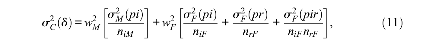
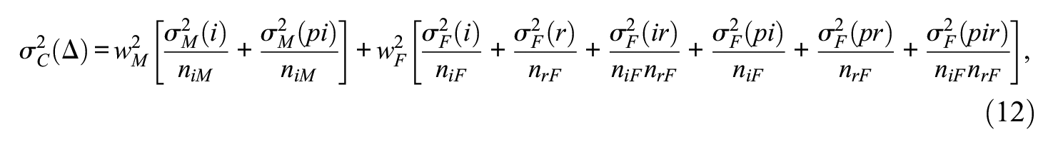
Similarly, absolute error variance for the composite is,

σ_{C}^{2} (Δ) = \sum_{υ} \sum_{υ'} w_{υ} w_{υ'} σ_{υ υ'} (Δ) .

(4)

Kane’s (1996) error–tolerance $(E / T)$ ratios are an easy and convenient way to characterize the magnitude of absolute and relative standard errors of measurement compared with some tolerance for error, which is often taken to be $σ_{C} (p)$ . Specifically, an error–tolerance ratio for $Δ$ is,

\frac{E_{Δ}}{T} = \frac{σ_{C} (Δ)}{σ_{C} (p)},

(5)

which provides an indicator of the extent to which the absolute standard error of measurement (SEM) is large relative to the standard deviation of universe scores, where universe scores are what we would like to know about examinees. Similarly, an error–tolerance ratio for $δ$ is,

\frac{E_{δ}}{T} = \frac{σ_{C} (δ)}{σ_{C} (p)} .

(6)

The error–tolerance ratios in Equations 5 and 6 have corresponding reliability-like coefficients, called an index of dependability $(Φ)$ and a generalizability coefficient $(E ρ^{2})$ , respectively. (Note that italicized boldface $E$ in $E ρ^{2}$ should not be confused with the error term E). These coefficients are,

Φ = \frac{σ_{C}^{2} (p)}{σ_{C}^{2} (p) + σ_{C}^{2} (Δ)},

(7)

and

E ρ^{2} = \frac{σ_{C}^{2} (p)}{σ_{C}^{2} (p) + σ_{C}^{2} (δ)} .

(8)

It is easy to show that $\sqrt{(1 - Φ) / Φ} = E_{Δ} / T$ and $\sqrt{(1 - E ρ^{2}) / E ρ^{2}} = E_{δ} / T$ , but $E / T$ ratios are much simpler to understand.¹ Coefficients are not metric dependent in a linear sense; neither are $E / T$ ratios.

Example I: Mixed-Format Tests

Mixed-format tests are usually defined as having both MC and FR items, with examinee responses to the FR items evaluated by raters. Estimating error variances for mixed-format tests is relatively complicated compared with single-format tests. Primarily, this complexity arises because the use of different item formats introduces multiple different sources of error. As discussed next, this complexity can be addressed in a principled way through an expanded use of MGT.

AP German Language Exam

This example uses data from the AP German Language exam administered in 2013. This exam is a mixed-format test that consists of MC and FR items. The exam has 65 MC items scored 0 or 1, and 4 FR items scored 0 through 5. For the German exam, a composite score is defined as a weighted sum of the MC and FR section scores with a set of pre-specified section weights.

The section weights are established a priori by the College Board to achieve an intended proportion of points for each section. We use the term “relative weights” to refer to the proportional contributions to the composite score, in keeping with the terminology used by Powers and Brennan (2009). For AP German Language, the pre-specified relative weights were 0.5 for both MC and FR sections. That is, the test developers’ intent was that each section contributes 50% to the composite score, which ranges from 0 to 130. In other words, the College Board wants 65 points associated with each of the two sections. Note that the AP data used in this article are for illustrative purposes, only.

G theory analyses are usually conducted using the mean score metric. Let ${\bar{X}}_{M}$ and ${\bar{X}}_{F}$ be the examinee mean scores for the MC and FR sections, respectively. The composite score can be defined as $C = w_{M} {\bar{X}}_{M} + w_{F} {\bar{X}}_{F}$ , where $w_{M}$ and $w_{F}$ are the “nominal” weights for the MC and FR sections, respectively, such that (a) the relative weights are .5 for both sections and (b) the maximum score for $C$ is 130. As the maximum values of ${\bar{X}}_{M}$ and ${\bar{X}}_{F}$ are 1 and 5, respectively, and $w_{M} {\bar{X}}_{M} = w_{F} {\bar{X}}_{F}$ to satisfy the requirement that both sections contribute an equal number of points to the maximum composite, it follows that $w_{M} = 65$ and $w_{F} = 65 / 5 = 13 .$ Brennan (2016a) provides additional details on how to determine weights.

Universe of Admissible Observations and Associated G Studies

Let $p$ , $i$ , and $r$ stand for persons, items, and raters, respectively. One way to characterize the UAO is to say it is the conjunction of two universes—one that involves MC items and one that involves FR items and raters. With the same population of persons responding to both types of items, we might denote this as ${p^{•} \times i} {p^{•} \times i \times r}$ , where the superscript bullet signifies that the same set of persons responds to both types of items, and it is assumed that, in principle, each rater could rate every item. The two sets of braces signify that there are two levels (MC and FR) of the fixed facet. We can denote this design somewhat more succinctly as $p^{•} \times [i ° \cup (i ° \times r °)]$ , where ∪ means the union of the two levels of the fixed facet (MC and FR), and the superscript open circle signifies that the measurement conditions (items and raters) are different for MC and FR. Given this notational system, the square brackets encompass the UAO with persons being the objects of measurement. (Note that $i$ is used here to designate either MC or FR items; the context determines the meaning).

G Study Designs

For the AP German Language exam, each FR item is scored by a single rater, which makes it impossible to disentangle the variability attributable to raters and items. This is an example of the so-called “problem of one” discussed by Brennan (2016b). Even though the rater and item facets are both conceptualized as being random and crossed in the UAO, the G study design, using single ratings of FR items for the operational data, fails to reflect the structure of the UAO.

Unfortunately, the usual way of addressing this complexity is to pretend that it does not exist (or does not matter) and simply conduct an MGT analysis using the $p^{•} \times i^{°}$ design, which hides the fact that for FR items, item effects and rater effects are completely confounded. The $p^{•} \times i^{°}$ design is considered here as a kind of typical, baseline analysis, the results for which are ambiguous. To examine these ambiguities, using a special study, two additional MGT analyses are considered here. One analysis uses the $p^{•} \times [i ° \cup (i ° \times r °)]$ design, and the other uses the $p^{•} \times [i ° \cup (r ° : i °)]$ design. These designs are discussed next. (Note that, for both designs, the MC and FR items are different.)

$p^{•} \times i^{°}$ Design

For the G study $p^{•} \times i^{°}$ design, there is a different set of items in each level of the fixed facet (MC and FR), and for FR items, there is only a single rater (or rating) for each item. When this design is used in the mixed-format context, raters are effectively a hidden facet. That is, basically, it is assumed that there is a single rater (or rating) for each person-item combination, but the design is agnostic with respect to the actual number of raters involved and how they were assigned to persons and items. The left part of Table 1 shows a Venn diagram representation of the $p^{•} \times i^{°}$ design, with a dashed circle indicating the fixed facet, with the two levels being MC and FR.

Table 1.

Example I: G Study $p^{•} \times i °$ Design and the D Study $p^{•} \times I °$ Design.

Venn Diagram	G Study	D Study
	${\hat{Σ}}_{p} = [\begin{matrix} 0.03156 & 0.17405 \\ 0.17405 & 1.08177 \end{matrix}]$ ${\hat{Σ}}_{i} = [\begin{matrix} . 02630 \\ . 04532 \end{matrix}]$ ${\hat{Σ}}_{pi} = [\begin{matrix} . 17469 \\ . 62499 \end{matrix}]$	${\hat{Σ}}_{p} = [\begin{matrix} 0.03156 & 0.17405 \\ 0.17405 & 1.08177 \end{matrix}]$ ${\hat{Σ}}_{I} = [\begin{matrix} . 00040 \\ . 01133 \end{matrix}]$ ${\hat{Σ}}_{pI} = [\begin{matrix} . 00269 \\ . 15625 \end{matrix}]$ ${\hat{Σ}}_{δ} = [\begin{matrix} . 00269 \\ . 15625 \end{matrix}]$ ${\hat{Σ}}_{Δ} = [\begin{matrix} . 00310 \\ . 16758 \end{matrix}]$

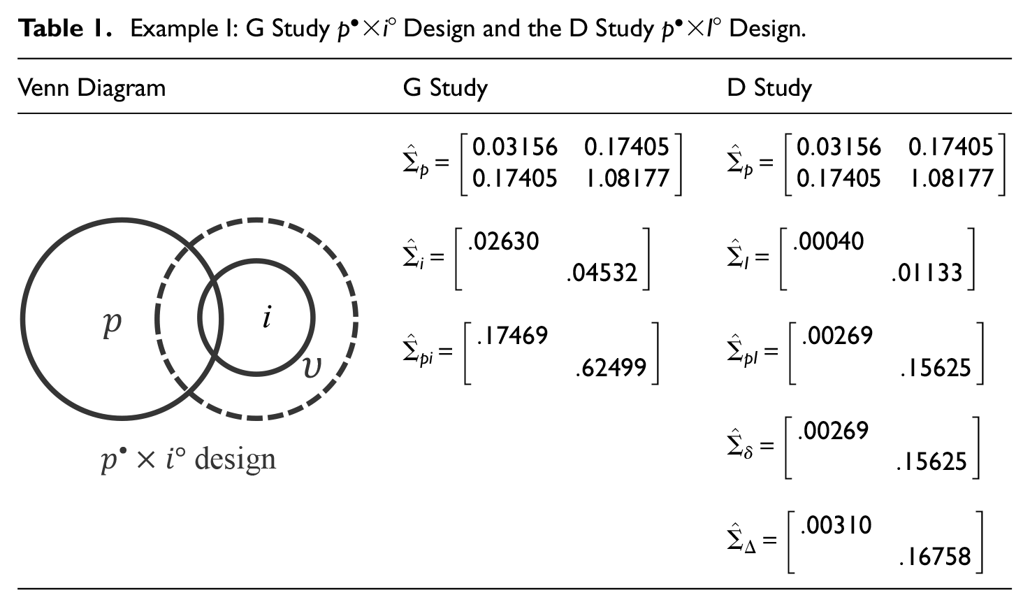
For the German Exam considered here, we can denote this G study design more explicitly as $p^{•} \times [i ° \cup (i °, r °)]$ , where $(i °, r °)$ designates that FR items and raters are completely confounded for the FR section. Note, in particular, however, that in the UAO almost certainly items and raters are distinguishable, and they are both random. In this sense, there are both ambiguities and conceptual disconnects between the UAO and the G study design.

For example, if the same rater actually rated all FR items for all examinees, then the rater facet would be both hidden and fixed, as far as the G study is concerned. If a single different rater rated all FR items for all examinees, then the rater facet would be hidden and random. In any case, for a G study $p^{•} \times i^{°}$ design (with raters hidden), it is impossible to disentangle rater effects from effects attributable to persons and items, even though rater effects are distinguishable in the UAO. This type of mismatch leads to interpretational complexities and ultimately bias (almost certainly) in certain D study statistics (see Brennan, 2016b), including error variances, error–tolerance ratios, and reliability-like coefficients. In this sense, if the only data available conform to a $p^{•} \times i^{°}$ G study design, then statistical results are likely to be suspect relative to the actual UAO and the intended UG.

$p^{•} \times [i ° \cup (i ° \times r °)]$ Design

Table 2 considers the $p^{•} \times [i ° \cup (i ° \times r °)]$ design for the German Exam. Specifically, the two Venn diagrams on the left side of the table depict the design structure for the two fixed levels: $p \times i$ for the MC section and $p \times i \times r$ for the FR section.

Table 2.

Example I: G Study $p^{•} \times [i ° \cup (i ° \times r °)]$ Design and Companion D Study Design.

Venn Diagram	G Study	D Study
MC Section $p \times i$ design FR Section $p \times i \times r$ design	${\hat{Σ}}_{p} = [\begin{matrix} 0.03156 & 0.17334 \\ 0.17334 & 1.14914 \end{matrix}]$ ${\hat{Σ}}_{i} = [\begin{matrix} . 02630 \\ . 04040 \end{matrix}]$ ${\hat{Σ}}_{r} = [\begin{matrix} - - - \\ - . 01313 \end{matrix}]$ ${\hat{Σ}}_{pi} = [\begin{matrix} . 17479 \\ . 26091 \end{matrix}]$ ${\hat{Σ}}_{pr} = [\begin{matrix} - - - \\ - . 00072 \end{matrix}]$ ${\hat{Σ}}_{ir} = [\begin{matrix} - - - \\ . 04342 \end{matrix}]$ ${\hat{Σ}}_{pir} = [\begin{matrix} - - - \\ . 30332 \end{matrix}]$	${\hat{Σ}}_{p} = [\begin{matrix} 0.03156 & 0.17334 \\ 0.17334 & 1.14914 \end{matrix}]$ ${\hat{Σ}}_{I} = [\begin{matrix} . 00040 \\ . 01010 \end{matrix}]$ ${\hat{Σ}}_{R} = [\begin{matrix} - - - \\ 0 \end{matrix}]$ ${\hat{Σ}}_{pI} = [\begin{matrix} . 00269 \\ . 06523 \end{matrix}]$ ${\hat{Σ}}_{pR} = [\begin{matrix} - - - \\ 0 \end{matrix}]$ ${\hat{Σ}}_{IR} = [\begin{matrix} - - - \\ . 01085 \end{matrix}]$ ${\hat{Σ}}_{pIR} = [\begin{matrix} - - - \\ . 07583 \end{matrix}]$ ${\hat{Σ}}_{δ} = [\begin{matrix} . 00269 \\ . 14105 \end{matrix}]$ ${\hat{Σ}}_{Δ} = [\begin{matrix} . 00310 \\ . 16200 \end{matrix}]$

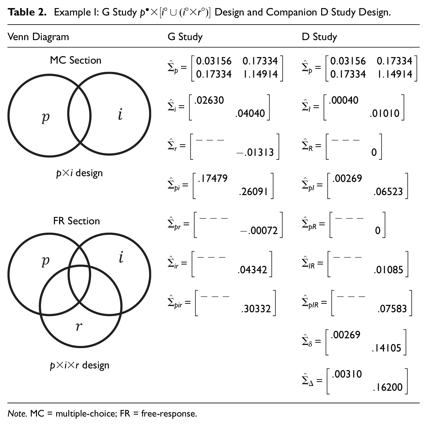
Note. MC = multiple-choice; FR = free-response.

This second MGT design is rarely seen in the literature, although it is quite similar to that discussed by Moses and Kim (2015). Specifically, they suggested an MGT design for mixed-format tests, which they denoted $p^{•} \times (i ° or j °) \times h^{°}$ . In their notation, the $i$ and $j$ items ( $i$ for FR, $j$ for MC) are nested within item format (a fixed variable), whereas the rating $(h)$ facet is defined for FR items, only. In their study, ratings, not raters, were designated as a facet. By contrast, in the present study, data from a special study (discussed later) permitted a further investigation of rater effects. Otherwise, however, the $p^{•} \times [i ° \cup (i ° \times r °)]$ design considered here is virtually identical to that used by Moses and Kim (2015).

$p^{•} \times [i ° \cup (r ° : i °)]$ Design

This third design is different from the second design in that raters are nested within items as opposed to being crossed. It follows that some variance components in the crossed UAO are confounded in estimated variance components for this nested design. As illustrated later, this confounding typically leads to smaller error variances than for the crossed design (see, also, Brennan, 2001a). Venn diagrams pertaining to the $p^{•} \times [i ° \cup (r ° : i °)]$ design are provided on the left side of Table 3. Importantly, note that each FR item is evaluated by a different set of raters, as reflected by the Venn diagram in the lower-left of Table 3.

Table 3.

Example I: G Study $p^{•} \times [i ° \cup (r ° : i °)]$ Design and Companion D Study Design.

Venn Diagram	G Study	D Study
MC Section $p \times i$ designFR Section $p \times (r : i)$ design	${\hat{Σ}}_{p} = [\begin{matrix} 0.03156 & 0.17334 \\ 0.17334 & 1.07066 \end{matrix}]$ ${\hat{Σ}}_{i} = [\begin{matrix} . 02630 \\ . 07576 \end{matrix}]$ ${\hat{Σ}}_{r : i} = [\begin{matrix} - - - \\ . 03030 \end{matrix}]$ ${\hat{Σ}}_{pi} = [\begin{matrix} . 17479 \\ . 33939 \end{matrix}]$ ${\hat{Σ}}_{pr : i} = [\begin{matrix} - - - \\ . 30260 \end{matrix}]$	${\hat{Σ}}_{p} = [\begin{matrix} 0.03156 & 0.17334 \\ 0.17334 & 1.07066 \end{matrix}]$ ${\hat{Σ}}_{I} = [\begin{matrix} . 00041 \\ . 01894 \end{matrix}]$ ${\hat{Σ}}_{R : I} = [\begin{matrix} - - - \\ . 03030 \end{matrix}]$ ${\hat{Σ}}_{pI} = [\begin{matrix} . 00269 \\ . 08485 \end{matrix}]$ ${\hat{Σ}}_{pR : I} = [\begin{matrix} - - - \\ . 07565 \end{matrix}]$ ${\hat{Σ}}_{δ} = [\begin{matrix} . 00269 \\ . 16050 \end{matrix}]$ ${\hat{Σ}}_{Δ} = [\begin{matrix} . 00310 \\ . 20973 \end{matrix}]$

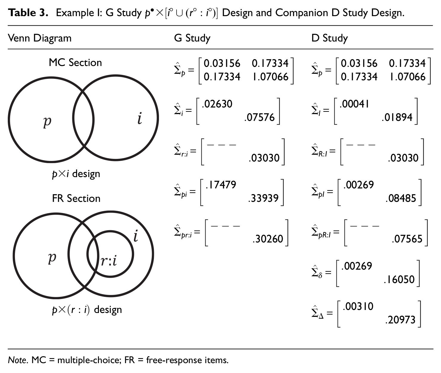
Note. MC = multiple-choice; FR = free-response items.

Data

For this study, three sets of data were obtained: one from the operational administration and the other two from a special study conducted by the College Board. As noted previously, operationally, an examinee’s response to each of the four FR items is evaluated by a single rater. Consequently, the unconfounded effect of rater variability cannot be studied using the operational data, alone. For this reason, a special study was conducted to obtain additional ratings for each FR item for a subset of the examinees. Doing so facilitated examining rater effects—in particular, their impact on estimated error variances and related statistics.

Figure 1 depicts the structure of the operational data (first column) and the two subsets of data for the special study (two lower-right cells). The operational MC data are labeled ①, the operational FR ratings are labeled ②, and the special study FR ratings are labeled ③ and ④.

Figure 1.

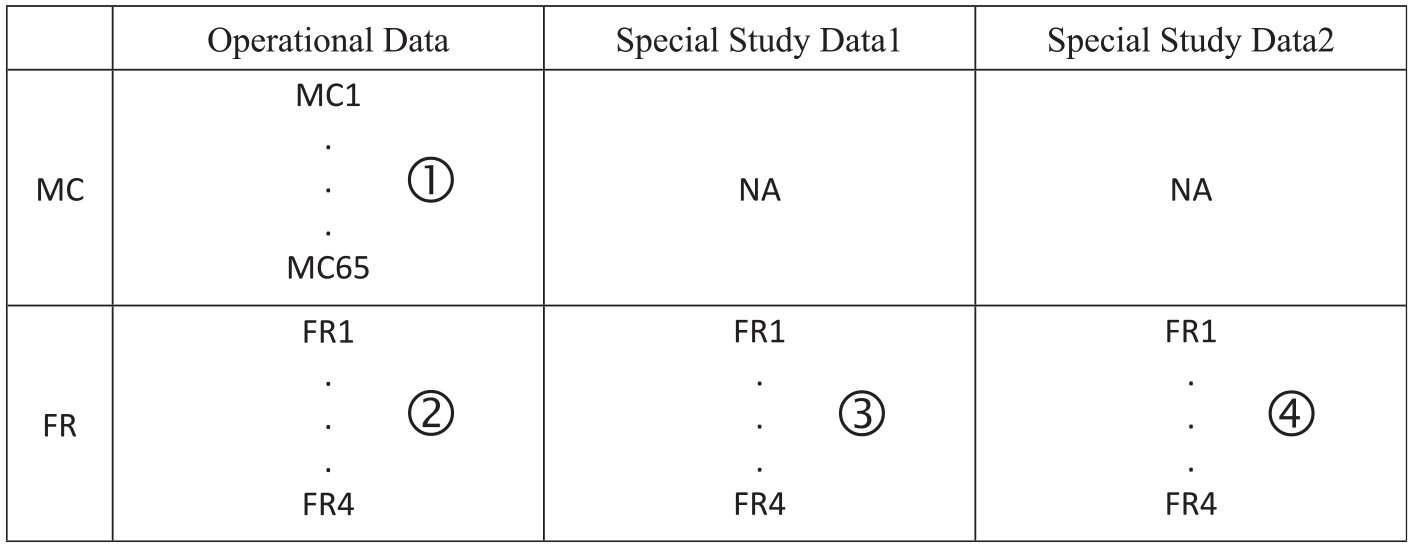
Data Structure for the Three Datasets in Example I.

For the special study, FR answer books for 109 examinees were selected from the operational administration. To make the rating task manageable, these 109 examinees were split into approximately equal subsets (denoted P1–P55 and P56–P109). For each person, each FR item was scored by two additional raters in the manner indicated in Figure 2. (Note that the identifiers R1 to R8 in Figure 2 designate different raters, not simply different ratings.) In short, the word “Folder” in Figure 2 is a designator for a set of data associated with a set of persons, a pair of raters, and a single FR item.

Figure 2.

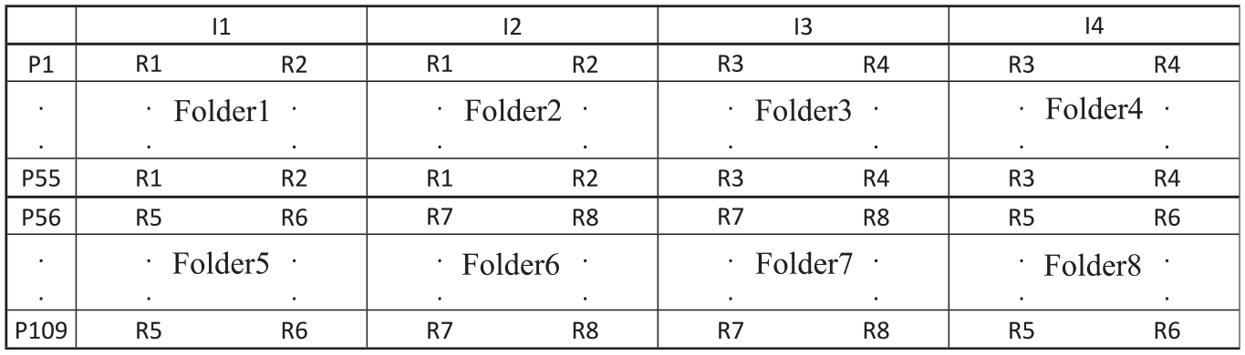
Venn Diagrams for G Study $p^{•} \times i °$ and $p^{•} \times [2 (i ° : h °) \cup 2 (i)]$ Designs.

Clearly, the special study does not conform to a fully crossed or fully nested design, but carefully selected subsets of the data do conform to a crossed or nested design. Specifically, four pairs of folders provide data for persons crossed with raters crossed with items—specifically, Folders 1 and 2, 3 and 4, 5 and 8, and 6 and 7. By contrast, four different pairs of folders provide data for persons crossed with raters nested within items—specifically, Folders 1 and 3, 2 and 4, 5 and 6, and 7 and 8. Consequently, as discussed below, it was possible to examine three G theory designs: one that conforms with the operational administration and two that provide different perspectives on rater effects.

$p^{•} \times i^{°}$ Design

As there were three FR scores available for each FR item based on the operational administration and special study (i.e., ②,③, and ④ in Figure 1), three separate $p^{•} \times i^{°}$ G study analyses were conducted to obtain three sets of estimated G study variance and covariance components (i.e., ①+②, ①+③, and ①+④ in Figure 1). The averaged values over the three analyses were treated as final estimates, which were then used as input to obtain D study results using mGENOVA (Brennan, 2001b). (Note that, for this design and the subsequent two designs, there is only one set of variance components for MC items, designated ① in Figure 1.)

$p^{•} \times [i ° \cup (i ° \times r °)]$ Design

For the second G study design, $p^{•} \times [i ° \cup (i ° \times r °)]$ , univariate analyses were conducted for the MC and FR sections separately using GENOVA (Crick & Brennan, 1983). For the full multivariate design, hand calculation was used to obtain the only required estimated covariance, specifically,

{\hat{σ}}_{MF} (p) = S_{MF} (p) = \frac{n_{p}}{n_{p} - 1} (\frac{\sum_{p} {\bar{X}}_{pM} {\bar{X}}_{pF}}{n_{p}} - {\bar{X}}_{M} {\bar{X}}_{F}),

(9)

where $M$ and $F$ stand for MC and FR, respectively, and replace $υ$ and $υ'$ in Equation 1. Also, using Equations 2 to 4, universe score variance, relative error variance, and absolute error variance for the composite scores were estimated as follows:

σ_{C}^{2} (p) = w_{M}^{2} σ_{M}^{2} (p) + w_{F}^{2} σ_{F}^{2} (p) + 2 w_{M} w_{F} σ_{MF} (p),

(10)

σ_{C}^{2} (δ) = w_{M}^{2} [\frac{σ_{M}^{2} (pi)}{n_{iM}}] + w_{F}^{2} [\frac{σ_{F}^{2} (pi)}{n_{iF}} + \frac{σ_{F}^{2} (pr)}{n_{rF}} + \frac{σ_{F}^{2} (pir)}{n_{iF} n_{rF}}],

(11)

and

σ_{C}^{2} (Δ) = w_{M}^{2} [\frac{σ_{M}^{2} (i)}{n_{iM}} + \frac{σ_{M}^{2} (pi)}{n_{iM}}] + w_{F}^{2} [\frac{σ_{F}^{2} (i)}{n_{iF}} + \frac{σ_{F}^{2} (r)}{n_{rF}} + \frac{σ_{F}^{2} (ir)}{n_{iF} n_{rF}} + \frac{σ_{F}^{2} (pi)}{n_{iF}} + \frac{σ_{F}^{2} (pr)}{n_{rF}} + \frac{σ_{F}^{2} (pir)}{n_{iF} n_{rF}}],

(12)

where $w_{M}$ = 65 and $w_{F}$ = 13. Error–tolerance ratios and coefficients were computed using Equations 5 to 8. All facets, including persons, items, and raters were treated as random.

Recall that, for the special study, four pairs of folders provide data for persons crossed with raters crossed with items—specifically, Folders 1 and 2, 3 and 4, 5 and 8, and 6 and 7. For each of these pairs of folders, the design is $p \times i \times r$ with two items, two raters, and either 55 or 54 persons. Each of these four pairs of folders is considered to be a pseudo-replication. Strictly speaking, they are not “pure” replications as some replications involved the same persons.

D study statistics were computed using the average of the estimated variance components for these four replications or subsets, with the expectation that these averages would serve as more accurate estimates than estimates from a single subset. (The MC estimated variance components are the same as those in Table 1). The operational responses to the FR items (② in Figure 1) could not be used in this analysis because rater information was not available. Negative variance component estimates were retained for the pseudo-replications, but average variance components (over replications) that were negative were set to zero.

$p^{•} \times [i ° \cup (r ° : i °)]$ Design

For this design, the same basic approach was used as for the crossed design. The only difference is that the pairs of folders for the FR part of the $p^{•} \times [i ° \cup (r ° : i °)]$ design were Folders 1 and 3, 2 and 4, 5 and 6, and 7 and 8—that is, pairs of folders for which pairs of FR items were scored by different pairs of raters. For instance, combining Folders 1 and 3 provided data for a $p \times (r : i)$ design in which each of two items was scored by a different pair of raters. Again, final results were obtained by averaging estimated variance components over pairs of folders.

Estimated G and D Study Variance and Covariance Components

The estimated G study and D study variance–covariance components based on the $p^{•} \times i^{°}$ design are provided in the middle and right parts of Table 1, respectively. Results for the G and D studies include 2 × 2 matrices for each facet with rows and columns ordered as MC and FR. The diagonal elements in each matrix are estimated variance components and the off-diagonal elements are estimated covariance components. The D study estimated variance–covariance components were obtained by dividing their corresponding G study components by the sample sizes ( $n_{iM}^{'}$ = 65, $n_{iF}^{'}$ = 4, or their product, as appropriate). The last two D study matrices provide estimates of relative and absolute error variances.

The middle and right parts of Table 2 show the estimated G study and D study variance–covariance matrices for the $p^{•} \times [i ° \cup (i ° \times r °)]$ design. Note that for MC items, matrices involving $r$ have “―――” in cell (1,1) indicating that variance components for raters are not relevant for the MC section. D study estimated variance components were obtained in a manner similar to that for the $p^{•} \times i^{°}$ design. The covariance component in ${\hat{Σ}}_{p}$ was estimated using Equation 9. Note that for the sake of simplicity, only results based on a single rater are presented. A similar approach was taken to compute the G study and D study variance–covariance components in Table 3 for the $p^{•} \times [i ° \cup (r ° : i °)]$ design.

The focus of Example I is on rater effects. To simplify design notation here, let the $p^{•} \times i °$ design be denoted D0, let the $p^{•} \times [i ° \cup (i ° \times r °)]$ crossed design be denoted DC, and let the $p^{•} \times [i ° \cup (r ° : i °)]$ partially nested design be denoted DN. For D0, raters are completely confounded with items and persons in an unknown manner such that we cannot isolate rater effects. That, in essence, is a central motivation for considering this example. For DC, ${\hat{σ}}_{F}^{2} (r)$ is essentially 0 (technically a negative number rounded to 0) suggesting that, on average (i.e., over items), there is very little variability among rater scores. However, ${\hat{σ}}_{F}^{2} (ir) = . 04342$ suggests that there is some (small) variability among raters with respect to their ratings of individual items. For DN, ${\hat{σ}}_{F}^{2} (r : i) = . 03030$ , which also suggests that there is some variability in rater scores for any (randomly selected) item. On balance, the estimated rater variance components for the more complicated designs (DC and DN) do not suggest that rater variability is a substantial problem, but without examining the more complicated designs, we could not know this.

Composite Summary Statistics

It is important to note that the estimated variance and covariance components in Tables 1 to 3 are for single persons, single items, and single raters. That is one reason why the numbers are very small in absolute magnitude. Obviously, our ultimate interest is in the 0 to 130 composite-score metric discussed previously. The first three rows in Table 4 provide relevant statistics for this metric. Specifically, these rows provide estimated standard deviations of person universe scores, absolute errors, and relative errors. The next two rows provide estimated error–tolerance ratios, and the last two rows provide estimated coefficients. Both coefficients necessarily range from 0 to 1. Both error–tolerance ratios usually have the same range, although they have substantially different interpretations, as discussed previously.

Table 4.

Example I: D Study Composite-Score Statistics.

	$p^{•} \times I^{°}$	$p^{•} \times [i^{°} \cup (i^{°} \times r^{°})]$		$p^{•} \times [i^{°} \cup (r^{°} : i^{°})]$
Statistic	$n_{r}^{'}$ = 1	$n_{r}^{'}$ = 1	$n_{r}^{'}$ = 2	$n_{r}^{'}$ = 1	$n_{r}^{'}$ = 2
${\hat{σ}}_{C} (p)$	24.704	24.910	24.910	24.642	24.642
${\hat{σ}}_{C} (Δ)$	6.436	6.362	5.758	6.681	6.134
${\hat{σ}}_{C} (δ)$	6.146	5.933	5.366	6.204	5.666
Est $(\frac{E_{Δ}}{T})$	.261	.255	.231	.271	.249
Est $(\frac{E_{δ}}{T})$	.249	.238	.215	.272	.230
Est $(Φ)$	.937	.939	.949	.931	.942
Est $(E ρ^{2})$	.942	.946	.956	.940	.950

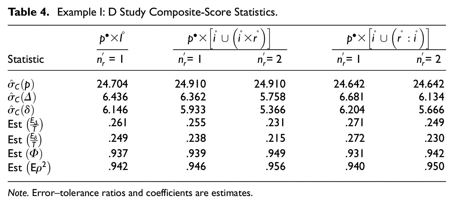
Note. Error–tolerance ratios and coefficients are estimates.

Results are reported for all three designs. The second column provides results for the D0 operational design. DC and DN results are provided for D study sample sizes of both $n'_{r} = 1$ and $n'_{r} = 2$ raters. Note that for D0, there is only one rating of each examinee’s response for each FR item, but there are many raters involved, with an unknown assignment procedure of raters to persons and FR items. For DC and DN, there is more specificity. For example, DC with $n'_{r} = 2$ means that there are two randomly selected raters who evaluate the responses of all persons to randomly selected FR items. By contrast, DN with $n'_{r} = 2$ means that there are two different raters for each item.

There are at least two principal results in Table 4. First, as the number of raters increases, both ${\hat{σ}}_{C} (Δ)$ and ${\hat{σ}}_{C} (δ)$ decrease, which leads to corresponding decreases in estimated error–tolerance ratios and increases in coefficients. Second, the magnitude of the decreases/increases is not notably large; indeed, the DC and DN results with $n'_{r} = 1$ are not much different from the operational results (D0), which lends support to the current rating procedures.

The data sets for the three designs in Table 4 overlap, but, as discussed previously, the data were manipulated differently to conform with the different designs. Consequently, the results for one design are not entirely predictable from the results for any other design.² Furthermore, estimates of variance components (and functions of them) are themselves subject to sampling variability (see Brennan, 2001a), which can distort results somewhat. These facts are associated with some anomalies in the Table 4 results. For example, for any particular $n'_{r}$ , we typically expect that ${\hat{σ}}_{C} (Δ)$ for DN will be less than ${\hat{σ}}_{C} (Δ)$ for DC, which is not always true in Table 4. For the present example, however, such inconsistencies are rather minor, which lends credence to the scoring procedures currently used. For example, estimated $E_{Δ} / T$ with $n'_{r} = 1$ is in the range of about .26 to .27 for all three designs; with $n'_{r} = 2$ , the range is .23 to .25 for the DC and DN designs. Such differences, and the corresponding differences in coefficients, seem relatively minor for practical purposes. Still, as discussed below, an argument could be made that the DN design with $n'_{r} = 2$ might be worth considering for operational use.

For the operational D0 design and the more complicated DN design, the MC items are the same, and they do not involve any ratings. Therefore, for present purposes, we can focus exclusively on the four-item FR section for these two designs. Under the D0 design, for each person, there is a single rating for each item. The total number of raters involved is typically knowable, but the actual process of assigning raters to person and items is likely to be vague.

Strictly speaking, for the DN design with $n_{r}' = 2$ , there is a different pair of raters for each item (a total of eight raters). Furthermore, the same four pairs of raters are used for all persons, which is not realistic when the number of persons is large. An obvious alternative is to randomly split persons into some number of smaller, equally sized groups. Then, for each group, different randomly selected pairs of raters can be used to rate each item.³ Strictly speaking, the precise structure of this modified design is more complicated than $p^{•} \times [I ° \cup (R ° : I °)]$ , but the basic structural issues are intact, and the estimates in the last column of Table 4 are likely reasonable. This approach is expected to lead to improved measurement precision (over that provided by the D0 design), but the amount of improvement may or may not justify the time, effort, and cost involved.

Example II: Tests With Testlets

Items involving a common stimulus are usually bundled together. For such items, logic and research suggest that dependencies can exist. Consequently, it has been suggested that testlet effects be taken into consideration in measurement analyses to avoid possible underestimation of error variance and overestimation of reliability (Lee, 2000a, 2000b; Lee & Frisbie, 1999; Sireci et al., 1991).

Exam and Dataset

The second example uses the same exam as the first example, but with a different dataset. Unlike the previous example that examined rater effects, investigating testlet effects does not necessarily require a special study to collect data from multiple raters. Thus, data from a single administration to a large group were used in this example with a total sample size of 4,111.

The AP German Language exam was designed to measure four distinct skills: reading (R), listening (L), writing (W), and speaking (S). The R and L sections are composed of testlet-based items, only, while the W and S sections each consists of a separate stand-alone set of items. There are four testlets associated with R with 5, 7, 11, and 7 MC items in each testlet. Five testlets are used for L with 10, 7, 5, 5, and 8 MC items within each testlet. For each testlet, a common stimulus provides the basis for answering the items that belong to the testlet. For both W and S, there are two independent FR items scored 0 to 5. Note that there is only one rating per item, which means that FR items and ratings are completely confounded in the data.

Universe of Admissible Observations

The UAO is the conjunction of universes for R, L, W, and S. Letting $p$ , $i$ , and $h$ stand for persons, items, and testlets, respectively, we denote the structure of the UAO as $p^{•} \times [2 (i ° : h °) \cup 2 (i °)]$ where the first 2 refers to R and L, the second 2 refers to W and S. The superscript open circles indicate that the conditions of the facets differ for each of the fixed “levels” or sections (i.e., R, L, W, and S). Here, we are neglecting the fact that FR items in W and S are evaluated by raters.⁴ (Note that $i$ is used here to designate either MC items within testlets or stand-alone MC items; the context determines the meaning.)

Strictly speaking, the UAO is within square brackets, with the population of persons crossed with the UAO. The superscript closed circle associated with $p$ signifies that all persons in the population respond to all items in all four sections.

G Study $p^{•} \times i^{°}$ Design

Clearly, the G study design that mirrors the UAO is $p^{•} \times [2 (i ° : h °) \cup 2 (i °)]$ , which is admittedly complex. To simplify matters, analyses oftentimes ignore the effect of testlets, with items treated as an undifferentiated set for each level of the fixed facet. Accordingly, results for a traditional MGT $p^{•} \times i^{°}$ design are also considered in this article and compared with results for the $p^{•} \times [2 (i ° : h °) \cup 2 (i °)]$ design. (Venn Diagrams for these two designs are provided in Figure 3). A similar comparison was made by Lee and Frisbie (1999), but they compared results for univariate designs, only—specifically, the $p \times i$ and $p \times (i : h)$ designs. For the AP German Language dataset considered here, Table 5 provides $p \times i$ estimated variance and covariance components for the four sections (R, L, W, and S).

Table 5.

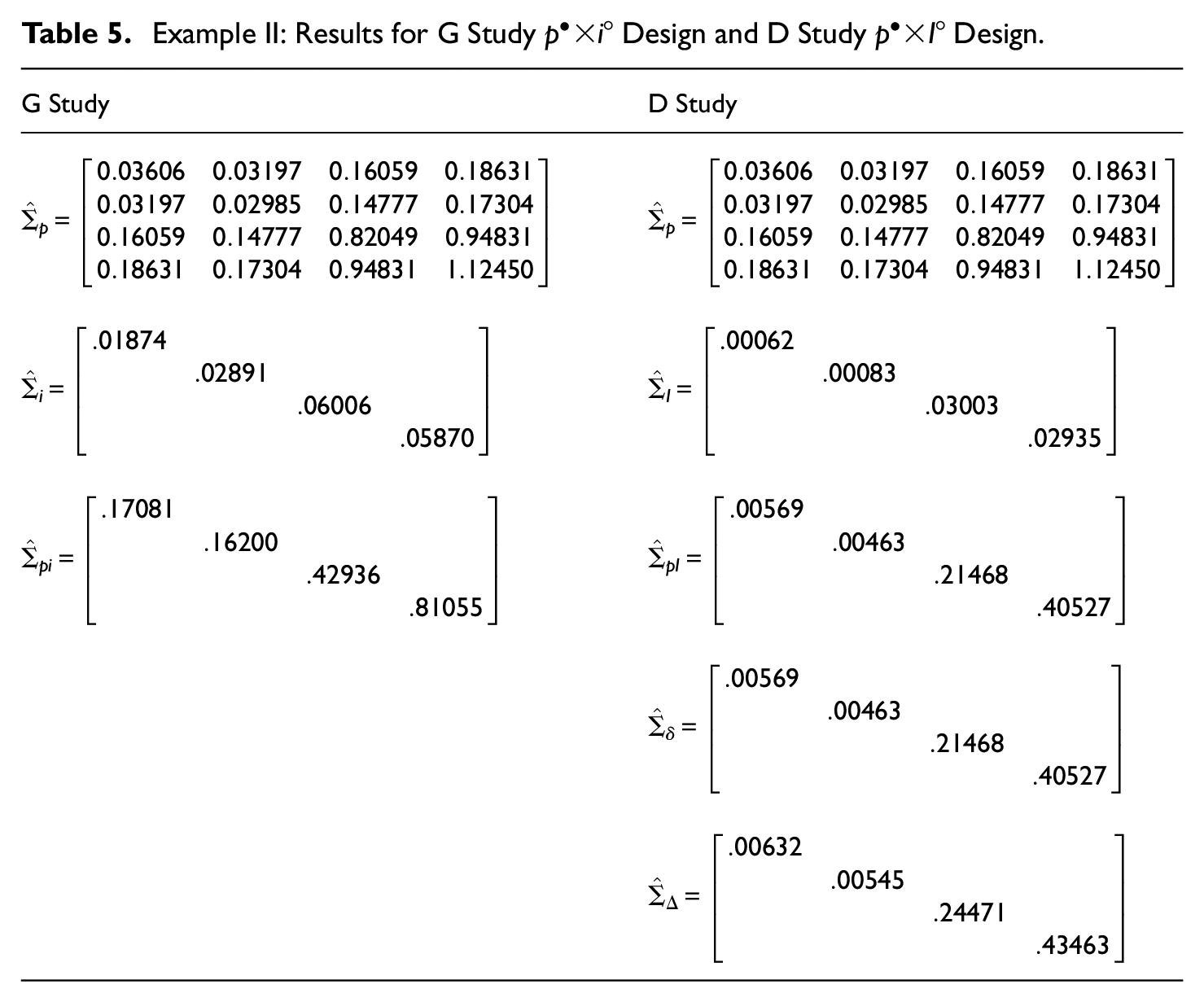
Example II: Results for G Study $p^{•} \times i °$ Design and D Study $p^{•} \times I °$ Design.

G Study	D Study
${\hat{Σ}}_{p} = [\begin{matrix} 0.03606 & 0.03197 & 0.16059 & 0.18631 \\ 0.03197 & 0.02985 & 0.14777 & 0.17304 \\ 0.16059 & 0.14777 & 0.82049 & 0.94831 \\ 0.18631 & 0.17304 & 0.94831 & 1.12450 \end{matrix}]$ ${\hat{Σ}}_{i} = [\begin{matrix} . 01874 \\ . 02891 \\ . 06006 \\ . 05870 \end{matrix}]$ ${\hat{Σ}}_{pi} = [\begin{matrix} . 17081 \\ . 16200 \\ . 42936 \\ . 81055 \end{matrix}]$	${\hat{Σ}}_{p} = [\begin{matrix} 0.03606 & 0.03197 & 0.16059 & 0.18631 \\ 0.03197 & 0.02985 & 0.14777 & 0.17304 \\ 0.16059 & 0.14777 & 0.82049 & 0.94831 \\ 0.18631 & 0.17304 & 0.94831 & 1.12450 \end{matrix}]$ ${\hat{Σ}}_{I} = [\begin{matrix} . 00062 \\ . 00083 \\ . 03003 \\ . 02935 \end{matrix}]$ ${\hat{Σ}}_{pI} = [\begin{matrix} . 00569 \\ . 00463 \\ . 21468 \\ . 40527 \end{matrix}]$ ${\hat{Σ}}_{δ} = [\begin{matrix} . 00569 \\ . 00463 \\ . 21468 \\ . 40527 \end{matrix}]$ ${\hat{Σ}}_{Δ} = [\begin{matrix} . 00632 \\ . 00545 \\ . 24471 \\ . 43463 \end{matrix}]$

G Study

D Study

{\hat{Σ}}_{p} = [\begin{matrix} 0.03606 & 0.03197 & 0.16059 & 0.18631 \\ 0.03197 & 0.02985 & 0.14777 & 0.17304 \\ 0.16059 & 0.14777 & 0.82049 & 0.94831 \\ 0.18631 & 0.17304 & 0.94831 & 1.12450 \end{matrix}]

{\hat{Σ}}_{i} = [\begin{matrix} . 01874 \\ . 02891 \\ . 06006 \\ . 05870 \end{matrix}]

{\hat{Σ}}_{pi} = [\begin{matrix} . 17081 \\ . 16200 \\ . 42936 \\ . 81055 \end{matrix}]

{\hat{Σ}}_{p} = [\begin{matrix} 0.03606 & 0.03197 & 0.16059 & 0.18631 \\ 0.03197 & 0.02985 & 0.14777 & 0.17304 \\ 0.16059 & 0.14777 & 0.82049 & 0.94831 \\ 0.18631 & 0.17304 & 0.94831 & 1.12450 \end{matrix}]

{\hat{Σ}}_{I} = [\begin{matrix} . 00062 \\ . 00083 \\ . 03003 \\ . 02935 \end{matrix}]

{\hat{Σ}}_{pI} = [\begin{matrix} . 00569 \\ . 00463 \\ . 21468 \\ . 40527 \end{matrix}]

{\hat{Σ}}_{δ} = [\begin{matrix} . 00569 \\ . 00463 \\ . 21468 \\ . 40527 \end{matrix}]

{\hat{Σ}}_{Δ} = [\begin{matrix} . 00632 \\ . 00545 \\ . 24471 \\ . 43463 \end{matrix}]

Figure 3.

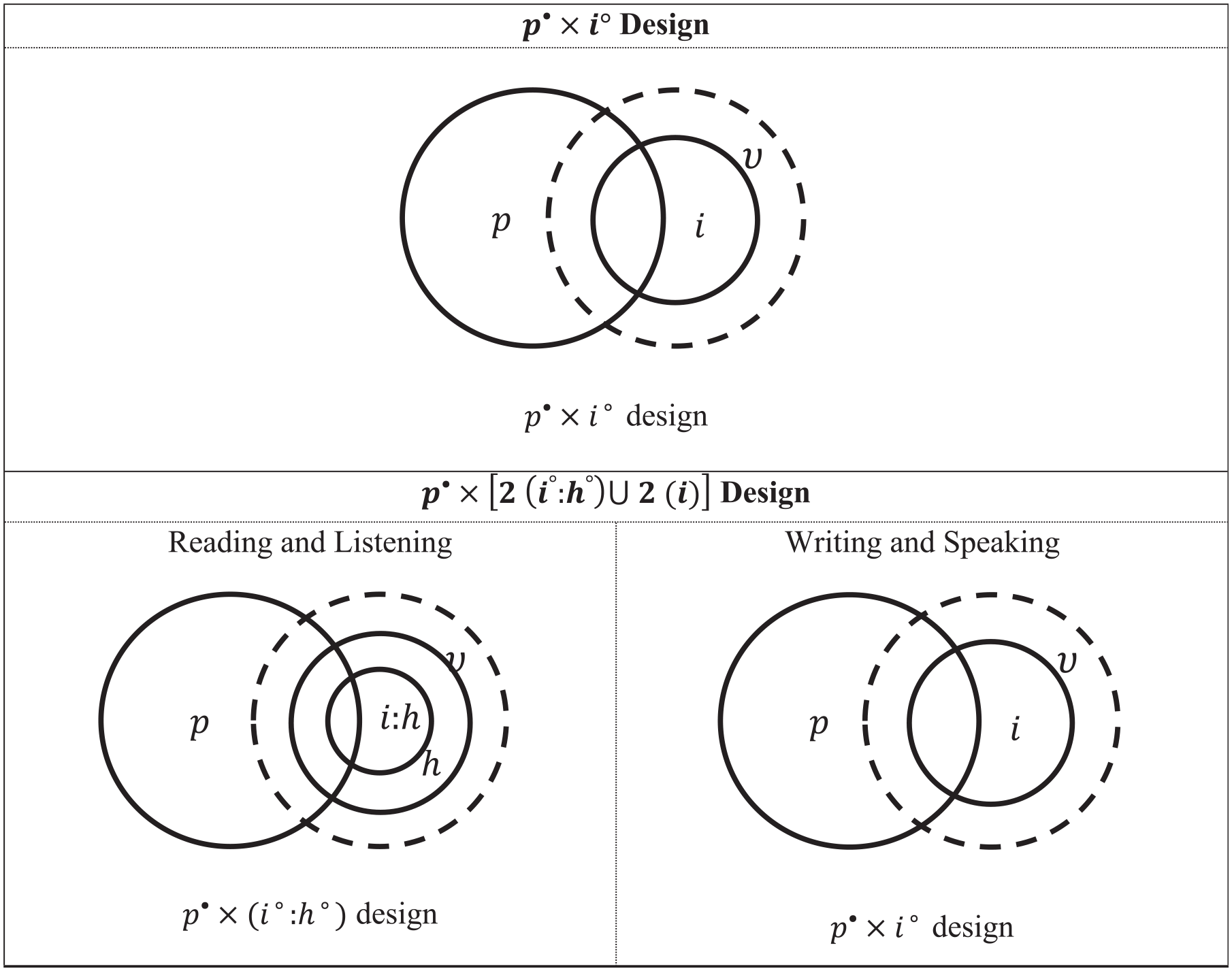
Venn Diagrams for G Study $p^{•} \times i^{°}$ and $p^{•} \times [2 (i^{°} : h^{°}) \cup 2 (i^{°})]$ Designs.

G Study $p^{•} \times [2 (i ° : h °) \cup 2 (i °)]$ Design

The G study $p^{•} \times [2 (i ° : h °) \cup 2 (i °)]$ design has not been treated in the existing literature. It is complex, but it can be described rather simply. Specifically, this design is the conjunction of two traditional MGT designs: a $p^{•} \times (i ° : h °)$ design for the R and L sections, and a $p^{•} \times i °$ design for the W and S sections.

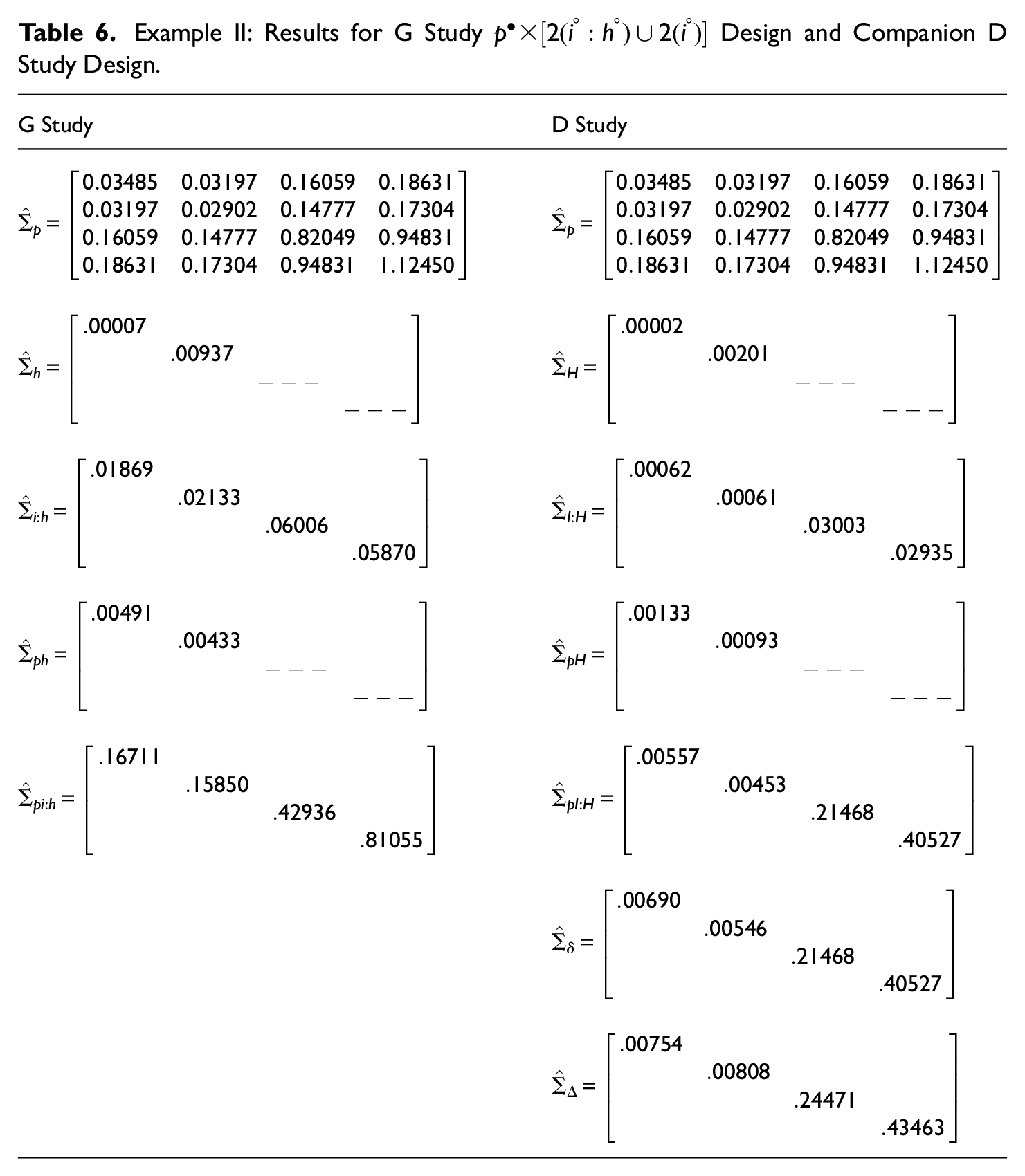
This two sub-designs perspective implies that the following steps can be used to estimate variance components and covariance components for the “full” $p^{•} \times [2 (i : h) U 2 (i)]$ design: (i) use mGENOVA (Brennan, 2001b) to estimate variance and covariance components for R and L for the $p^{•} \times (i ° : h °)$ sub-design; (ii) use mGENOVA to estimate variance and covariance components for W and S for the $p^{•} \times i °$ sub-design; and (iii) use Equation 1 to obtain estimates of the four across-design covariance components, that is, ( ${\hat{σ}}_{RW} (p)$ , ${\hat{σ}}_{RS} (p)$ , ${\hat{σ}}_{LW} (p)$ , ${\hat{σ}}_{LS} (p)$ ). These results are provided in Table 6.

Table 6.

Example II: Results for G Study $p^{•} \times [2 (i^{°} : h^{°}) \cup 2 (i^{°})]$ Design and Companion D Study Design.

G Study	D Study
${\hat{Σ}}_{p} = [\begin{matrix} 0.03485 & 0.03197 & 0.16059 & 0.18631 \\ 0.03197 & 0.02902 & 0.14777 & 0.17304 \\ 0.16059 & 0.14777 & 0.82049 & 0.94831 \\ 0.18631 & 0.17304 & 0.94831 & 1.12450 \end{matrix}]$ ${\hat{Σ}}_{h} = [\begin{matrix} . 00007 \\ . 00937 \\ - - - \\ - - - \end{matrix}]$ ${\hat{Σ}}_{i : h} = [\begin{matrix} . 01869 \\ . 02133 \\ . 06006 \\ . 05870 \end{matrix}]$ ${\hat{Σ}}_{ph} = [\begin{matrix} . 00491 \\ . 00433 \\ - - - \\ - - - \end{matrix}]$ ${\hat{Σ}}_{pi : h} = [\begin{matrix} . 16711 \\ . 15850 \\ . 42936 \\ . 81055 \end{matrix}]$	${\hat{Σ}}_{p} = [\begin{matrix} 0.03485 & 0.03197 & 0.16059 & 0.18631 \\ 0.03197 & 0.02902 & 0.14777 & 0.17304 \\ 0.16059 & 0.14777 & 0.82049 & 0.94831 \\ 0.18631 & 0.17304 & 0.94831 & 1.12450 \end{matrix}]$ ${\hat{Σ}}_{H} = [\begin{matrix} . 00002 \\ . 00201 \\ - - - \\ - - - \end{matrix}]$ ${\hat{Σ}}_{I : H} = [\begin{matrix} . 00062 \\ . 00061 \\ . 03003 \\ . 02935 \end{matrix}]$ ${\hat{Σ}}_{pH} = [\begin{matrix} . 00133 \\ . 00093 \\ - - - \\ - - - \end{matrix}]$ ${\hat{Σ}}_{pI : H} = [\begin{matrix} . 00557 \\ . 00453 \\ . 21468 \\ . 40527 \end{matrix}]$ ${\hat{Σ}}_{δ} = [\begin{matrix} . 00690 \\ . 00546 \\ . 21468 \\ . 40527 \end{matrix}]$ ${\hat{Σ}}_{Δ} = [\begin{matrix} . 00754 \\ . 00808 \\ . 24471 \\ . 43463 \end{matrix}]$

G Study

D Study

{\hat{Σ}}_{p} = [\begin{matrix} 0.03485 & 0.03197 & 0.16059 & 0.18631 \\ 0.03197 & 0.02902 & 0.14777 & 0.17304 \\ 0.16059 & 0.14777 & 0.82049 & 0.94831 \\ 0.18631 & 0.17304 & 0.94831 & 1.12450 \end{matrix}]

{\hat{Σ}}_{h} = [\begin{matrix} . 00007 \\ . 00937 \\ - - - \\ - - - \end{matrix}]

{\hat{Σ}}_{i : h} = [\begin{matrix} . 01869 \\ . 02133 \\ . 06006 \\ . 05870 \end{matrix}]

{\hat{Σ}}_{ph} = [\begin{matrix} . 00491 \\ . 00433 \\ - - - \\ - - - \end{matrix}]

{\hat{Σ}}_{pi : h} = [\begin{matrix} . 16711 \\ . 15850 \\ . 42936 \\ . 81055 \end{matrix}]

{\hat{Σ}}_{p} = [\begin{matrix} 0.03485 & 0.03197 & 0.16059 & 0.18631 \\ 0.03197 & 0.02902 & 0.14777 & 0.17304 \\ 0.16059 & 0.14777 & 0.82049 & 0.94831 \\ 0.18631 & 0.17304 & 0.94831 & 1.12450 \end{matrix}]

{\hat{Σ}}_{H} = [\begin{matrix} . 00002 \\ . 00201 \\ - - - \\ - - - \end{matrix}]

{\hat{Σ}}_{I : H} = [\begin{matrix} . 00062 \\ . 00061 \\ . 03003 \\ . 02935 \end{matrix}]

{\hat{Σ}}_{pH} = [\begin{matrix} . 00133 \\ . 00093 \\ - - - \\ - - - \end{matrix}]

{\hat{Σ}}_{pI : H} = [\begin{matrix} . 00557 \\ . 00453 \\ . 21468 \\ . 40527 \end{matrix}]

{\hat{Σ}}_{δ} = [\begin{matrix} . 00690 \\ . 00546 \\ . 21468 \\ . 40527 \end{matrix}]

{\hat{Σ}}_{Δ} = [\begin{matrix} . 00754 \\ . 00808 \\ . 24471 \\ . 43463 \end{matrix}]

The covariance components in (iii) can also be obtained directly from the G study results for the $p^{•} \times i^{°}$ design in Table 5, because the two MGT sub-designs of the “full” $p^{•} \times [2 (i ° : h °) \cup 2 (i °)]$ design do not share any items or testlets. Consequently, universe scores for R and L are not affected by universe scores for W or L, and vice versa.

D Study Results for Sections

For the simple (in a sense, “simplistic“) D Study $p^{•} \times I °$ design, for each of the four sections, estimated D study variance and covariance components along with relative and absolute error variances are provided on the right side of Table 5. For all D study statistics, the D study sample sizes for items are the same as those in the G study (30, 35, 2, and 2 for R, L, W, and S, respectively).

As shown in Table 5, the variance components associated with W and S are always larger than those for R and L. This is attributable to the fact that the maximum possible score for FR items in W and S is 5 times larger than that for the MC items in R and L. Also, variability attributable solely to items is relatively small regardless of the section, while variability attributable to person–item interactions is relatively large.

Table 6 provides corresponding results for the D study $p^{•} \times [2 (I ° : H °) \cup 2 (I °)]$ design that specifically incorporates testlets for R and L. Obtaining the R and L elements of ${\hat{Σ}}_{H}$ from ${\hat{Σ}}_{h}$ , as well as the elements of ${\hat{Σ}}_{pH}$ from ${\hat{Σ}}_{ph}$ , is not straightforward, because for R and L, the numbers of items per testlet vary. Using formulas provided by Brennan (2001a, Sections. 7.2 and 11.2) with the AP German data, the divisors are 3.689 and 4.658 for R and L, respectively. As shown in Table 6, variability attributable to testlets is noticeably larger for L than R, suggesting that the testlet means tend to vary more for L than R. Note, also, that for both R and L, ${\hat{σ}}^{2} (pH)$ is relatively large, suggesting that increasing the number of testlets would lead to noticeable reductions in both relative and absolute error variances.

A comparison of the section results for the “simple” design in Table 5 and the “actual” design in Table 6 reveals that estimated error variances for the simple design are smaller than for the actual design. This does not mean that the simple design is preferable; rather, as discussed below, the explanation is that the simple design confounds certain effects in the actual design, which in turn almost always leads to underestimates of error variance.

For example, for both R and L, $σ^{2} (i) = σ^{2} (h) + σ^{2} (i : h)$ , where $σ^{2} (i)$ on the left is for the simple G study design, while $σ^{2} (h)$ and $σ^{2} (i : h)$ on the right are for the actual G study design. Let $n_{i}^{'}$ designate the D study total number of items for R or L. Dividing $σ^{2} (i)$ by $n_{i}^{'}$ leads to dividing both $σ^{2} (h)$ and $σ^{2} (i : h)$ by $n_{i}^{'}$ , but $σ^{2} (h)$ should be divided by $n_{h}^{'}$ , which is almost always smaller than $n_{i}^{'}$ . The same kind of logic applies to $σ^{2} (pi) = σ^{2} (ph) + σ^{2} (pi : h)$ . The net effect is that error variances for the simple design underestimate error variances for the actual design, which is evident in comparing the estimated error variances in Tables 5 and 6. (This discussion is somewhat oversimplified in that it does not account directly for the unequal numbers of items in testlets.)

D Study Results for Composite

General formulas for composite universe score variance, error variances, error–tolerance ratios, and coefficients are provided by Equations 2 to 8. As discussed earlier, letting ${\bar{X}}_{M}$ and ${\bar{X}}_{F}$ be examinee mean scores for the MC and FR sections, respectively, the AP German composite scores are $C = w_{M} {\bar{X}}_{M} + w_{F} {\bar{X}}_{F}$ , where C is an integer ranging from 0 to 130, with a College Board policy decision dictating that $w_{M}$ and $w_{F}$ be specified such that each item type contributes an equal number of points (65) to the composite. So, in terms of the four section scores,

C = 30 {\bar{X}}_{R} + 30 {\bar{X}}_{L} + 6.5 {\bar{X}}_{W} + 6.5 {\bar{X}}_{S},

(13)

where MC items are scored (0,1) and FR items are scored (0–5).

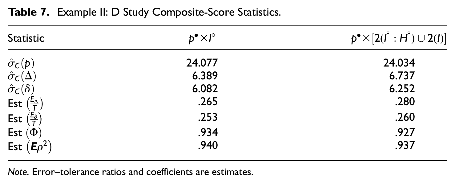
Table 7 provides estimates of composite standard deviations for universe scores, absolute errors, and relative errors, followed by error–tolerance ratios and coefficients. Results are provided for both the simplified $p^{•} \times I °$ design and the “actual“ $p^{•} \times [2 (I ° : H °) \cup 2 (I °)]$ design. For both designs, D study results are based on the G study sample sizes for items and testlets.

Table 7.

Example II: D Study Composite-Score Statistics.

Statistic	$p^{•} \times I °$	$p^{•} \times [2 (I^{°} : H^{°}) \cup 2 (I)]$
${\hat{σ}}_{C} (p)$	24.077	24.034
${\hat{σ}}_{C} (Δ)$	6.389	6.737
${\hat{σ}}_{C} (δ)$	6.082	6.252
Est $(\frac{E_{Δ}}{T})$	.265	.280
Est $(\frac{E_{δ}}{T})$	.253	.260
Est $(Φ)$	.934	.927
Est $(E ρ^{2})$	.940	.937

Note. Error–tolerance ratios and coefficients are estimates.

As expected, for both designs, relative error variance is consistently smaller than absolute error variance. Consequently, for both designs, $Δ$ -type error–tolerance ratios are larger than their $δ$ -type counterparts, and $Φ$ is smaller than $E ρ^{2}$ .

Basically, error–tolerance ratios quantify the magnitude of the SEM relative to the standard deviation of universe scores. As such, error–tolerance ratios are highly recommended because they are easy to interpret and they focus on SEMs, which are almost always the most important results of a D study analysis. By contrast, it is easy to exaggerate the meaningfulness of seemingly large coefficients. For example, for the actual $p^{•} \times [2 (I ° : H °) \cup 2 (I °)]$ design, $E_{Δ} / T$ is estimated to be .28, which means that the composite $Δ$ -type SEM is a little over 1/4 of the composite universe score standard deviation. In the authors’ experience, error–tolerance ratios of this magnitude are typically indicative of defensible measurement procedures, even though $E_{Δ} / T = . 28$ suggests that measurement error is not negligible. Mathematically, the estimated $Φ$ coefficient of approximately .93 captures the same information as $E_{Δ} / T = . 28$ , but the correlation-type metric (which involves variances) is more difficult to understand intuitively. Furthermore, $Φ = . 93$ appears so high (1 is perfection!) that it masks the fact that about ¼ of the standard deviation of universe scores is attributable to $Δ$ -type measurement error, which would not likely be judged negligible. As Cronbach (2004) stated,

Coefficients are a crude device that do not bring to the surface many subtleties implied by variance components. In particular, the interpretations being made in current assessments are best evaluated through use of a standard error of measurement. (p. 394)

It is reasonable to question whether $σ_{C} (Δ)$ or $σ_{C} (δ)$ is more relevant for making decisions about examinees. In general, $δ$ -type errors are more relevant when comparative scores (e.g., rank ordering) for examinees are the primary focus. By contrast, $Δ$ -type errors are relevant when decisions about examinees involve one or more cut scores. With AP, the authors believe absolute standard error, $σ_{C} (Δ)$ , is more important, but $σ_{C} (δ)$ might be relevant for some uses of AP scores.

At first glance, results for the $p^{•} \times I °$ design may appear remarkably similar to those for the actual design, but both $σ_{C} (Δ)$ and $σ_{C} (δ)$ are noticeably smaller for the $p^{•} \times I °$ design, which necessarily leads to lower error–tolerance ratios and higher coefficients. This does not mean that the $p^{•} \times I °$ design is better. Rather, the $p^{•} \times I °$ results appear better because they cover-up the impact of testlets in increasing measurement error. This impact can be noteworthy even when, as in this example, testlets affect only half of the complete test. Note, as well, that the impact of ignoring testlets is more pronounced for $Δ$ -based indices because they involve more error components that are affected by testlets (i.e., effects that include $h$ ).

Summary and Discussion

Univariate G theory can accommodate one or more fixed facets in certain restricted senses, but MGT does so in a much more elegant and flexible manner. Furthermore, estimation of variance components is often more complicated for a typical univariate G theory mixed model than for its MGT counterpart. In short, univariate G theory with a fixed facet is considerably more restrictive than MGT, especially the extension of MGT discussed in this article.

Brennan (2010) stated that “multivariate G theory is the whole of G theory, with univariate G theory simply being a special case” (p. 15). Still, virtually all prior MGT literature is limited in that it uses the same design structure for each level of a fixed facet. By contrast, this article has extended MGT largely through the explicit introduction of different designs for different levels of the fixed facet. Doing so permits a much more faithful analysis of the actual design structure of many tests, as illustrated by the mixed-format and testlets examples. This article also illustrates the use of error–tolerance ratios and advocates their use over coefficients, arguing that the former are much more easily and meaningfully interpreted than the latter.

The two examples in this article are particularly instructive in illustrating that (a) real-data applications are often much more complicated than is typically reflected by simplified analyses in much of the extant literature, (b) extended MGT is a viable alternative for such complex real-world measurement situations, (c) simplified analyses that do not capture real-data complexities often overstate measurement precision (see the testlets example), and (d) simplified analyses often hide important considerations about confounded facets (see the discussion of item-rater confounding in the mixed-format example).

It is recognized, of course, that real-world datasets may be limited in such a way that the types of analyses discussed in this article are not viable, and/or other practical circumstances may preclude performing the types of complex MGT analyses discussed here. Even so, it is almost always possible to describe a complex measurement procedure at a sufficient level of detail such that reported analyses can be qualified in a reasonable manner. Unfortunately, that is often not done. A particularly egregious example is the too frequent unqualified use of coefficient alpha as a presumably “adequate” reliability analysis. As Cronbach (2004) stated in his last published paper,

I no longer regard the alpha formula as the most appropriate way to examine most data. Over the years, my associates and I developed the complex generalizability (G) theory. (p. 403)

Some limitations of the present study should be noted. First, sample sizes (especially, numbers of raters) were small for Example I, which occasionally led to negative estimates of variance components, which were simply set to zero. This is not a practical problem in most large-scale testing programs in which raters are well-trained and, therefore, usually do not contribute much to the variability in observed scores (Brennan, 2000; Brennan & Johnson, 1995). Of course, analyses with larger number of raters would give improved estimates.

Second, the same single AP exam was used for both examples. Although the two examples were conducted with different sets of data, the use of the same exam might weaken the generalizability of the findings to other large-scale assessments that employ a format similar to AP German. Future research could be conducted using different tests to examine how generalizable results are to other similarly structured large-scale exams.

Third, the D studies reported here could be conducted with varying numbers of conditions. For example, the numbers of testlets and/or items could be manipulated for Example II to investigate the likely psychometric properties of a shortened or lengthened test.

Fourth, the 0 to 130 composite scores considered here for the two examples are indeed actual scores used with AP German. However, the scores reported to examinees are 1 to 5 integers. In principle, composite-score analyses could be conducted for the 1 to 5 scale. If that were done, additional analyses involving decision consistency likely would be appropriate, as well.

Finally, GENOVA and mGENOVA (which were used for the analyses in this article) employ the analogous ANOVA procedure to obtain estimated variance components. Alternatively, maximum likelihood and/or Bayesian procedures might be employed. In recent years, restricted maximum likelihood (REML) has become quite popular (see, for example, Jiang, 2018) especially as it precludes the possibility of obtaining negative estimates. Bayesian procedures are an even more flexible alternative (see, for example, Jiang & Skorupski, 2018; LoPilato et al., 2015). It should be recognized, however, that maximum likelihood and Bayesian procedures are computationally intensive and make normality assumptions that may be problematic.

Footnotes

Acknowledgements

The authors thank the College Board for making available the Advanced Placement data used in this paper.

Declaration of Conflicting Interests

The authors declared no potential conflicts of interest with respect to the research, authorship, and/or publication of this article.

Funding

The authors received no financial support for the research, authorship, and/or publication of this article.

ORCID iD

Stella Y. Kim

Notes

References

Brennan

R. L.

(2000). Performance assessments from the perspective of generalizability theory. Applied Psychological Measurement, 24, 339–353.

Brennan

R. L.

(2001a). Generalizability theory. Springer-Verlag.

Brennan

R. L.

(2001b). mGENOVA [Computer software and manual]. Center for Advanced Studies in Measurement and Assessment, The University of Iowa. https://education.uiowa.edu/research-centers/center-advanced-studies-measurement-and-assessment/computer-programs#GENOVA

Brennan

R. L.

(2010). Generalizability theory and classical test theory. Applied Measurement in Education, 24(1), 1–21.

Brennan

R. L.

(2016a). Weights in multivariate generalizability theory (CASMA Research Report No. 50). Center for Advanced Studies in Measurement and Assessment, The University of Iowa. https://education.uiowa.edu/sites/education.uiowa.edu/files/documents/centers/casma/publications/casma-research-report-50.pdf

Brennan

R. L.

(2016b). Using G theory to examine confounded effects: “The problem of one” (CASMA Research Report No. 51). Center for Advanced Studies in Measurement and Assessment, The University of Iowa. https://education.uiowa.edu/sites/education.uiowa.edu/files/documents/centers/casma/publications/casma-research-report-51.pdf

Brennan

R. L.

(2022). Generalizability theory. In Clauser

B. E.

Bunch

M. B.

(Eds.), The history of educational measurement (pp. 206–231). Routledge.

Brennan

R. L.

Johnson

E. G.

(1995). Generalizability of performance assessments. Educational Measurement: Issues and Practice, 14, 9–12.

College Board. (2019). AP classroom in here. https://apcentral.collegeboard.org/

10.

Crick

J. E.

Brennan

R. L.

(1983). GENOVA [Computer software and manual]. Center for Advanced Studies in Measurement and Assessment, The University of Iowa. http://www.education.uiowa.edu/casma

11.

Cronbach

L. J.

(2004). My current thoughts on coefficient alpha and successor procedures [Editorial assistance provided by R. Shavelson]. Educational and Psychological Measurement, 64, 391–418.

12.

Cronbach

L. J.

Gleser

G. C.

Nanda

Rajaratnam

(1972). The dependability of behavioral measurements: Theory of generalizability for scores and profiles. John Wiley.

13.

Jarjoura

Brennan

R. L.

(1982). A variance components model for measurement procedures associated with a table of specifications. Applied Psychological Measurement, 6(2), 161–171.

14.

Jarjoura

Brennan

R. L.

(1983). Multivariate generalizability models for tests developed according to a table of specifications. In Fyans

L. J.

(Ed.), New directions for testing and measurement: Generalizability theory (No. 18, pp. 83–101). Jossey-Bass.

15.

Jiang

(2018). Using the linear mixed-effect model framework to estimate generalizability variance components in R: A lme4 package application. Methodology, 14, 133–142.

16.

Jiang

Skorupski

(2018). A Bayesian approach to estimating variance components within a multivariate generalizability theory framework. Behavioral Research, 50, 2193–2214.

17.

Kane

M. T.

(1996). The precision of measurements. Applied Measurement in Education, 9, 355–379.

18.

Lee

(2000a). A comparison of methods of estimating conditional standard errors of measurement for testlet-based test scores using simulation techniques. Journal of Educational Measurement, 37, 91–112.

19.

Lee

(2000b). Estimating conditional standard errors of measurement for tests composed of testlets. Applied Measurement in Education, 13, 161–180.

20.

Lee

Frisbie

D. A.

(1999). Estimating reliability under a generalizability theory model for test scores composed of testlets. Applied Measurement in Education, 12, 237–255.

21.

LoPilato

A. C.

Carter

N. T.

Wang

(2015). Updating generalizability theory in management research: Bayesian estimation of variance components. Journal of Management, 41, 692–717.

22.

Moses

Kim

(2015). Methods for evaluating composite reliability, classification consistency, and classification accuracy for mixed-format licensure tests. Applied Psychological Measurement, 39, 314–329.

23.

National Center for Education Statistics. (2019). About NAEP. https://nces.ed.gov/nationsreportcard/about/

24.

Powers

Brennan

R. L.

(2009). Multivariate generalizability analyses of mixed-format advanced placement exams (Research Report No. 29). Center for Advanced Studies in Measurement and Assessment, The University of Iowa.

25.

Shavelson

R. J.

Webb

N. M.

(1991). Generalizability theory: A primer. SAGE.

26.

Sireci

S. G.

Thissen

Wainer

(1991). On the reliability of testlet-based tests. Journal of Educational Measurement, 28, 237–247.

Extended Multivariate Generalizability Theory With Complex Design Structures

Abstract

Keywords

An Overview of G Theory and MGT

Simple Univariate Example

Simple Multivariate Example

Composite Scores in MGT

Example I: Mixed-Format Tests

AP German Language Exam

Universe of Admissible Observations and Associated G Studies

G Study Designs

p • × i ° Design

p • × [ i ° ∪ ( i ° × r ° ) ] Design

p • × [ i ° ∪ ( r ° : i ° ) ] Design

Data

p • × i ° Design

p • × [ i ° ∪ ( i ° × r ° ) ] Design

p • × [ i ° ∪ ( r ° : i ° ) ] Design

Estimated G and D Study Variance and Covariance Components

Composite Summary Statistics

Example II: Tests With Testlets

Exam and Dataset

Universe of Admissible Observations

G Study p • × i ° Design

G Study p • × [ 2 ( i ° : h ° ) ∪ 2 ( i ° ) ] Design

D Study Results for Sections

D Study Results for Composite

Summary and Discussion

Footnotes

Acknowledgements

Declaration of Conflicting Interests

Funding

ORCID iD

Notes

References

$p^{•} \times i^{°}$ Design

$p^{•} \times [i ° \cup (i ° \times r °)]$ Design

$p^{•} \times [i ° \cup (r ° : i °)]$ Design

$p^{•} \times i^{°}$ Design

$p^{•} \times [i ° \cup (i ° \times r °)]$ Design

$p^{•} \times [i ° \cup (r ° : i °)]$ Design

G Study $p^{•} \times i^{°}$ Design

G Study $p^{•} \times [2 (i ° : h °) \cup 2 (i °)]$ Design