
Abstract
Prior research has shown that teachers receive lower pay compared to people with the same educational level who work in other occupations. This article challenges that literature and shows that by applying novel statistical approaches, the pay differentials are reduced, and even become pay premiums. In particular, these approaches provide unifying estimates that turn an earnings penalty between female teachers and non-teachers of approximately 10%—based on a standard approach in the literature—into an earnings premium of 5 to 10%. Likewise, estimates based on these approaches erase up to two-thirds of the earnings gap between male teachers and non-teachers. Moreover, going beyond the traditional focus on the mean, the author decomposes the pay gap across the entire earnings distribution. Estimates show that although teachers have a substantial earnings premium at the bottom of the distribution, they have a large earnings penalty at the top.
An enduring debate in public education is whether school teachers are adequately compensated, since teachers are critical to children’s achievements and, consequently, an important determinant of their long-term educational and labor market outcomes. 1 In the United States, teachers’ wages are set by state or school district decree, legislative fiat, and collective bargaining. Federal, state, and local government funding determines school districts’ ability to compensate teachers. Increased budget constraints on the part of states and school districts, along with the rigid wage schedule, has made the long-standing question of pay in the teachers’ labor market more relevant: How are teachers paid relative to similar workers in other sectors?
Understanding the pay gap is important for compensation planning and management, as these factors can presumably lead to big efficiency gains to schools (Podgursky 2011). 2 Studies have shown that teachers earn less than non-teachers with similar observable skills (Taylor 2008; Allegretto and Mishel 2016). Further, as studies in the literature have attempted to connect teachers’ relative pay, their quality (Hanushek and Rivkin 1997; Stoddard 2003), and their labor supply, credible and comprehensive estimates of the pay gap facilitate a more nuanced view of the connection. 3
A critical challenge in analyzing teacher pay is the lack of a directly comparable group of non-teachers to recover teachers’ counterfactual earnings because teachers and non-teachers are not randomly assigned. I use three main empirical approaches not considered previously to tackle various potential biases and to document systematically new and robust empirical facts about the earnings gap.
First, I control for field-of-study fixed effects in the standard Mincer regression to erase a bias arising from individuals’ career preferences, aspirations, and, to some extent, abilities. To do so, I leverage newly available data on field of study from the American Community Survey (ACS), covering 2009 to 2017. Second, I address omitted variable bias stemming from the differential pay for the variable nature of job characteristics by controlling for measures of a given occupation’s task contents. Occupations differ in terms of the content of tasks involved, leading to differential compensation. Following Autor and Dorn (2013), I use three broader measures of tasks at the 3-digit occupation level: abstract, routine, and manual. Third, I employ a propensity score matching (PSM) strategy to disentangle the relative earnings of teachers from observable differences in their characteristics. I match teachers with non-teachers based on their demographic characteristics, time and geographic fixed effects, and field of study.
All of these approaches provide similar trends and suggest that female teachers earn approximately 5 to 10% more than comparable non-teachers earn. This result is contrary to the finding of approximately 10% lower earnings for female teachers based on a standard Mincer regression, which is commonly adopted in the teacher pay literature. Similarly, the three approaches I follow erase up to two-thirds of the earnings gap between male teachers and non-teachers.
To provide further insights into earnings differences, I next move beyond the traditional focus on the mean to examine earnings gaps across the entire distribution. The average pay gap is at the center of policy debates on teacher pay, yet it misses important pay gap patterns that complicate the problem regarding teacher compensation structures and hinder school districts’ ability to identify potential policies to address the problem. Given the compressed and rigid nature of teachers’ salary schedule, their pay is a manner of “high-floor and low-ceiling.” A high floor leads to a situation in which a teacher at the lower part of the distribution is potentially paid higher than an otherwise similar non-teacher, resulting in a substantial unexplained differential for teachers’ earnings. Conversely, a low-ceiling pay structure prevents teachers from being adequately compensated at the top of the distribution.
I apply a quantile decomposition approach based on the recentered influence function (RIF) and provide the first empirical evidence of earnings differences beyond the mean and the potential sources behind such differences in the teachers’ labor market. I partition the earnings gap at a given percentile into 1) a component that is explained by individual or group characteristics (i.e., explained gap) and 2) a component that reflects differential wage schedules across the two sectors (i.e., unexplained gap). My results reveal noteworthy patterns in heterogeneous returns to teachers. Although many teachers enjoy a significant earnings premium at the lower end of the distribution, others face a substantial earnings penalty at the top.
Relation to Existing Work
This article contributes to, and connects with, several strands of the existing literature. First, it substantially improves a long literature that analyzes the relative wages of teachers. The findings reach a consensus of a decline in teacher pay (see Podgursky and Springer 2011 and Podgursky 2011 for review). The most recent studies show the earnings gap between teachers and non-teachers in the range of around 7 to 14% (Taylor 2008; West 2014; Allegretto and Mishel 2016). West (2014) provided new insight into teacher pay by controlling for the number of hours worked per week with time-use diary data from the American Time Use Survey (ATUS). The author found that teachers work, on average, 34.5 hours per week annually as compared to 39.8 hours per week worked by non-teachers, and that based on estimated hours of work, high school teachers earn 7 to 14% less than non-teachers earn. Taylor (2008) used Public Use Microdata Areas (PUMA) fixed effects to account for the geographical sorting between teachers and non-teachers, given that teachers are located in all parts of the country and non-teachers tend to be located in cities. She found that teachers earn approximately 8% less than do non-teachers. Using Current Population Survey (CPS) data, Allegretto and Mishel (2016) documented the weekly wage gap between teachers and non-teachers on an annual basis. The wage penalty for female teachers was 7.7% in 2009 and 13.9% in 2015, the latest year of their analysis. Richwine and Biggs (2011) offered an initial analysis of the wage gap between teachers and non-teachers using the Survey of Income and Program Participation (SIPP) panel data. In a related study, Schanzenbach (2015) re-examined the public-sector pay gap using Armed Forces Qualification Test (AFQT) results and college majors. The author found that individuals with lower skills select into the public sector and that the public-sector pay gap decreases considerably after controlling for fields of study.
By virtue of using the measures of task contents of occupations, this article contributes to a growing body of work that examines how tasks affect the wage distribution. Using a British survey, Fernández and Nordman (2009) found that job attributes such as “repetitive,”“requiring literacy skills,” and “requiring customer handling skills” become a substantial source of wage differentials across jobs, creating wage premiums and penalties. Likewise, Autor, Levy, and Murnane (2003), Acemoglu and Autor (2011), and Deming (2017) explored the importance of various skills or tasks in explaining wage inequalities across groups in the labor market.
This article is connected to others in the literature that also use PSM to explain the wage gap. For example, Mizala, Romaguera, and Gallegos (2011) applied the matching approach to explain the public–private wage gap in Latin America. Frölich (2007) employed this approach to investigate the gender wage gap among graduates in the United Kingdom. Ñopo (2008) explained the methodology of a matching approach for investigating wage differences across genders.
Another feature of this study is the quantile decomposition technique based on RIF regressions to understand the earnings gap between teachers and non-teachers across the entire distribution. In being the first study to apply the decomposition approach in the context of the earnings gap between teachers and non-teachers, this article is related to an emerging literature that employs this approach to evaluate the distributional effects of public policies (Aaberge, Bhuller, Langørgen, and Mogstad 2010; Dube 2019) and the gender wage gap. Kassenboehmer and Sinning (2014) applied this approach to explain the gender wage gap in the United States, while Bhalotra and Fernandez (2018) used it to illustrate the role of women’s labor force participation in the gender wage gap.
To summarize, two broader contributions of the present study stand out. First, it offers new, robust empirical facts about the relative earnings of teachers by being the first to control for college major fixed effects and for task contents of occupations and being the first to use a matching approach. Since each strategy has its own advantages in improving the direct comparison between teachers’ and non-teachers’ baseline characteristics or content of work, their collective use should combat varying potential biases and produce more credible estimates. Second, my study offers the first investigation into the earnings gap across the entire distribution, using a quantile decomposition.
Data
American Community Survey
I use data from the 2009 to 2017 ACS extracted from the Integrated Public Use Microdata Series (Ruggles et al. 2019). The ACS samples 1% of the total population in the United States. Note that the ACS has been reporting the chosen fields of study for individuals pursuing bachelor’s degrees only since 2009. I restrict the sample to prime-age working people, ages 25 to 54. I exclude those below 25 years to avoid the issues related to youth unemployment and early career choices and exclude those above 54 years to avoid retirement issues. As the teaching profession requires at least a four-year college degree, I limit the sample to those having a bachelor’s degree or beyond. Additionally, I exclude self-employed, unemployed, unpaid family workers, and those in the armed forces.
The ACS reports an individual’s pre-tax salary income received from an employer during the past 12 months. I deflate annual incomes to 2009 dollars. As Bollinger and Hirsch (2006) showed that earnings imputation in household surveys biases estimates, I exclude those individuals whose earnings are imputed. Similarly, the survey provides information on a respondent’s number of weeks worked during that period in intervals, such as 1 to 13 weeks, 14 to 26 weeks, 27 to 39 weeks, and 40 to 52 weeks. I drop respondents who have missing values for the number of weeks worked or have zero income, which could also reflect their non-working status during the period.
To define teachers and non-teachers, I use the variable “OCC1990,” which derives from the 1990 Census Bureau occupational classification scheme. I classify individuals into the “teachers” group if they report being kindergarten and earlier school teachers, primary school teachers, secondary school teachers, or special education teachers. 4 I exclude private school teachers because their compensation mechanisms and working environments differ from those of public school teachers. I also drop those who report their occupation as “teachers not mentioned elsewhere,” as it is not obvious if they are full-time, regular school teachers or represent non-school teachers such as private tutors.
Table 1, panel A, reports descriptive statistics for female teachers and non-teachers; Table 2, panel A, presents the same information for male teachers and non-teachers. The raw income is lower for teachers than for non-teachers. Another notable difference is observed for the variable “master’s degree.” Approximately 52% of female and 51% of male teachers have a master’s degree, whereas approximately 25% of female and male non-teachers have such a degree. Compared to non-teachers, teachers are more likely to have been married and to have a greater number of children.
Summary Statistics for Women
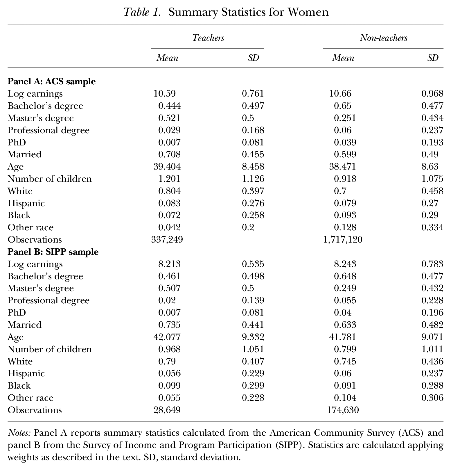
Notes: Panel A reports summary statistics calculated from the American Community Survey (ACS) and panel B from the Survey of Income and Program Participation (SIPP). Statistics are calculated applying weights as described in the text. SD, standard deviation.
Summary Statistics for Men
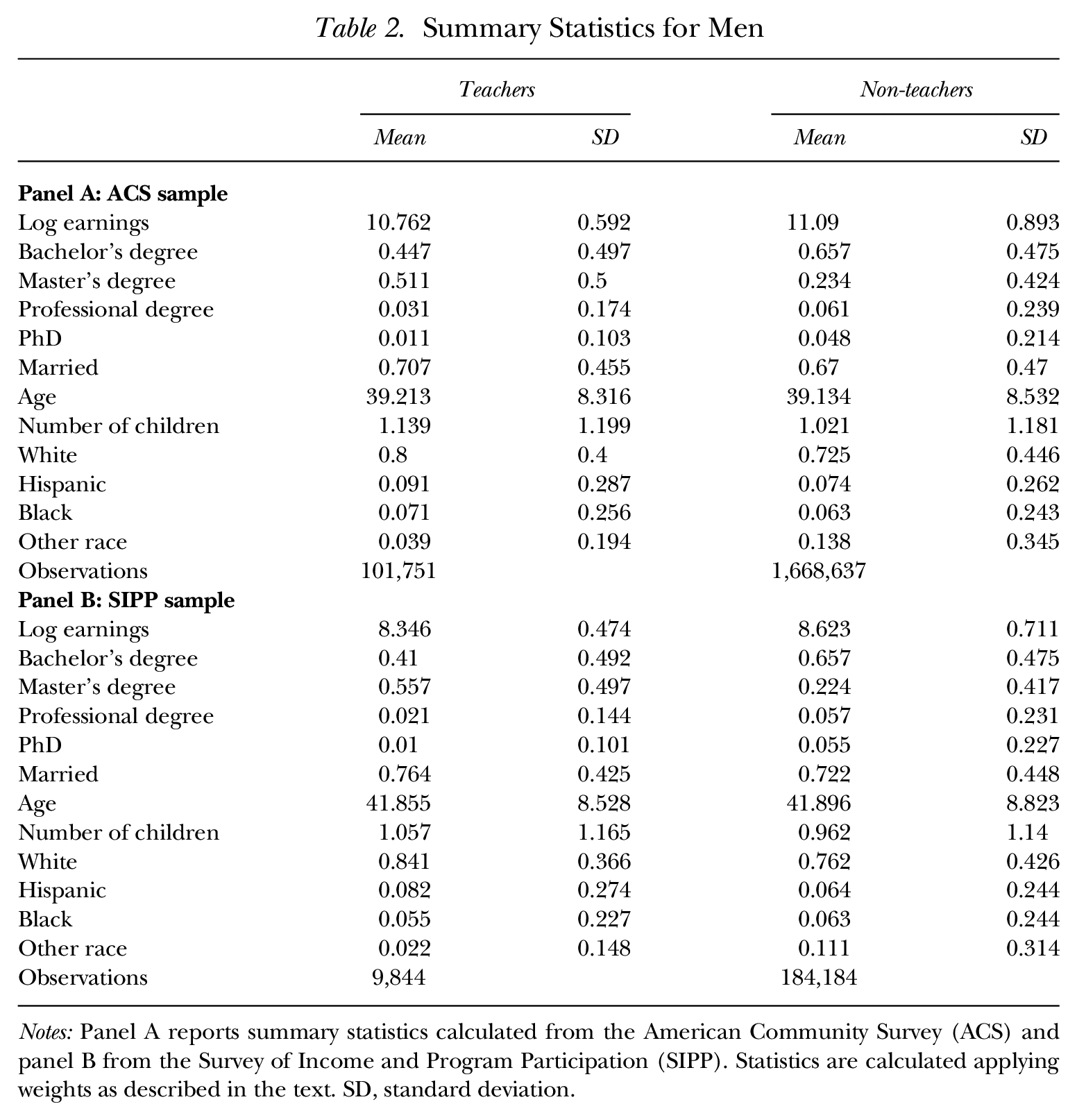
Notes: Panel A reports summary statistics calculated from the American Community Survey (ACS) and panel B from the Survey of Income and Program Participation (SIPP). Statistics are calculated applying weights as described in the text. SD, standard deviation.
Survey of Income and Program Participation
I use the 2008 Survey of Income and Program Participation (SIPP) panel, which overlaps the time frame of the ACS. This particular panel of the nationally representative longitudinal survey lasted from 2008 to 2013. I define teachers in the SIPP in a manner similar to that of the ACS. I drop family workers and non-workers (those whose occupation is missing). As in the ACS data, I restrict the sample to those who were at least 25 years of age at the beginning of the survey and did not exceed 54 years of age throughout the sample. Income refers to monthly earnings from an individual’s job. 5 Table 1, panel B reports descriptive statistics for female teachers and non-teachers and Table 2, panel B for male teachers and non-teachers. Both tables show patterns qualitatively similar to those from the ACS. Note that the SIPP measures income on a monthly basis whereas the ACS reports annual income. This difference explains the visible discrepancy between the ACS and SIPP data in terms of income.
Empirical Estimations and Results
Baseline Estimation and Results
I first use the standard Mincer regression to examine the pay difference between teachers and non-teachers. In particular, I estimate the regression model of the following form:

where
One potential issue of using this standard model to calculate the relative earnings of teachers is its inability to disentangle the earnings gap from the cost of living. Taylor (2008) argued that unlike college-educated workers in the non-teaching sector, teachers tend to be scattered across the state, including in rural areas, and failure to control for labor market areas biases the relative wage estimates. Taylor (2008) used PUMA fixed effects. PUMAs are geographic units, each containing at least 100,000 persons, within a state; however, the areas are not delineated to reflect similar labor markets or economic characteristics. Therefore, they may not be a good measure of the cost of living.
To better control for the cost of living, I compare teachers and non-teachers in the same labor market, defined as the commuting zone (CZ). The CZ is defined on the basis of journey-to-work data and includes counties having similar labor market conditions. Approximately 740 CZs exist across the United States. They can extend across state borders.
Using population data from the most recent decennial census, the Census Bureau changes the PUMA boundaries every 10 years. To map PUMAs to CZs for the ACS samples from 2009 to 2011, which are based on the 2000 Census, I use a crosswalk following Autor and Dorn (2013). For the ACS samples from 2012 to 2017, which are based on the 2010 Census, I use a crosswalk following Autor, Dorn, and Hanson (2019).
PUMAs can include a county or a cluster of counties. Most of the PUMAs are matched to unique CZs. Some PUMAs, however, extend across multiple counties that fall into multiple CZs, which means that PUMAs may be mapped into more than one CZ. For individuals from such PUMAs, I recalculate their census weights by a new measure that is the proportional probability of each individual from each PUMA belonging to a given CZ, as in Autor and Dorn (2013).
Baseline Estimates
I begin by reporting the results based on Equation (1). Table 3, panel A, contains the results for women. As shown in column (1), I find that female teachers are paid 100 × (
Relative Earnings of Teachers
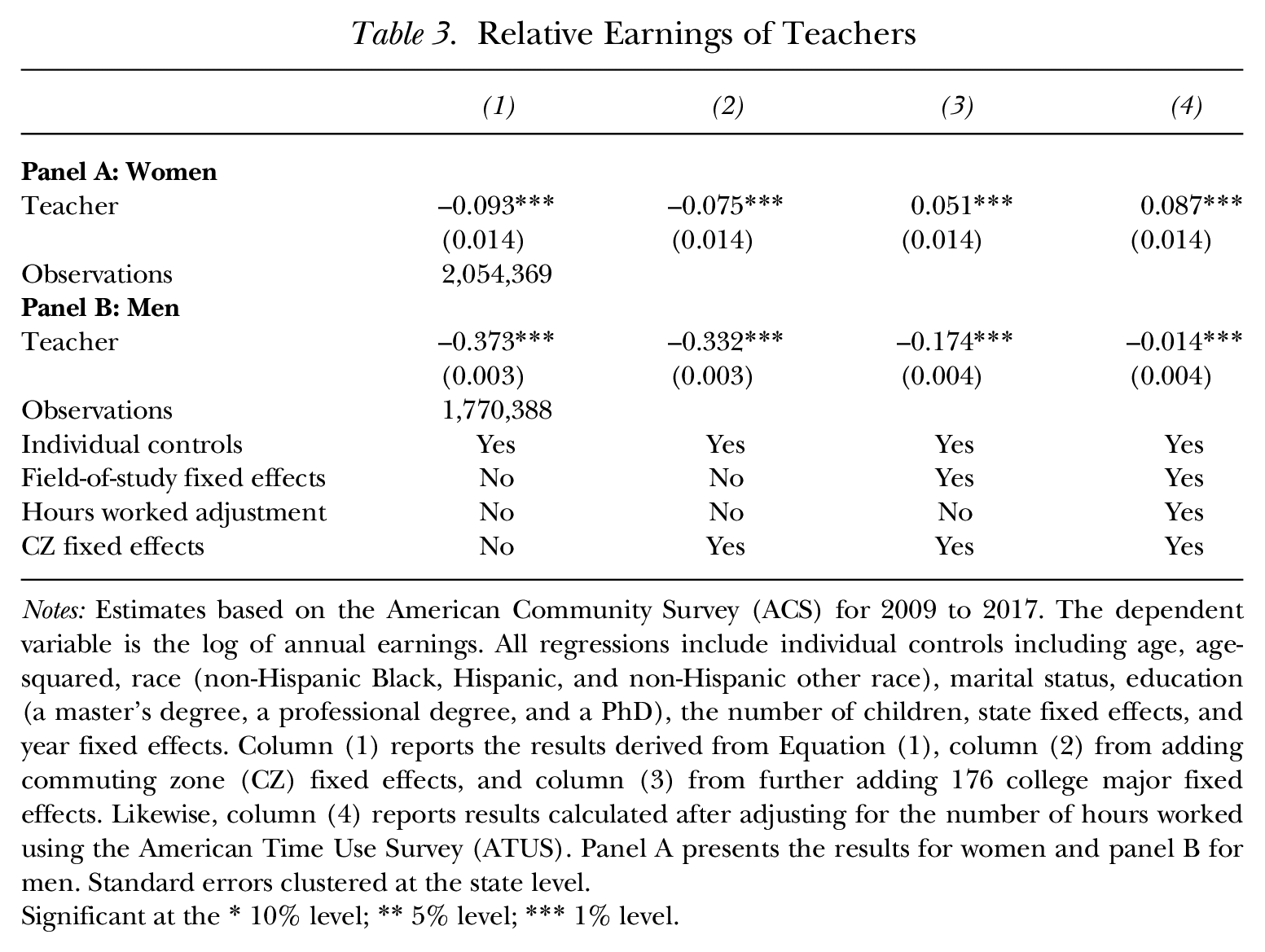
Notes: Estimates based on the American Community Survey (ACS) for 2009 to 2017. The dependent variable is the log of annual earnings. All regressions include individual controls including age, age-squared, race (non-Hispanic Black, Hispanic, and non-Hispanic other race), marital status, education (a master’s degree, a professional degree, and a PhD), the number of children, state fixed effects, and year fixed effects. Column (1) reports the results derived from Equation (1), column (2) from adding commuting zone (CZ) fixed effects, and column (3) from further adding 176 college major fixed effects. Likewise, column (4) reports results calculated after adjusting for the number of hours worked using the American Time Use Survey (ATUS). Panel A presents the results for women and panel B for men. Standard errors clustered at the state level.
Significant at the * 10% level; ** 5% level; *** 1% level.
Next, I estimate the earnings gap between male teachers and non-teachers. As reported in Table 3, panel B, the results from the standard Mincer regression show that the earnings of male teachers are approximately 45% lower than the earnings of male non-teachers (column (1)). When I control for CZ fixed effects, the earnings gap falls to approximately 39% (column (2)).
Importance of College Majors
College major choice is an important factor underlying earnings differences. Such choice could reflect the ability-based sorting of individuals (Arcidiacono 2004) or preferences for a particular occupation based on non-pecuniary returns (see Altonji, Blom, and Meghir 2012 for a review). Figure 1 presents the association between the proportion of individuals who become teachers by their field of study and the relative pay of teachers in that field. Heterogeneous returns to the field of study raise the importance of controlling for college majors to account for the self-selection of individuals into occupations. 7 Therefore, I further add college major fixed effects. I consider 176 fields of study in which individuals obtain their bachelor’s degrees. As reported in Table 3, I find that for women, the earnings of teachers are 5.2% higher than those of similar non-teachers (panel A, column (3)). For men, when I add field-of-study fixed effects, the earnings gap falls to 19% (panel B, column (3)). Additionally, I examine the wage profiles of teachers and find that the return to experience is lower in teaching than in non-teaching jobs. 8
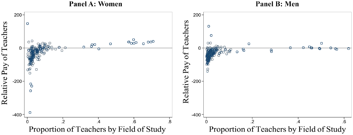
Relative Teacher Pay and Proportion of Teachers by Field of Study
In this analysis, I compare teachers and non-teachers who hold a degree in the same field of study but pursue careers in different sectors (teaching versus non-teaching). The estimates are obtained under the assumption that individuals majoring in the same field of study have a similar set of skills and talents. A potential concern, however, is that those who choose a similar college major but embark on dissimilar career paths may have different underlying characteristics and backgrounds. For example, it is possible that those who major in education but do not become teachers were not successful in teaching or that they have underlying abilities and career preferences that differ from those who become teachers.
Work hours.
A key discussion in the teacher pay literature focuses on whether teachers tend to work shorter hours. The problem with the survey data in measuring work hours is that workers tend to overstate their work hours (West 2014). Therefore, I turn to the ATUS, which uses time-use diaries of individuals. Analyzing these diaries from 2009 to 2017, I find that female teachers work approximately 34.16 hours per week, compared to 35.34 hours worked per week by non-teachers. 9 I re-estimate Equation (1), adjusting for weekly hours worked. To do so, I first calculate the average annual work hours for each group by multiplying average weekly work hours by 52. Then, I divide the earnings of each individual in each sector by the respective average annual work hours. The pay premium for female teachers increases to 9% (Table 3, column (4)). I find a large difference in the number of hours worked per week between male teachers and non-teachers. Male teachers work 36.5 hours per week, whereas male non-teachers work 42.6 hours per week. When I adjust this discrepancy in hours worked, the earnings gap declines to approximately 1.9% (Table 3, column (4)). Though these estimates are illustrative of a general pattern of pay differences related to work hours, a caveat is that these values are derived by extrapolating the annual number of hours worked. 10
Heterogeneous returns.
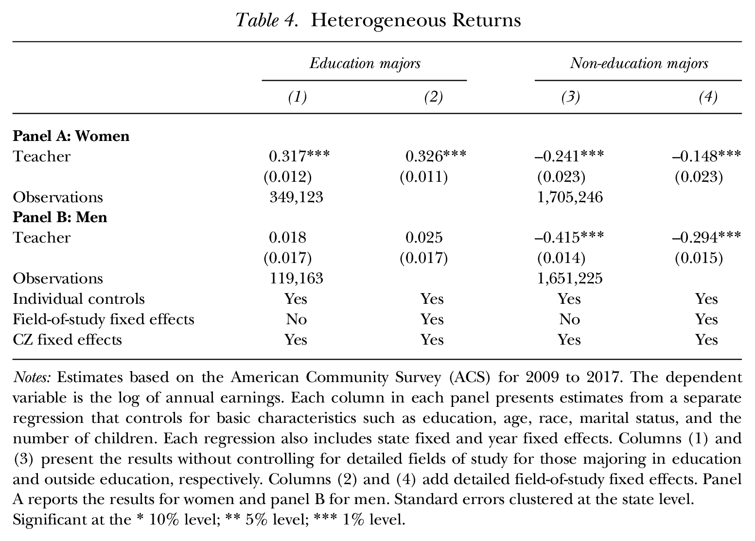
Considering that teachers typically tend to be drawn from among individuals majoring in the field of education (see Tables OA.1 and OA.2 in the Online Appendix), analysis of the pay gap experienced by those with and without having majored in education can provide more nuanced insights. 11 Because a major in education is a conventional route to a teaching career, education majors can reflect self-selection of aspiring educators into teaching. Therefore, I separately estimate the pay differences for these two groups: education and non-education majors.
Table 4 contains these results. Columns (1) and (3) present the results without controlling for detailed fields of study for those majoring in education and outside education, respectively. Columns (2) and (4) add detailed field-of-study fixed effects. As shown in panel A, female teachers who majored in education earn approximately 38.5% more than female non-teachers who majored in education. However, the results reveal what amounts to a penalty in pay of approximately 15.9% for female teachers who hold non-education degrees as compared to those non-teachers who hold non-education degrees. Likewise, male teachers majoring in education do not face any pay penalty. Male teachers who did not pursue education majors earn approximately 34.1% less than do similar non-teachers. Overall, this analysis provides insight into pay differentials, indicating the potential self-selection of individuals into majoring in education and subsequently becoming teachers.
Heterogeneous Returns
Notes: Estimates based on the American Community Survey (ACS) for 2009 to 2017. The dependent variable is the log of annual earnings. Each column in each panel presents estimates from a separate regression that controls for basic characteristics such as education, age, race, marital status, and the number of children. Each regression also includes state fixed and year fixed effects. Columns (1) and (3) present the results without controlling for detailed fields of study for those majoring in education and outside education, respectively. Columns (2) and (4) add detailed field-of-study fixed effects. Panel A reports the results for women and panel B for men. Standard errors clustered at the state level.
Significant at the * 10% level; ** 5% level; *** 1% level.
Importance of Occupational Tasks
As noted earlier, college majors account for omitted variables bias resulting from individuals’ ability and skills, which are homogenous among individuals within a field of study. Still, estimates may suffer from other potential biases arising from differential skill and work effort requirements across occupations. Some occupations involve carrying out repetitive tasks, while others require intense knowledge and analytical skills. This differential nature of occupations has natural implications for the salary in the teachers’ labor market. Teachers could be paid less because their job characteristics differ from those of other college graduates.
To tackle such biases and isolate the relative earnings of teachers, I add direct measures of various skills and work effort required in a particular job to the standard Mincer regression. I use the task measures, which help to characterize the type of work performed across occupations. An emerging literature uses this “task approach” to analyze earnings inequality (see Acemoglu and Autor 2011 and Autor 2013 for reviews). Using the task content measures in the analysis of the relative earnings of teachers seems relevant to derive more nuanced estimates. Following Autor and Dorn (2013), I use three broader measures of tasks for each occupation: abstract, routine, and manual. Autor and Dorn (2013) classified tasks into these three measures using the US Department of Labor’s Dictionary of Occupational Titles. These task contents are measured at the 3-digit occupation level. 12 The value of abstract measure ranges from 0 to 9, of routine measure from 1.19 to 8.65, and of manual measure from 0 to 10. 13
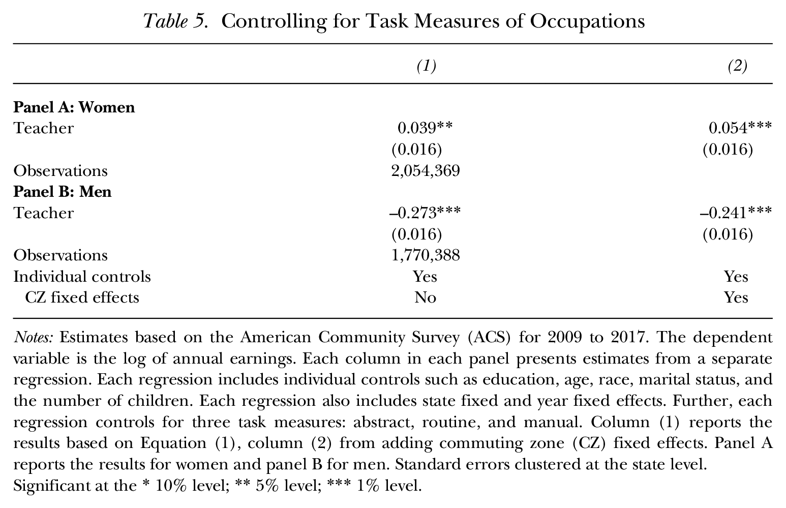
I re-estimate Equation (1) using controls for the three measures of task contents of occupations. The findings reveal patterns similar to those that emerged from a specification using field-of-study fixed effects. Table 5 contains the results. Column (1) reports findings without controlling for CZ fixed effects and column (2) adds controls for the CZ fixed effects. I find that female teachers are paid 4 to 5.5% more than female non-teachers are paid. Likewise, the controls of the task measures erase a substantial pay gap for male teachers.
Controlling for Task Measures of Occupations
Notes: Estimates based on the American Community Survey (ACS) for 2009 to 2017. The dependent variable is the log of annual earnings. Each column in each panel presents estimates from a separate regression. Each regression includes individual controls such as education, age, race, marital status, and the number of children. Each regression also includes state fixed and year fixed effects. Further, each regression controls for three task measures: abstract, routine, and manual. Column (1) reports the results based on Equation (1), column (2) from adding commuting zone (CZ) fixed effects. Panel A reports the results for women and panel B for men. Standard errors clustered at the state level.
Significant at the * 10% level; ** 5% level; *** 1% level.
Overall, this analysis improves the standard Mincer regression, which relies on basic characteristics such as education and experience for explaining the earnings differences, by incorporating occupation-specific task prices to the regression. In other words, I include previously omitted variables regarding the role that the returns to the measures of task content plays in the overall pay differences between the teaching and non-teaching sectors, thus more credibly isolating the relative earnings of teachers.
Conditioning on task content measures and basic demographic characteristics, along with time and location differences, the analysis assumes that the remaining earnings gap between teachers and non-teachers is attributable to differential wage structures across the two sectors. That these task measures can fully capture unobserved differences in skill sets and work requirements, and that task contents within an occupation are uniform, provide additional assumptions needed to address the problem of omitted variables bias arising from job characteristics. It is plausible, however, that job tasks within an occupation are heterogeneous, which can bias estimates. Likewise, task scores are calculated by mapping a large number of task contents provided by the Dictionary of Occupational Titles to broader measures for each occupation, which raises the possibility of measurement error. And, it is possible that other unmeasured contents of tasks specific to jobs influence pay.
Propensity Score Matching
Estimates of the earnings gap between teachers and non-teachers could be driven by imbalances in characteristics between teachers and non-teachers. As randomization is practically infeasible in the teachers’ labor market, the closest approach that can be adopted in my setting is propensity score matching (PSM). The PSM approach that is widely used in the treatment evaluation is equally relevant for analyzing wage differences between two groups (Ñopo 2008). Therefore, I use PSM as yet another strategy to erase a confounding effect that results from systematic differences in baseline characteristics between teachers and non-teachers.
To implement the PSM, I use a nearest-neighbor matching of a nonparametric nature and follow a newly developed procedure in calculating standard errors for the post-matched regression. I apply one-to-one matching without replacement, which matches each teacher to the most comparable non-teacher. The main advantages of this matching approach are transparency and straightforwardness.
To execute the process empirically, in the first step, I calculate the propensity score of being a teacher. The score represents the predicted probability derived from a logit model (Rosenbaum and Rubin 1985; Imbens 2004). I regress an indicator variable for teacher on demographic variables such as education, race, and children, fields-of-study fixed effects, state fixed effects, year fixed effects, and commuting zone fixed effects. Formally, I use the following model:

where
One issue in running the post-matched regression is how to correctly calculate standard errors that account for the uncertainty involved in the estimation of the propensity score in the first stage. The literature has widely used a bootstrap technique to address this problem. Abadie and Imbens (2008), however, explained that bootstrap standard errors are not generally valid. In a recent paper, Abadie and Spiess (2021) derived asymptotically valid standard errors in the post-matched regression based on nearest-neighbor matching without replacement. Note that since my study uses a nearest-neighbor matching strategy without replacement to match teachers and non-teachers, Abadie and Spiess (2021) is highly relevant in the context of this analysis. The authors show that the ordinary least squares (OLS) standard errors in the post-matched regression are valid as long as 1) matching is done without replacement and 2) the regression is correctly specified relative to the population regression. They also suggest using clustered standard errors at the matched-pair level when the post-matching regression is not correctly specified. I follow Abadie and Spiess (2021) and cluster standard errors at the matched-pair level.
Evidence from a Matching Approach
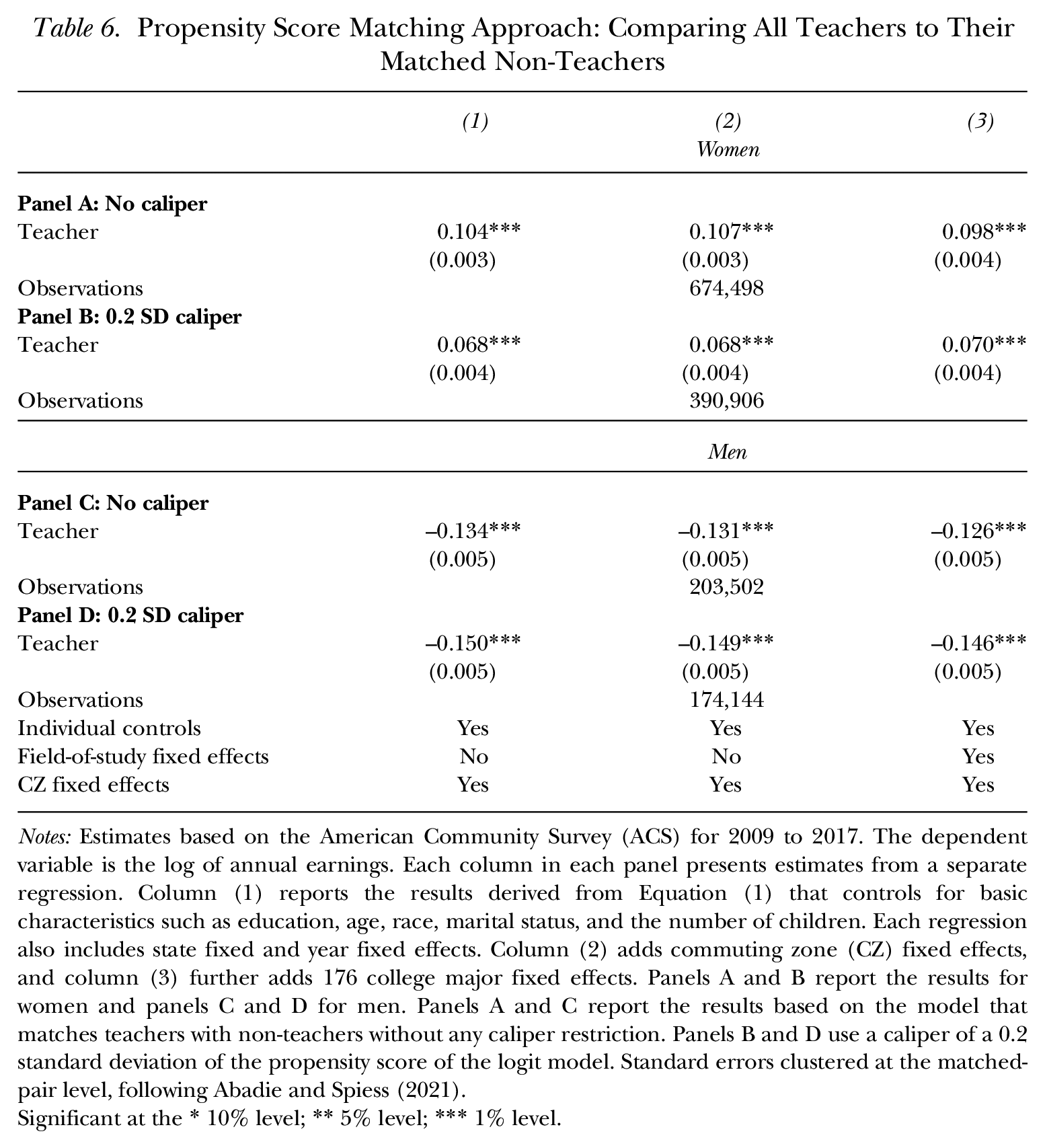
To make the estimation strategy simple, and for the purpose of illustration, I begin my analysis by matching each teacher to a non-teacher regardless of the closeness of the match. This approach permits me to retain all teachers in the sample. Therefore, the comparison group represents non-teachers who have similar characteristics as teachers. I report the results in Table 6. I estimate the three main baseline specifications. First, I use individual controls, year fixed effects, and state fixed effects. Second, I add CZ fixed effects. Finally, I further add field-of-study fixed effects. Across all three specifications, the results are similar. The robustness to additional controls highlights the quality of the match performed. In terms of magnitude, in my preferred specification, female teachers have approximately 10.2% higher earnings than female non-teachers have (panel A, column (3)). Likewise, for male teachers, the PSM technique lowers the gap to 13.4% (panel C, column (3)), accounting for more than two-thirds of the earnings gap witnessed in the baseline regression.
Propensity Score Matching Approach: Comparing All Teachers to Their Matched Non-Teachers
Notes: Estimates based on the American Community Survey (ACS) for 2009 to 2017. The dependent variable is the log of annual earnings. Each column in each panel presents estimates from a separate regression. Column (1) reports the results derived from Equation (1) that controls for basic characteristics such as education, age, race, marital status, and the number of children. Each regression also includes state fixed and year fixed effects. Column (2) adds commuting zone (CZ) fixed effects, and column (3) further adds 176 college major fixed effects. Panels A and B report the results for women and panels C and D for men. Panels A and C report the results based on the model that matches teachers with non-teachers without any caliper restriction. Panels B and D use a caliper of a 0.2 standard deviation of the propensity score of the logit model. Standard errors clustered at the matched-pair level, following Abadie and Spiess (2021).
Significant at the * 10% level; ** 5% level; *** 1% level.
Next, I match teachers and non-teachers within a specific caliper width, which is calculated as the difference in the propensity score of the matched pair. The literature offers no unanimous caliper width to adopt in the empirical analysis. Cochran and Rubin (1973) and Rosenbaum and Rubin (1985), however, suggested that a caliper width that is 0.2 of the standard deviation of the logit of the propensity score erases approximately 98% of bias resulting from the measured confounders. Therefore, I re-estimate the PSM approach using the suggested caliper width. I am able to match approximately 50% of female teachers and 90% of male teachers to their comparable non-teachers. Specifically, the treatment group here represents the teachers I am able to match with similar non-teachers (the comparison group). As shown in Table 6, panel B, column (3), female teachers earn approximately 7.2% more than non-teachers. Likewise, for male teachers, the pay gap stands at approximately 15.7% (panel D, column (3)), down from 45% found in the model based on Equation (1). 14
Note that my estimates are conditional on the identifying assumption that observable characteristics entirely explain individuals’ underlying ability or productivity determining their earnings. This approach selects a comparison group based on those observed characteristics only. It is possible that teachers and non-teachers differ in terms of other unobserved characteristics, which can influence earnings. Likewise, they might be choosing teaching and non-teaching jobs based on their underlying productivity, potentially violating the assumption.
Panel Data Approach
I make use of the panel data to employ an alternative approach to tackle a critical concern on whether omitted variables, such as fixed unobserved workers’ productivity, are contributing to the observed pay difference. I obtain the data from the 2008 panel of the Survey of Income and Program Participation (SIPP). Because this particular panel of the survey covers approximately five years, I can observe an individual’s occupation over time, as well as salary in both the teaching and non-teaching sectors if the person switches their occupation. I use the specification parallel to Equation (1), controlling for individual fixed effects.
In this specification,

where variables are defined as above, except that
Evidence from the Panel Data
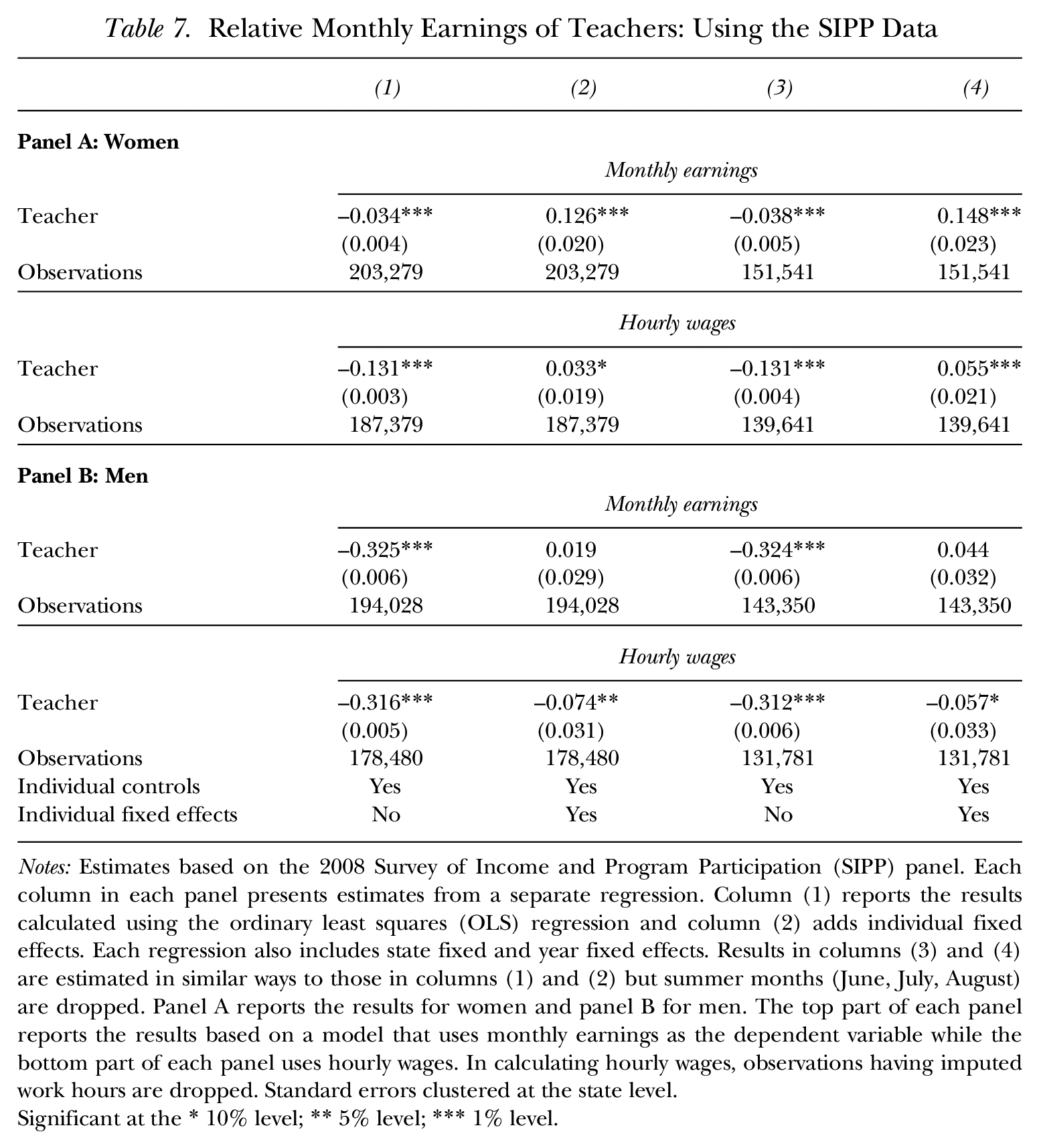
In this subsection, I present the results estimated using the panel data from the SIPP (see Table 7). I first estimate the effects of being a teacher on monthly earnings based on an OLS estimation using individual-level control variables and state fixed effects. As shown in column (1) at the top of panel A, female teachers are paid approximately 3.5% less than non-teachers. This estimate is smaller than the estimate from the ACS data, which could be because of sample variation. Next, I control for individual fixed effects, which turn a negative earnings gap into an earnings premium. Specifically, female teachers earn approximately 12.7% more than female non-teachers (column (2) at the top of panel A). One concern in this analysis is that it is possible for teachers to work in another occupation during the summer months when schools are off. To address such a concern, I drop the months of June, July, and August from my analysis and re-estimate Equation (3). Column (3) at the top of Table 7 presents the results derived without individual fixed effects, and column (4) controlling for individual fixed effects. Dropping summer months yields similar results. Because the SIPP reports the number of hours worked per month, I am able to calculate hourly earnings. 15 I re-estimate my models on hourly earnings. I estimate parallel models for men and present the results in panel B. Controlling for individual fixed effects erases most of the earnings penalty for male teachers.
Relative Monthly Earnings of Teachers: Using the SIPP Data
Notes: Estimates based on the 2008 Survey of Income and Program Participation (SIPP) panel. Each column in each panel presents estimates from a separate regression. Column (1) reports the results calculated using the ordinary least squares (OLS) regression and column (2) adds individual fixed effects. Each regression also includes state fixed and year fixed effects. Results in columns (3) and (4) are estimated in similar ways to those in columns (1) and (2) but summer months (June, July, August) are dropped. Panel A reports the results for women and panel B for men. The top part of each panel reports the results based on a model that uses monthly earnings as the dependent variable while the bottom part of each panel uses hourly wages. In calculating hourly wages, observations having imputed work hours are dropped. Standard errors clustered at the state level.
Significant at the * 10% level; ** 5% level; *** 1% level.
Although the panel data are helpful to purge unmeasured individual heterogeneities in the pay gap analysis, it is important to keep a drawback in mind while interpreting the results. Individuals who move into and out of teaching include a small subset who may be self-selecting into occupations based on the suitability of their skills (Scafidi, Sjoquist, and Stinebrickner 2006). Their decision to switch jobs may be driven by various life events, such as marriage, health, children, spousal labor supply, and location preferences. A pursuit for an optimum labor–leisure choice or preferences for certain types of work in terms of predictability and stability may also motivate individuals to change their careers. If such underlying factors are driving their move in and out of teaching, the results here are biased.
Quantile Decomposition of the Earnings Gap
So far, as in the literature, this analysis focuses on the pay gap at the mean only. To provide further insights into earnings differences, I move beyond the mean to look at earnings gaps across the entire distribution. This analysis is highly relevant because of the implications of the “low-ceiling-and-high-floor” nature of the wage schedules prevailing in the teaching sector. On one hand, a high floor leads to a situation in which a teacher at the lower part of the distribution is paid higher than an otherwise similar non-teacher. This culminates in a substantial unexplained wage differential for teachers, that is, a wage premium. On the other hand, a low-ceiling pay structure prevents teachers at the top of the distribution from being appropriately compensated for their skills, that is, a wage penalty.
I base my analysis, related to pay gaps and their sources over various percentiles, on the ACS data. Offering further explanations on what is driving pay differentials can help to reconcile my baseline findings. As we saw above, my baseline findings differ from the estimates of the pay gap in the literature. Using a rich set of relevant controls or using a more comparable control group eliminates the gap for female teachers and considerably reduces the gap for male teachers. This result highlights the relative importance of the returns to individual characteristics or skills across the two sectors. These findings are in line with a prediction of Hoxby and Leigh (2004) that the compressed wage structure brings larger returns to low-skilled individuals but smaller returns to skilled workers. Against this background, it is a desirable exercise to uncover the extent to which individual or group characteristics explain the gap (i.e., explained gap) and the extent to which differential wage schedules across the two sectors (i.e., unexplained gap) play a role. In the context of the teachers’ labor market, one possible source of the unexplained gap is the rigid salary schedules governed by school district laws, legislative fiat, and collective bargaining.
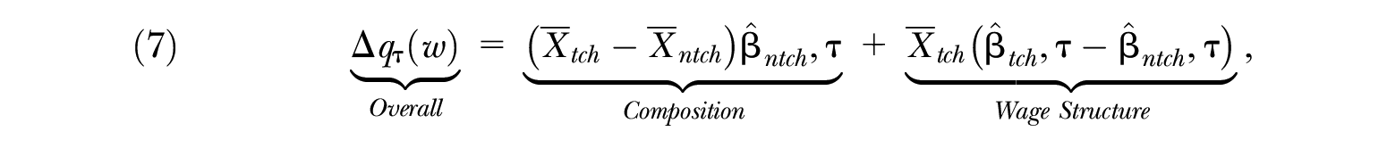
To account for this factor, I use the decomposition methodology advanced by Firpo, Fortin, and Lemieux (2007, 2009),
16
which decomposes wage differentials for quantiles in a similar manner to the standard Blinder-Oaxaca decomposition for the mean differential (Blinder 1973; Oaxaca 1973). Since the decomposition builds on the concept of the influence function (IF), first I formalize the IF for quantile

In this setting, the IF is an indicator that equals

The conditional expectation of the RIF can be expressed as a linear function of the explanatory variables, which permits me to use the RIF-regression model in a framework of the OLS regression. Formally, the earnings function of the RIF takes the following form:

where
where
Figure 2 provides the basic insights into this approach, following Fortin, Lemieux, and Firpo (2011). Distribution
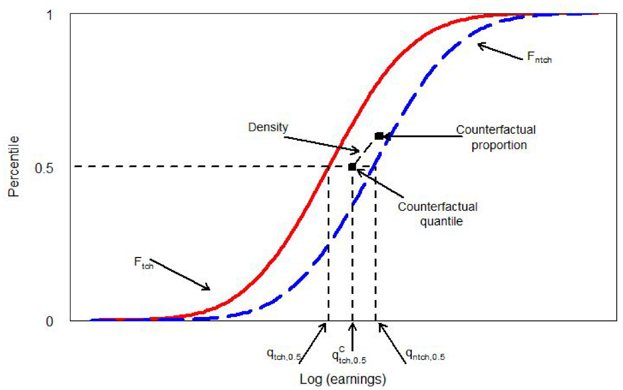
Illustration of Quantile Decompostion Approach
Before presenting the results related to the decomposition, I present the earnings gap across percentiles in Figure A.1 for female teachers and in Figure A.2 for male teachers, employing unconditional quantile regressions. The quantile coefficients on teachers can be interpreted as the effect of a change in the distribution of teachers, that is, a proportional increase in the share of teachers, on the earnings distribution. This exercise can be helpful in shedding light on teacher pay since the provision of teachers’ rigid salary schedules affects both the earnings gap between teachers and non-teachers at the mean and the distribution of earnings within teachers by not allowing an appropriate pay difference between high-skilled and low-skilled teachers. Estimates reveal noteworthy patterns in that the gap is positive at the bottom section of the distribution but becomes substantially negative at the upper section.
Next, I present the results for the decomposition based on Equation (7). The results exhibit the patterns of pay gaps and the returns to (individual and group) characteristics at various points of the distribution. As presented in Figure 3, estimates indicate that the overall difference between female teachers and non-teachers is substantially positive up to the 40th percentile. 18 I find the result at the 10th percentile to be especially striking, with the earnings differential between teachers and non-teachers being approximately 0.39 log points (approximately 47.7%). 19 Notably, the unexplained component is approximately 0.97 log points. Therefore, the wage schedule in the teaching sector favors teachers at the 10th percentile markedly, thus enabling them to enjoy a large wage premium. Overall, the wage structure effect illustrates that the earnings of female teachers up to the 60th percentile were not justified by their observed characteristics. In other words, they are paid a higher price for their skills than are non-teachers. Conversely, at the 90th percentile, the pay difference between female teachers and non-teachers is –0.41 log points (–50.67%). Of this difference, 0.15 log points is unexplained. This finding suggests that those who are in higher percentiles of the distributions face a wage penalty for being teachers.
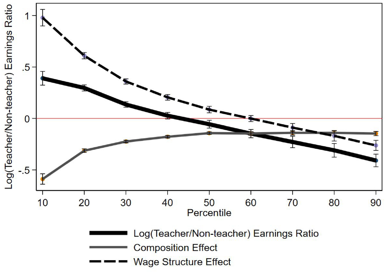
Quantile Decomposition of the Pay Gap: Women
For male teachers (Figure 4), the wage premium seems to be concentrated up to the 20th percentile. At the 10th percentile, the earnings gap between male teachers and non-teachers is 0.22 log points (24%). The unexplained gap is 0.44 log points, exhibiting a substantial wage premium. The overall wage premium for male teachers is not as high as that for female teachers. It disappears after the 20th percentile. Furthermore, the gap is negative and profound at the 90th percentile. The total difference at the 90th percentile for male teachers is –0.72 log points, and their characteristics, both individual and group, do not explain approximately 0.54 log points. This finding could be viewed as a wage premium for working in the non-teaching sector (and consequently a wage penalty for working in the teaching sector).
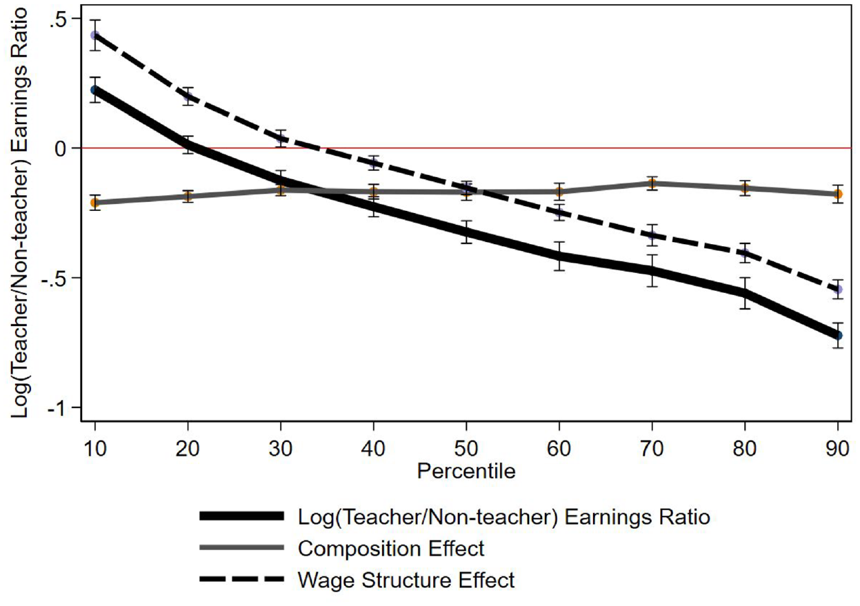
Quantile Decomposition of the Pay Gap: Men
These findings underpin how teaching is monetarily rewarding for some but provides a wage penalty for others. The differential effects at various percentiles explain why it is difficult to attract teachers from the top quantile of the ability distribution (Corcoran, Evans, and Schwab 2004; Hoxby and Leigh 2004; Bacolod 2007).
Discussion and Conclusion
In this article, I document new and robust findings concerning the earnings gap between teachers and non-teachers, using various techniques not previously considered in the literature. I provide evidence that a standard regression model that controls only for basic characteristics such as race, age, and education severely biases pay gap estimates between teachers and non-teachers. After addressing various biases, I show that female teachers earn 5 to 10% more than similar female non-teachers earn. My estimates of the earnings penalty between male teachers and male non-teachers are up to two-thirds lower than estimates obtained using a standard regression model as presented in the previous literature.
In interpreting the results, one caveat is especially noteworthy. This study does not consider other important aspects of compensation, including fringe benefits such as health insurance, retirement benefits, and job security. Unlike regular salaries, it is challenging to quantify how generous fringe benefits in the teaching sector are relative to the non-teaching sector because of the paucity of data in household surveys. Nevertheless, it is important to consider a few specific fringe benefits.
First, job security is a notable feature of the teaching profession. With job instability becoming more common in the modern labor market (Farber 2010) and job loss producing several monetary and psychological costs, individuals should place importance on having a secure job such as teaching. Richwine and Biggs (2011) provided suggestive evidence that job security in teaching can carry a compensation of up to 8%. Second, retirement health insurance is another significant perk of being a teacher (see Podgursky 2011). Upon retirement, teachers can continue to utilize the health insurance coverage provided during their employment. This benefit is important considering that individuals who retire before reaching 65 years of age—that is, when they become eligible for Medicare—must pay a substantial premium for medical coverage. However, employer-provided medical benefits upon retirement are not widespread; instead, they are declining among private-sector professionals. Third, pension constitutes an attractive benefit to teachers. Koedel and Podgursky (2016) noted that approximately 90% of teachers are enrolled in defined benefit (DB) pension plans. Teachers receive an annuity based on their salary and years of service. Private-sector employees, however, are typically enrolled in defined contribution (DC) plans. Under the DC plan, employers make an annual contribution to a worker’s retirement fund as long as the worker is employed and the worker does not receive any pension.
This study’s findings, along with those of the previous studies, invite the question of why the pay gap between teachers and non-teachers persists. Under the standard theory of competitive labor markets, it is expected that in equilibrium, both the demand for and supply of labor determine wages, with the “law of one price” holding a central role. Such conditions would lead teachers and non-teachers with similar skills to earn similar wages, thereby erasing the pay gap. Frictions in both teaching and non-teaching sectors, however, such as a licensure requirement, transferability of skills across sectors, tenure for teachers, and school administrators’ preferences for and ability to identify highly competent teachers, hinder movement between the sectors. Thus, the labor market is seemingly unable to clear the earnings gap.
This study yields several implications for designing K–12 education policies. Framing the findings using Roy’s (1951) model of occupational choice provides helpful insights into how school districts could improve their policies. Using a comparable comparison group turns an earnings penalty between female teachers and non-teachers into an earnings premium and erases most of the earnings gap between male teachers and non-teachers, indicating the possibility of their skill-based sorting. The wage rigidity in the teaching sector should have made it an attractive occupation for individuals with relatively lower skills. Conversely, highly skilled individuals may have self-selected into occupations that yield higher prices for their skills. Relatedly, one explanation for a rising gap in unadjusted earnings between teachers and non-teachers in recent decades, as documented in the literature, could be that the rising prices of skills in the non-teaching sector and skill-based sorting have led to higher earnings in the non-teaching sector. When such sorting occurs, a standard regression that controls for basic demographic information such as education and race biases pay gap estimates.
These findings also highlight the implication that policymakers should carefully assess the differential ability distribution of teachers and non-teachers to devise an optimum teachers’ salary schedule. Instead of merely considering the salary of non-teachers, school districts should focus on how various teachers’ skills are priced in the non-teaching sector. The decomposition of earnings across the entire distribution offers additional corroborating evidence on the potential selection of individuals into teaching based on their ability. The prevailing, rigid pay schedules that do not support differential pay structures based on qualification and competence are the main reason some teachers enjoy a wage premium while others face a wage penalty. Therefore, school districts should adopt a teacher’s compensation mechanism that provides differential and appropriate returns to skills. Specifically, they may want to differentiate the salary schedule according to the teacher type (e.g., primary or secondary) and by their subject of teaching. Doing that can help school districts attract and retain qualified individuals and avoid overpaying some teachers, leading to efficiency gains in their resource allocations.
Supplemental Material
sj-pdf-1-ilr-10.1177_00197939211072538 – Supplemental material for New Evidence on Teacher Pay
Supplemental material, sj-pdf-1-ilr-10.1177_00197939211072538 for New Evidence on Teacher Pay by Krishna Regmi in ILR Review
Footnotes
References
Supplementary Material
Please find the following supplemental material available below.
For Open Access articles published under a Creative Commons License, all supplemental material carries the same license as the article it is associated with.
For non-Open Access articles published, all supplemental material carries a non-exclusive license, and permission requests for re-use of supplemental material or any part of supplemental material shall be sent directly to the copyright owner as specified in the copyright notice associated with the article.