
Abstract
Overbraiding allows the production of complex hollow composite preforms. Various mechanical modelling methods have been proposed in the literature to help optimizing this process. However, these are either analytical, and computationally fast, but limited to axisymmetric braiding, or based on finite element methods (FEM) but computationally very expensive. The present work proposes a novel approach to model mechanically and in a computationally efficient manner the braid along its formation and deposition. Thereby, the geometrical and mechanical equilibrium of the whole braid in the convergence zone is described without symmetry assumption using a system of equations which is solved using the Newton-Raphson method. The new model, treating yarn-yarn friction, is evaluated using results from the literature, and demonstrates that friction is not the only physical mechanism that must be considered to simulate accurately the process. Finally, significant calculation time reduction is obtained compared to the most recent FEM simulations.
Introduction
Process overview
Overbraiding is a textile process that enables the production of complex hollow preforms for composite manufacturing. It presents the advantages of being almost continuous and highly automatable. The biaxial braiding machines are circular and equipped with two groups of spools located on its periphery. The two groups of spools circulate in opposite directions moved by carriers in a sinusoidal pattern. This movement causes the yarns to interlace and thus forms the braid. Each spool is coupled with a tensioning system that imposes a desired tension in the yarn. The other end of the yarn is fixed on a mandrel which has the shape of the desired composite part and which is driven through the center of the machine. The region of the braid located between the spools and the mandrel is called the “convergence zone” and the point of contact between the braid and the mandrel is called the “fell point”. Figure 1 presents the typical aspect of a braiding machine. During braiding, each yarn is subjected, to various mechanical loads generated by the tensioning system of the spool, the interactions with the other yarns and with the potential guiding ring. In order to obtain the desired mechanical properties for the final composite part, the deposition of the yarns with the desired braid angle and mandrel covering factor is of particular importance. Nowadays, the process optimization (mandrel trajectory and velocity, spool rotation speed) to reach the optimal process window is mostly realized experimentally. It requires a significant number of trial and error tests consuming material and time. In this context, simulation appears to be an interesting solution to help optimize the process.
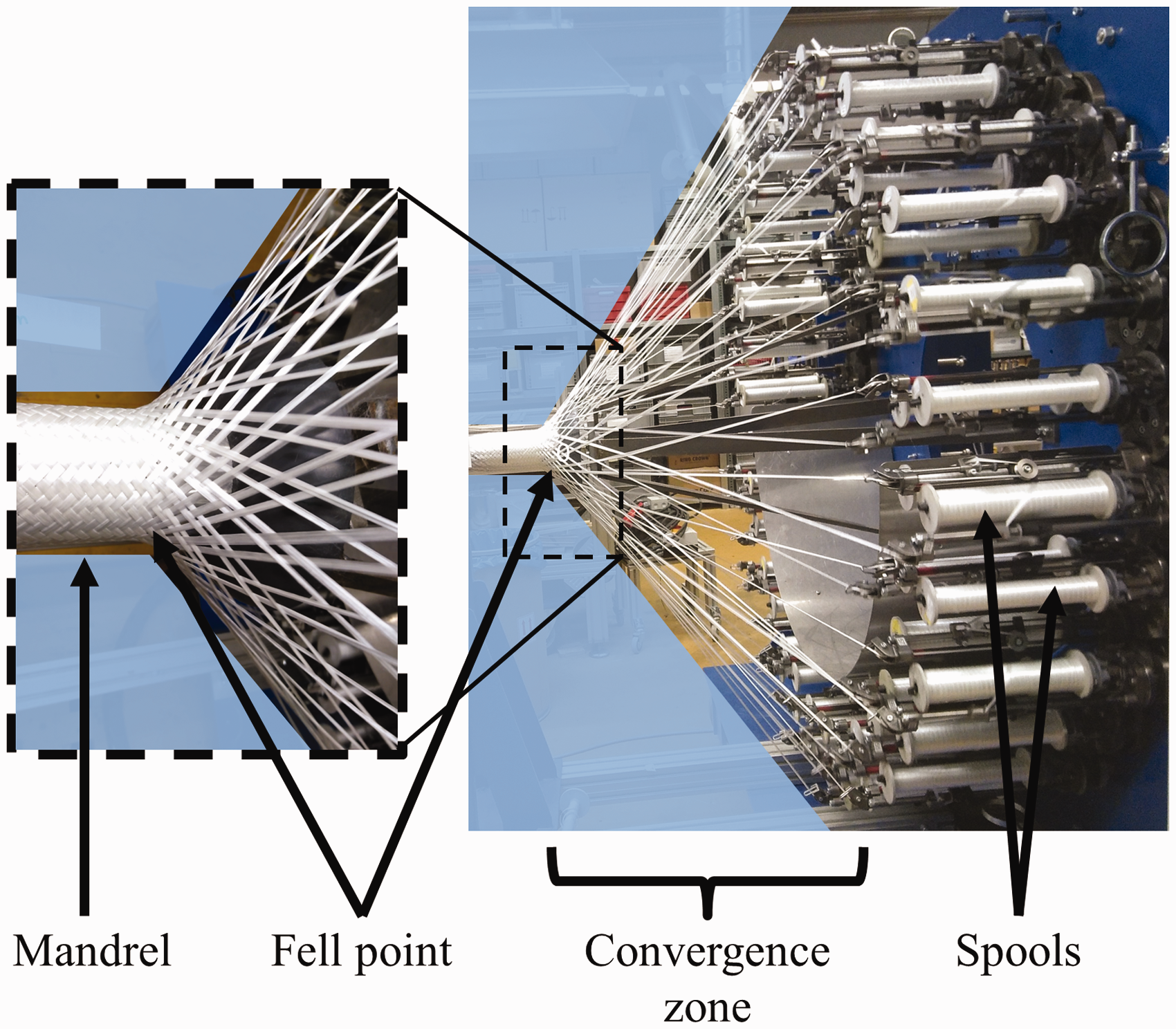
Lateral view of a braiding machine during braiding.
Previous works
Braiding simulations aim to predict accurately the characteristics of the future manufactured braid and simultaneously at determining the process parameters ensuring the specified braid properties. The mostly investigated modelling method for the braiding process is the direct solution. It consists in reproducing analytically or numerically the experimental braiding. The kinematics of the spools and of the mandrel are inputs, various yarn-yarn interaction models can be used to determine the yarn path in the convergence zone, and the braid characteristics are outputs of the simulation. On the other hand, the inverse solution consists is using a desired braid angle as input and predicts the required mandrel and spool positions which enable to obtain this deposition braid angle. The approaches used to obtain the direct or inverse solution to braiding modelling can be classified in three categories. A first approach is the kinematic modelling. The representation of the braiding model during kinematic modelling is fully geometrical and does not consider any force or energy. Du and Popper proposed an axisymmetric kinematic model in Du Popper. 1 Kessels and Akkermann extended the method to non-axisymmetric configurations in Kessels and Akkerman. 2 Inverse solutions to braiding modelling based on a kinematic model have also been proposed.3,4 The advantage of the kinematic approach is the short calculation time: in Kessels and Akkerman, 2 the calculation time is reported to be in the order of minutes for complex mandrel geometries. However, the accuracy of the obtained results is limited by the neglected yarn-yarn interactions. A second approach is the mechanically enhanced kinematic modelling in which some mechanical interaction equations are enhancing the geometrical kinematic modelling. Two major works have been published using this approach: Zhang et al. proposed in Zhang et al.5,6 a method assuming a conical convergence zone and van Ravenhorst and Akkermann proposed a method considering a non-developable convergence zone. 7 In these two methods, frictional effects are implemented which increases the accuracy of the process modelling compared to the kinematic models. However, the models stay limited to axisymmetric braiding configurations. Regarding the computation method, due to the set of equations that must be solved, the method used in literature5–7 are respectively the Newton-Raphson method and a non-linear optimization method and can be thus classified as numerical. A third approach is the mechanical modelling which is based on the use of finite element interacting with each other after applying the proper boundary conditions. These methods allow treating various interaction mechanisms (frictional yarn-yarn or yarn-mandrel contact), as well as the undulation and bending behavior of the yarns. Finite element mechanical modelling of the braiding process has been shown to generate satisfying braid angles on complex mandrel shapes.8–11 However, an industrial use of such techniques remains difficult due to the very long calculation times, in the range of several hours to days depending on the number of yarns and the length of the mandrel.10,11 For these reasons, the FE method does not appear as a promising solution to allow a fast process optimization. In this context, the mechanically enhanced kinematic approach could be an interesting method to allow a fast and accurate modelling of the braiding process if it could be extended to non-axisymmetric braiding conditions.
It must be finally emphasized that whilst not addressing the mechanics of the yarns in the braiding process in particular, the problematics of elongated and flexible bodies subjected to various loadings has been intensively investigated and theorized in the frame of structural mechanics in publications dedicated to cables.12,13 In these publications as in Zhang et al., 6 the equilibrium of the cables (or of the yarns) is presented in the form of a set of equations, and a numerical method is proposed to determine the geometrical and mechanical unknowns by solving the set of equations. As the braid in the convergence zone is a group of yarns (i.e. cables) interacting with each other at their contact points, it appears that solving a system of equations describing the global equilibrium of the braid is a promising method to model the braiding process.
Objectives
A new mechanically enhanced kinematic modelling method allowing the fast simulation of braiding over non-axisymmetric mandrels could be of great interest for industrial process optimization. Additionally, the principle of solving a system of equations describing the whole braid equilibrium in the convergence zone appears promising because of its ability to take into account every interaction simultaneously to predict of the braid characteristics. The goal of the presented work is therefore to introduce a mechanically enhanced kinematic method, based on this principle. This method would feature the advantages of being computationally fast through the use of a numerical calculation technique and allow the analytical mechanical modelling of the braiding process for non-axisymmetric configurations, including friction and deposition. It would therefore exhibit novelties compared to the axisymmetric analytical interaction model presented by van Ravenhorst and Akkerman 7 as well as calculation time reduction compared to the recent FEM simulations. 11 In the frame of this work, the implemented physical phenomena are yarn undulation and frictional yarn-yarn interactions. Nevertheless, the presented model could serve as basis for the implementation of further physics, as evolution of the yarns cross sections or yarn-yarn lateral interactions in jamming conditions.
Proposed model
General principle
The present method consists in generating and solving a system of equations that describes the global geometrical and mechanical equilibrium of the braid in the convergence zone. The characteristics of the braid being built (yarn angles, lengths between the interlacing points, yarn-yarn interaction forces, etc.) are unknown and are obtained by solving the system of equations for the successive spools and mandrel positions. The boundary conditions (spool and mandrel position) are updated according to the given process parameters. The position of the fell point of each yarn is updated whenever a segment has been deposed on the mandrel. The final braid characteristics are determined through the successive deposition of braid segments on the mandrel. The resolution of the system of equations for arbitrary boundary conditions and interaction configurations ensures the ability of the model to treat any of the configurations met during the overbraiding of complex industrial parts.
Assumptions
The braiding process is assumed to occur in a quasi-static manner so that the braid can be considered in the convergence zone at any time in geometrical and mechanical equilibrium. The yarns are considered inextensible as the tension applied commonly on the yarns during the braiding process is below 10 N6,7 which is not expected to generate significant axial deformations for glass or carbon yarns. Additionally, the bending stiffness of the yarns is neglected. Mass and therefore inertial effects are also neglected. No assumption is made on the shape of the cross section of the yarns. The shape of the yarns is simply defined by a constant thickness which is the half distance between two yarns at their interaction point. The yarns feature no reaction force to lateral compaction. Yarns are defined by their centerline, which is composed of straight segments between the interlacing points and are assumed to be fixed to the mandrel at the fell point. For each successive step, the position of the ends of each yarn on the mandrel and on the spool are known. The value of the yarn tension in the segment directly before the spool (or before the ring, depending on the considered configuration) is imposed by the tensioning system of the spool. The number of interlacing points on each yarn as well as the sequence of the intersected yarns is also considered as known. Accordingly, the choice has been made to model the braiding process in geometrical configurations in which yarn-yarn contacts are surely occurring. Two equivalent configurations are considered:
The braiding machine is modelled without ring. The spools are assumed to move on the spool plane. The braiding machine is modelled with a ring and only the region between the ring and the fell point is modelled. Each yarn is assumed to be in contact with every crossed yarns between the fell point and the ring.
Finally, yarn-yarn friction is considered in the model as forces localized at the interaction points.
Loadings on the yarn
Four types of loadings are assumed to be applied on the yarns:
Boundary forces
As the yarns are assumed to be fixed on the mandrel at the fell point and on the machine at the spool (or on the ring depending in the configuration), these two fixation points apply the boundary forces to the yarn.
Tension from the spool tensioning system
The tension is a force which is aligned with each segment of the yarn. The segment of each yarn preceding the spool is subjected to the known tension of the spool tensioning system. In the other segments, the value of the tension is unknown.
Yarn-yarn normal interaction forces
The yarns are subjected to interaction forces from the other yarns at the interaction points. One component of this interaction force is a normal force which is characterized by its normality to both yarns. Additionally, it is aligned with the line connecting the center of each yarn at the interaction point.
Yarn-yarn friction forces
At each yarn-yarn interaction point is acting a friction force. This friction force is directed in the opposite direction of the relative motion of the contacting points. Furthermore, it is assumed that the friction force depends on the norm of the normal force. 14 The calculation of the friction forces is described in Appendix 1.
Identification and numbering of the unknowns
Geometrical unknowns
As introduced in ‘Assumptions’ section, each yarn
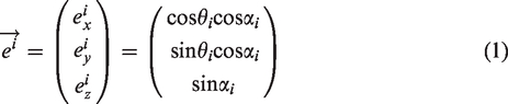
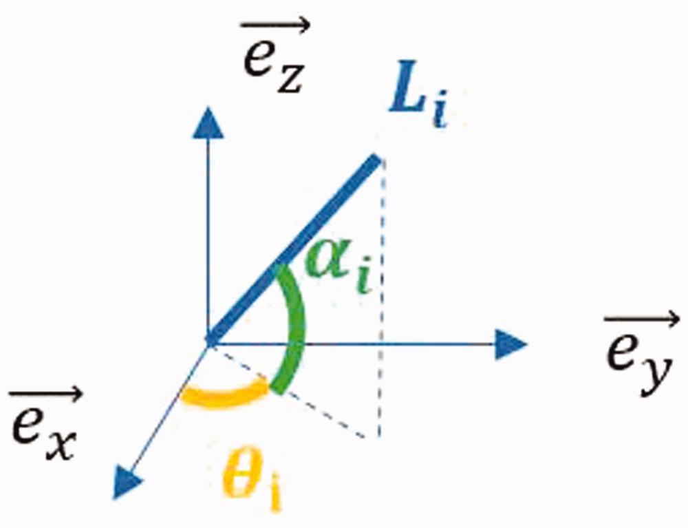
Geometrical definition of the segment Si.
Therefore, for each yarn
Mechanical unknowns
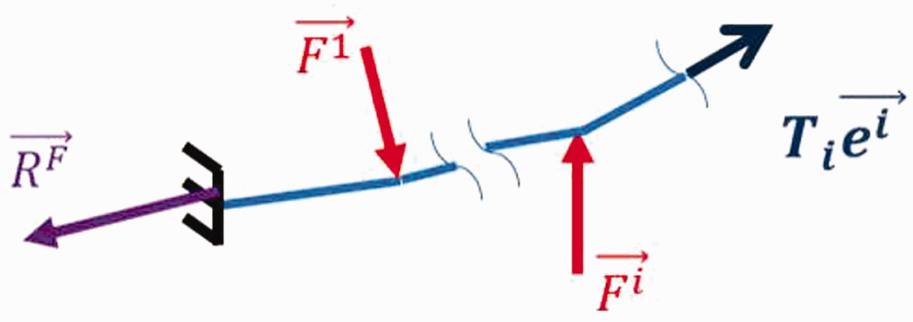
In order to physically determine the braid equilibrium, mechanical quantities need to be determined. Figure 3 shows a generic view of a yarn with the applied loads. These quantities are:
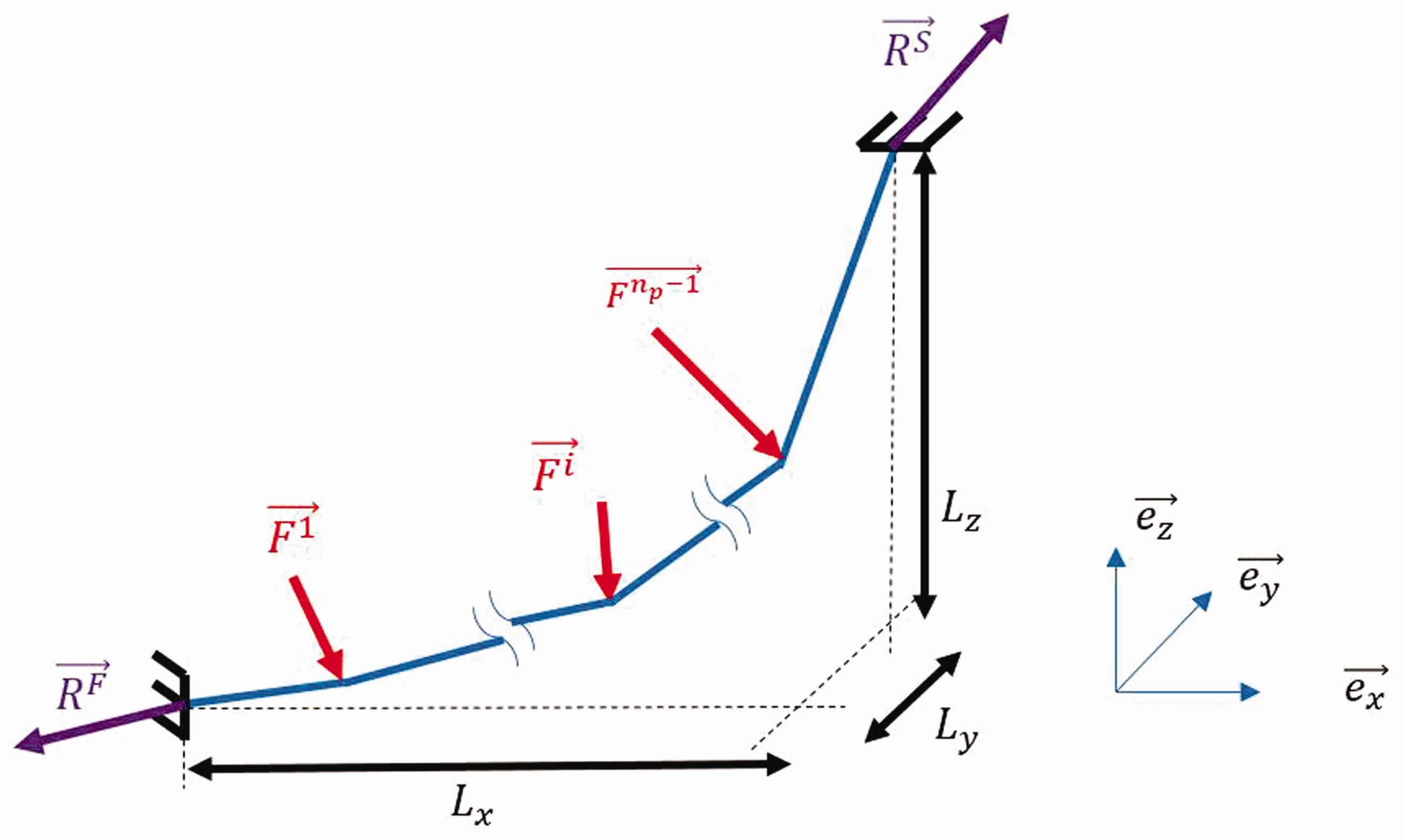
Schematic view of the external loads applied on a yarn.
Three force components at the fixed end of the yarn on the fell point
Three components of normal interaction force
One value of tension
Total number of unknowns
Table 1 summarizes, the theoretical number of geometrical and mechanical unknowns required for each yarn
Theoretical number of unknowns required to characterize completely the braid equilibrium.
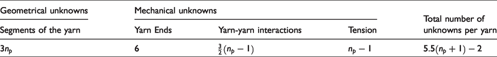
Therefore, the total theoretical minimal number of unknowns for a complete braid made of
Equations describing the braid equilibrium
In order to determine the unknowns, the same number of equations must be written and the obtained system must be solved. The equations describing the equilibrium of one yarn, and of the yarn-yarn interaction points, are detailed in the following subsections. The equilibrium of each yarn and of the interaction points ensures the equilibrium of the whole braid.
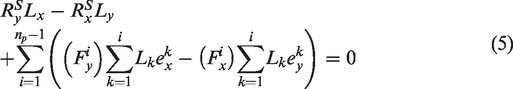
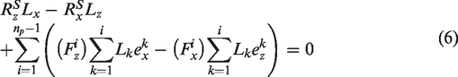
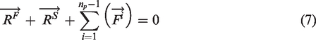
Yarn global equilibrium
Six equations are used to describe the global geometrical and mechanical equilibrium of a yarn. Equation (4) defines and imposes the distance 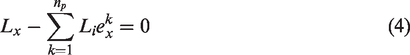
Local tension equilibrium
At equilibrium, each segment 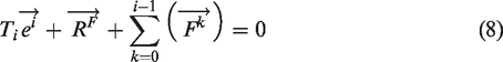
Representation of the local force equilibrium of the segment i.
It must be noticed that for equation (8), if
Equilibrium of a yarn-yarn interaction point
From a geometrical point of view, when two yarns featuring a negligible thickness intersect, the points of interaction on both yarns have the same spatial coordinates. In practice, however, the yarns have a non-zero thickness. This means that the two interaction points are separated by a distance 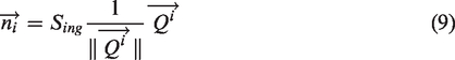
In equation (9), 
Equation (11) defines mathematically, the interaction of two yarns and a schematic view of a yarn-yarn interaction can be found in Figure 5.

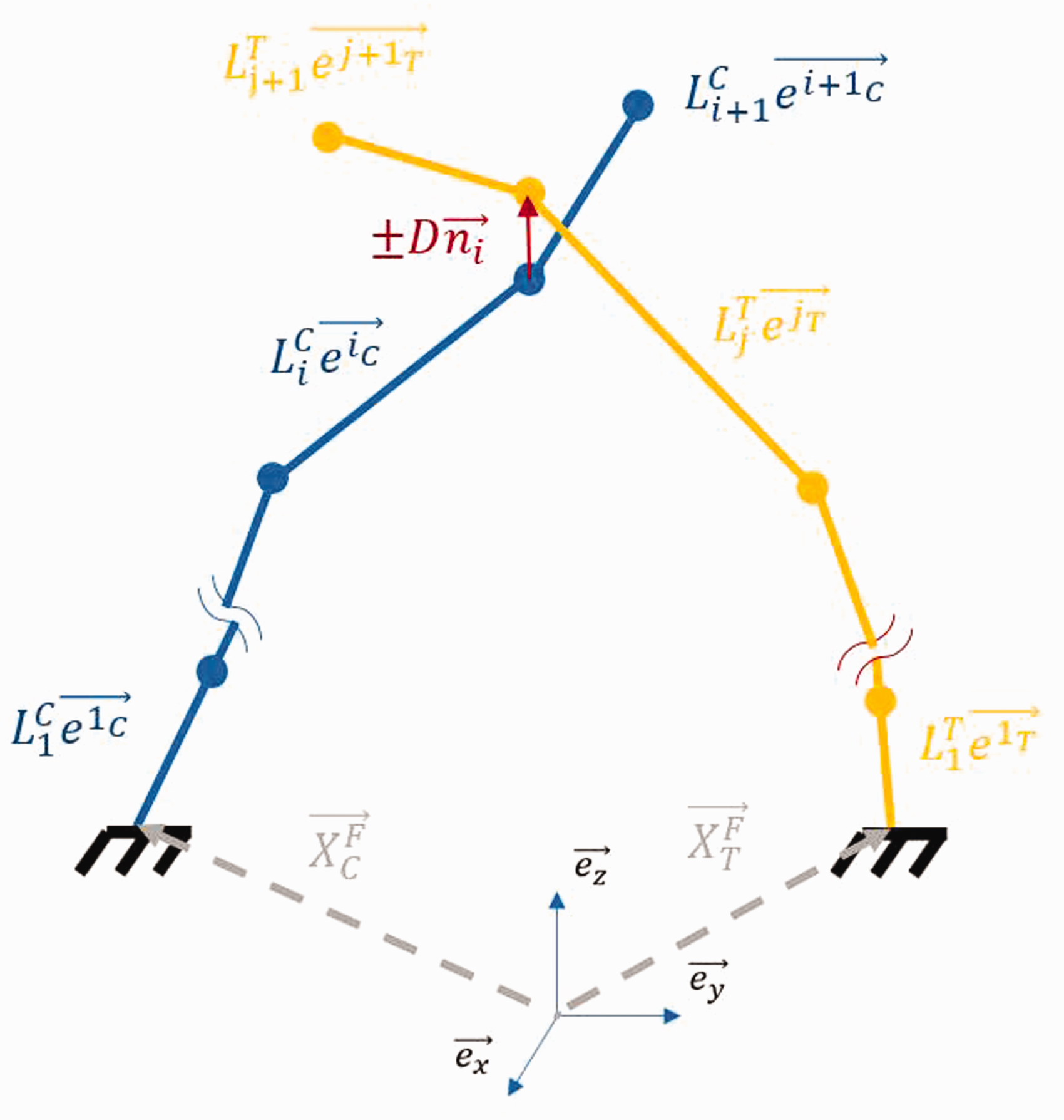
Geometrical definition of an interaction point.
In equation (11),
Normality of the yarn-yarn interaction force
As introduced in the previous section, the normal interaction force between two contacting yarns is perpendicular to these two yarns. This can be mathematically expressed as the fact that the scalar product of the interaction force with the local direction of the yarn at the yarn-yarn contact point must be equal to zero. The local direction of the yarns is defined as the sum of the vectors orienting the segments surrounding the interaction point. Interaction force normality is thus imposed in the model using equations (12) and (13). The validity of this definition will be demonstrated in ‘Braiding pattern’ section.


Total number of equations
The number of equations required to define a braid equilibrium is summarized in Table 2.
Number of equations required to describe the braid equilibrium.
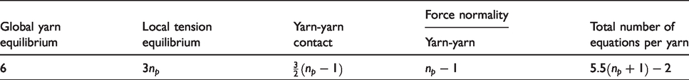
It can be seen in Table 2 that the total number of equations describing the braid equilibrium is equal to
Numerical method for braiding modelling
The system of equations presented in the previous section defines the geometrical and mechanical equilibrium of the braid. If a set of unknown can be found, that allows satisfying all the equations of the system, this set of values is the set of solutions of the system and defines the characteristics of the braid for the considered equilibrium. Several numerical methods are available in the literature 15 to solve non-linear systems of equations (Newton-Raphson, Broyden’s method, etc.). In the presented study, the choice has been made to use the Newton-Raphson method.
Newton Raphson method
The Newton-Raphson method determines a set of solutions for a considered system of equation in an iterative manner. Starting from an initial set of guesses 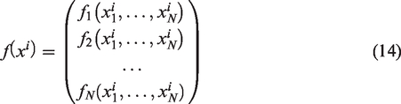
In equation (14) the 
In equation (15), 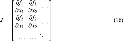
As highlighted in ‘Equations describing the braid equilibrium’ section, the equations describing the braid equilibrium are expressed analytically. For this reason, it is possible to calculate analytically the partial derivatives of the functions
Braiding algorithm
Initiation of the braiding simulation
The modelling of the braiding process begins with a defined position of the mandrel and of the spools and a defined yarn tension in each yarn. This initial configuration is chosen so that the yarns feature one yarn-yarn contact. A first guess of the unknowns is made assuming straight yarns, a constant tension in all segments of each yarn and normal forces featuring a small value (1/100 of the yarn axial tension) and being directed normally to the two yarns. The initial guess for the length of the segments on the yarn is a fraction of the total length and is adjusted depending on the mandrel geometry and the machine or ring radius. The Newton-Raphson method is run until convergence. The first state of equilibrium has been determined.
Further simulation steps
In order to ensure representative deposition braid angles from the beginning of the mandrel, the spools are rotated until first deposition is observed on the mandrel. Then, the proper braiding strategy (spool and mandrel velocities) is applied. Figure 6 presents the successive convergence zone configurations at the beginning of the exemplary overbraiding of a cylindrical mandrel. During steps 1 to 15, interaction points are added to the convergence zone by rotating the spools around the machine. At step 16, first deposition occurs. From step 17 on, mandrel begins to move relatively to the spool plane. This is done in practice by translating the spool plane.
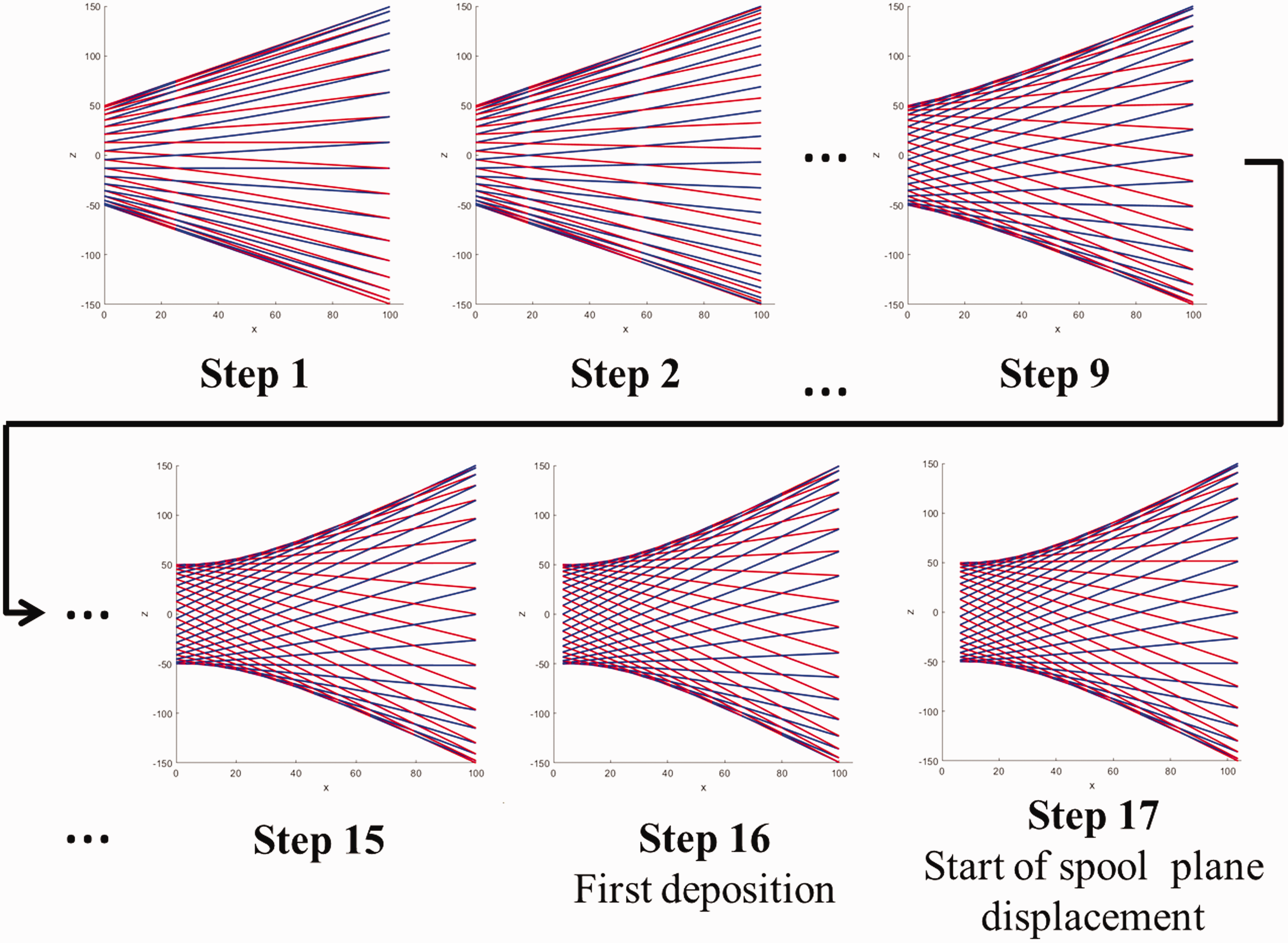
Convergence zone configurations at the beginning of the exemplary overbraiding simulation of a cylindrical mandrel.
In the braiding algorithm, the rotation of the spools is treated as follow. The spools are rotated either to run a fraction of the way to generate a new interlacement or to generate directly a new interlacement at each new equilibrium. If no new interlacement point is generated (if the clockwise and counter-clockwise spools have not crossed), the boundary conditions are updated and the solution of the previous equilibrium is used as first guess for the new equilibrium. When a new interlacement has been generated, the boundary conditions, as well as the sequence of yarns intersected between the fell point and the spools are updated. The values of the unknowns are kept from the previous state for all segments except the last segment of each yarn. This one is split into two segments featuring the same direction and the same tension. The initial guess for the normal force at the generated interlacement point is taken equal to the one at the last interlacement point in the previous equilibrium and its direction is adapted depending on the braiding pattern. On the other side of the convergence zone, the position of the fell point of each yarn is updated using the following strategy. It is evaluated for each interaction point, when each equilibrium is calculated, if the considered interaction point is located outside or inside of the volume defining the mandrel. If it is located outside, it is considered as not deposed. If it is located inside of the mandrel, it is considered as deposed. For each of the two interacting yarns, the unknowns of the deposed segment located between the previous fell point and the new fell point are removed from the list of unknowns and are saved. Finally, the fell point of the two interacting yarns is updated to be the newly deposed interaction point. Using this technique the position of the fell point of each yarn is thus a direct consequence of the braiding parameters. This technique enables therefore to reproduce the complexity of the fell point distribution morphology in non-axisymmetric braiding conditions without making assumption on the geometry of the fell point. For each new configuration, the Newton-Raphson method is used to calculate the new equilibrium.
Results and analyses
The claimed novelties of the presented work are its ability to model geometrically and mechanically the braid during its formation and deposition in non-axisymmetric braiding configurations with a reduced computational cost compared to FEM. Several validation tests have been conducted to verify these claims.
Capabilities of the model
The presented approach is based on the calculation of the mechanical braid equilibrium. As introduced in ‘Loadings on the yarn’ section, yarn-yarn interactions generate loadings on the yarns that must be considered in the model. In the following sections, the capability of the approach to treat yarn-yarn interactions is demonstrated as well as the capability to reduce computation time compared to FEM modelling.
Braiding pattern
Yarn undulation due to the interlacements of the yarns is implemented in the description of the braid equilibrium in equation (11). In Sun et al., 11 recent FEM simulation techniques have been used to simulate the braiding of 450 mm long cylinders with 36 yarns and a braid angle of 45°. Simulation parameters, listed in Table 3, are used in order to generate the same braid characteristics as in Sun et al. 11 with two different braiding patterns. The yarn thickness of 1.5 mm is large for the yarns used in the classical braiding process but it enables a better observation of yarn undulation due to yarn-yarn contact. One braid features a diamond (1/1) pattern (named Diamond for the rest of the document) and the second braid features a 2/2 regular braiding pattern (named Regular for the rest of the document). Figure 7 presents the view of the braid patterns obtained at the end of the simulation.
Process and simulation parameters for an equivalent braiding than the biaxial braiding of Sun et al. 11
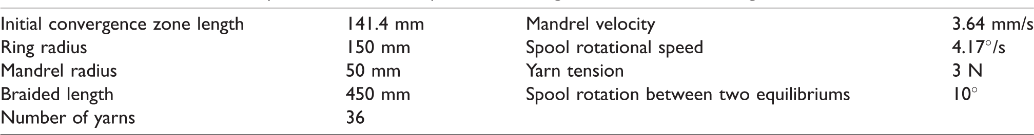
Aspect of the braiding pattern for Diamond and Regular braiding.
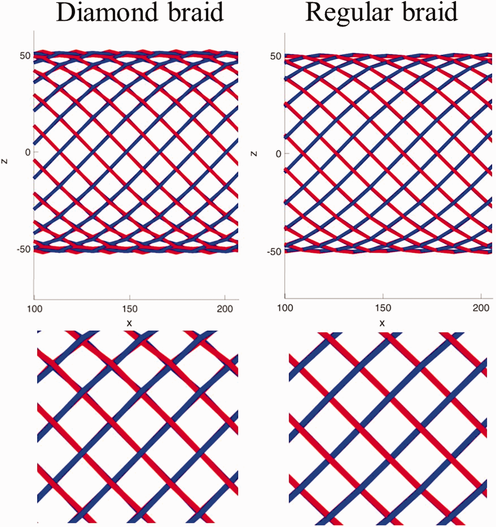
It can be seen in Figure 7 that the expected braiding patterns are successfully obtained: in the Diamond configuration, each yarn goes successively above one yarn and under one yarn and in the Regular configuration, each yarn goes above two yarns and then under two other yarns. Furthermore, the orientations of the normal interaction forces, which can be observed on Figure 8, reveal the appropriate alternation in both Diamond and Regular configurations ensuring that the influence of the braiding pattern on the yarn-yarn mechanical interaction is successfully taken into account. This demonstrates in a simple braiding configuration (cylindrical mandrel) that the desired braiding pattern can be imposed. Finally, in the considered frictionless conditions, no variation of the tension could be noticed in the various segments of the yarns. This demonstrates that the normality of the normal interaction forces to the yarns imposed in equations (12) and (13) is satisfied. Thus the normal interaction forces calculated by the model can be used for the calculation of the friction forces.
Normal interaction forces along one yarn for Diamond and Regular braiding.
Friction forces
As demonstrated in the previous section, normal yarn-yarn interactions satisfy the imposed conditions. Therefore the norm of the friction force, which is directly related to the normal force is considered as correct. Furthermore, as defined in Appendix 1, the direction of the friction force is given by the relative motion of the interaction points. It is obtained automatically by comparing on each yarn the position of the considered interaction point with the position of a point at the same yarn length in the reference configuration (a previous saved braid state). In order to verify that the developed technique provides the appropriate friction force direction, a validation test has been conducted in axisymmetric conditions. Figure 9 presents different views of the convergence zone at the moment of first deposition with friction force vectors at various interaction points. The braiding parameters are the ones of Table 3 with a doubled number of yarns (72 yarns in total), a yarn thickness equal to 0.3 mm and a Coulomb coefficient of friction of 0.3. The reference configuration to calculate the friction force is taken for every new step as the previous calculated step.
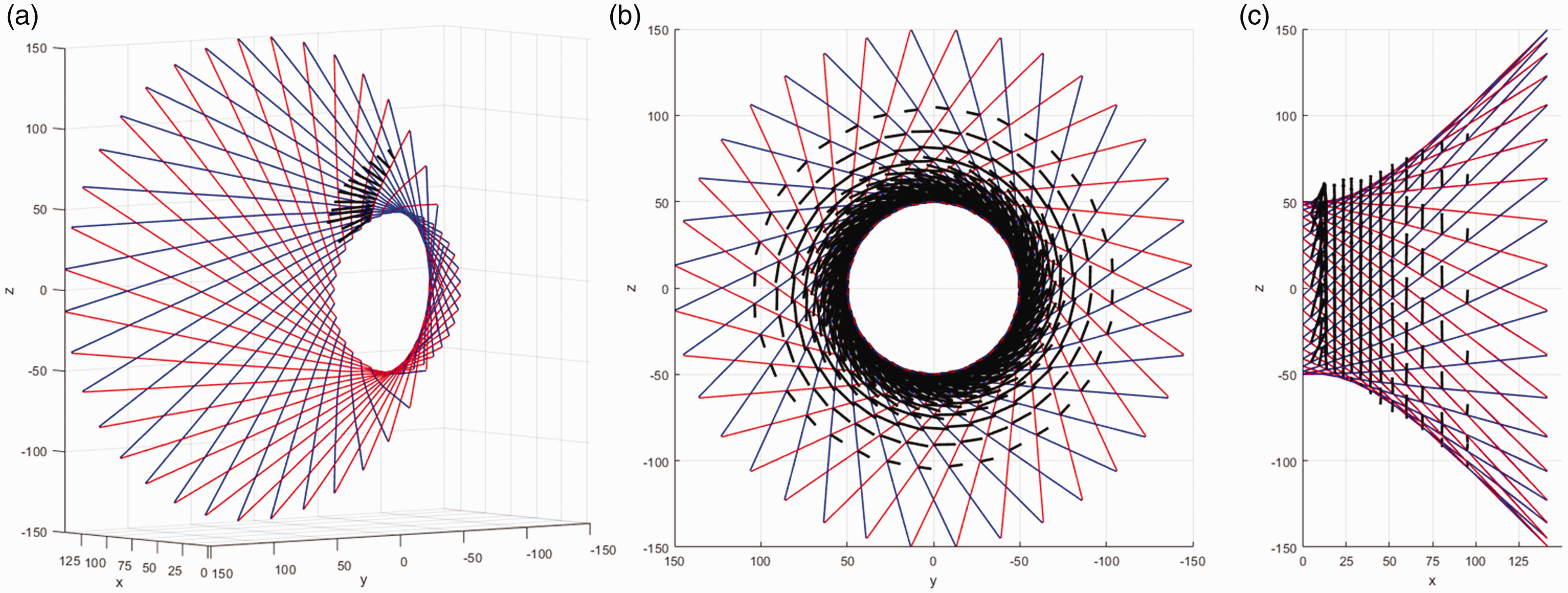
Various view of the convergence zone for a simulation with friction. (a) Perspective view. (b) Front view. (c) Side view. Friction forces are represented as black arrows. (x and z axes are expressed in mm).
Figure 9(a) displays a perspective view of the convergence zone and allows observing the curvature of the yarns induced, as expected, by friction. Figure 9(b) displays a front view of the convergence zone. The orientation of the friction forces along the “interlacement circles” (i.e. tangent to the braid and perpendicular to the braid axis) predicted by the analytical approaches of Zhang et al. 6 and Van Ravenhorst and Akkerman 7 can be well recognized. This orientation is confirmed by the side view of the convergence zone in Figure 9(c) for the interaction points away from the fell point. In fact, the orientations of the friction force vectors of the two first rows of interaction points are not following the “interlacement circles”. This is due to the combined facts that yarn thickness is taken into account in the calculation of the direction of the friction force and that just before deposition, the relative motion of the interaction points between two successive steps is very small. For this reason, the direction of the friction force is significantly affected by the undulation of the yarn within the braid. This can be demonstrated by the fact that this discrepancy in the friction force orientation to the alignment with the “interlacement circles” disappears when very small values of yarn thickness are used. This result could not have been predicted by the analytical models presented previously in the literature because only the “macroscopic” yarn motion generated by the rotation of the spools was considered. The presented model features therefore an improvement in the accuracy of the prediction of the friction forces compared to the previous analytical models. This result highlights also the fact that the model treats spontaneously non-axisymmetric friction forces configuration and that it is therefore appropriate for the simulation of non-axisymmetric braiding.
Additionally, a qualitative validation has been realized on order to ensure that the aspect of the convergence zone is in good agreement with reality. For this purpose, the braiding parameters of the simulation have been taken identical to the ones of a reference braiding experiment. These parameters are summarized in Table 4. The yarn paths in the convergence zone obtained from the simulation are compared with the yarn paths observed experimentally on the braiding machine in Figure 10.
Process and simulation parameters for the qualitative comparison of yarn paths observed experimentally and obtained from the simulation.
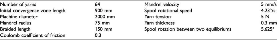
Comparison of the convergence zone observed experimentally and the convergence zone obtained by simulation using the developed model (blue and red yarns).
It can be observed in Figure 10 that a very good match is obtained between the simulation and the experiment. It can be first noticed that, in the convergence zone and on the mandrel, simulated and experimentally observed yarns are overlapping or very close in both braiding directions. The observed minor discrepancies are due to the experimental yarn clustering effect which is a consequence of the spool sinusoidal movement around the machine (this movement is not reproduced in the simulation). Thus, the very good agreement obtained between experiments and simulation confirms qualitatively and for the considered braiding conditions, the ability of the model to reproduce accurately the yarn path in the convergence zone. Quantitative investigations of the capabilities of the method to predict braid angle are presented in ‘‘Simulation of braid deposition and discussion’’ section.
Non-axisymmetric braiding conditions
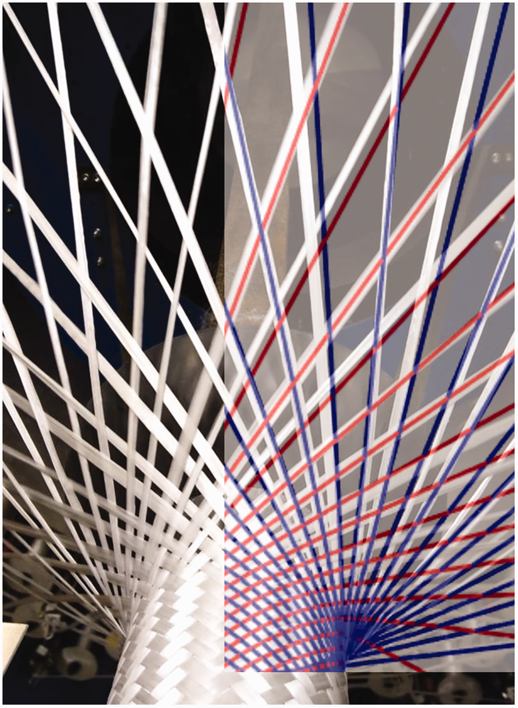
Qualitative tests have also been realized in order to evaluate the capability of the method to treat non-axisymmetric braiding conditions. Figure 11 represents two cases of successful simulations: the overbraiding of a cylindrical mandrel driven with a radial offset into the braiding machine in Figure 11(a) and the overbraiding of an elliptical mandrel featuring an eccentricity of 0.87 in Figure 11(b).
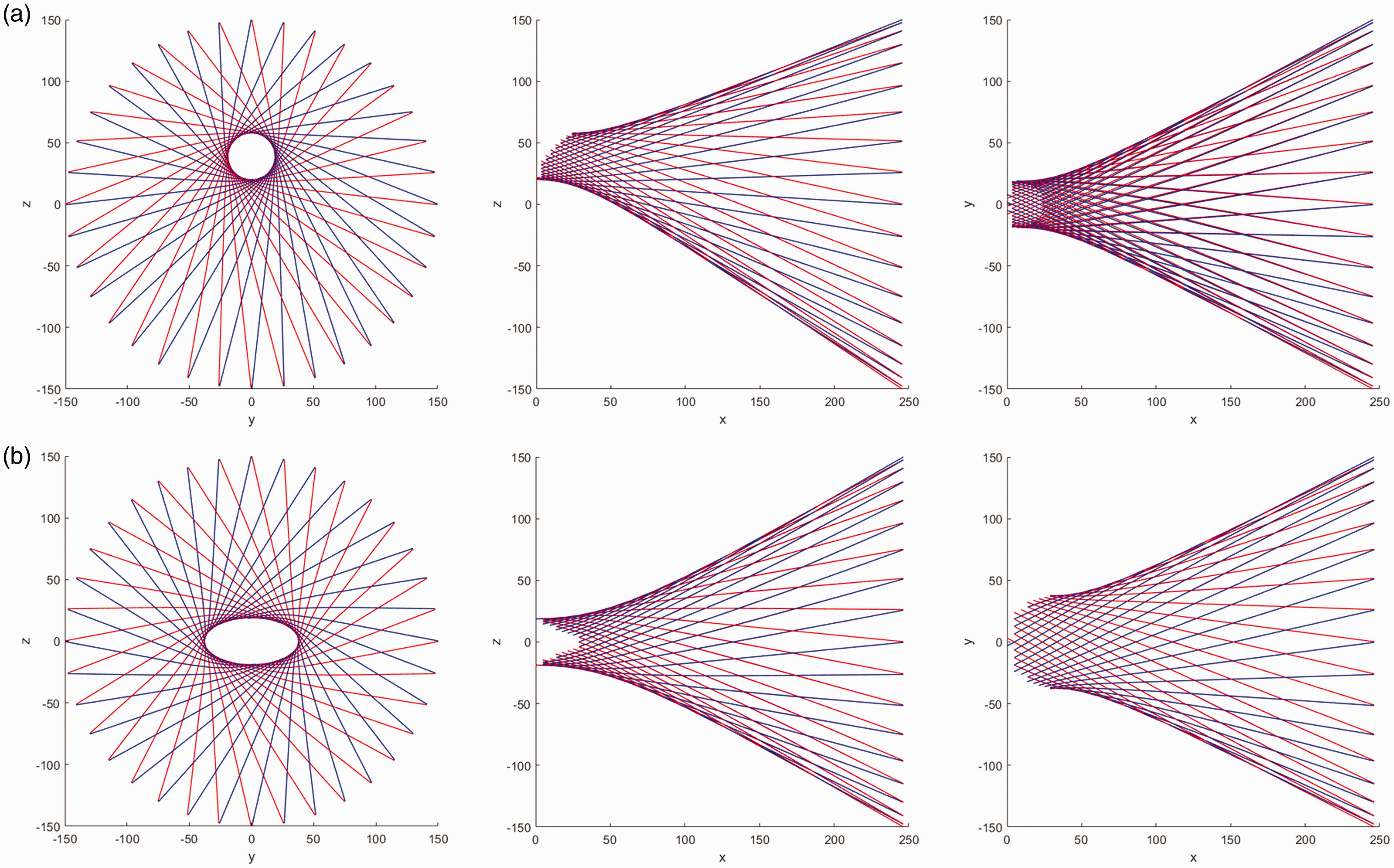
Aspect of the convergence zone for exemplary non-axisymmetric overbraiding. (a) Case of a cylindrical mandrel driven with a radial offset in the machine. (b) Case of an elliptical mandrel (x, y and z axes are expressed in mm).
In Figure 11, only the yarn segments which have not been deposed are represented. This enables to study the fell point distribution morphology. It can be observed in Figure 11(a) and Figure 11(b) that a complex fell point distribution morphology has been obtained. This highlights the capability of the method to treat the overbraiding of mandrels in non-axisymmetric conditions.
On the other hand, limitations are encountered for mandrels featuring sharp edges. Figure 12 represents a front view of an overbraiding simulation of a mandrel featuring a square cross section.
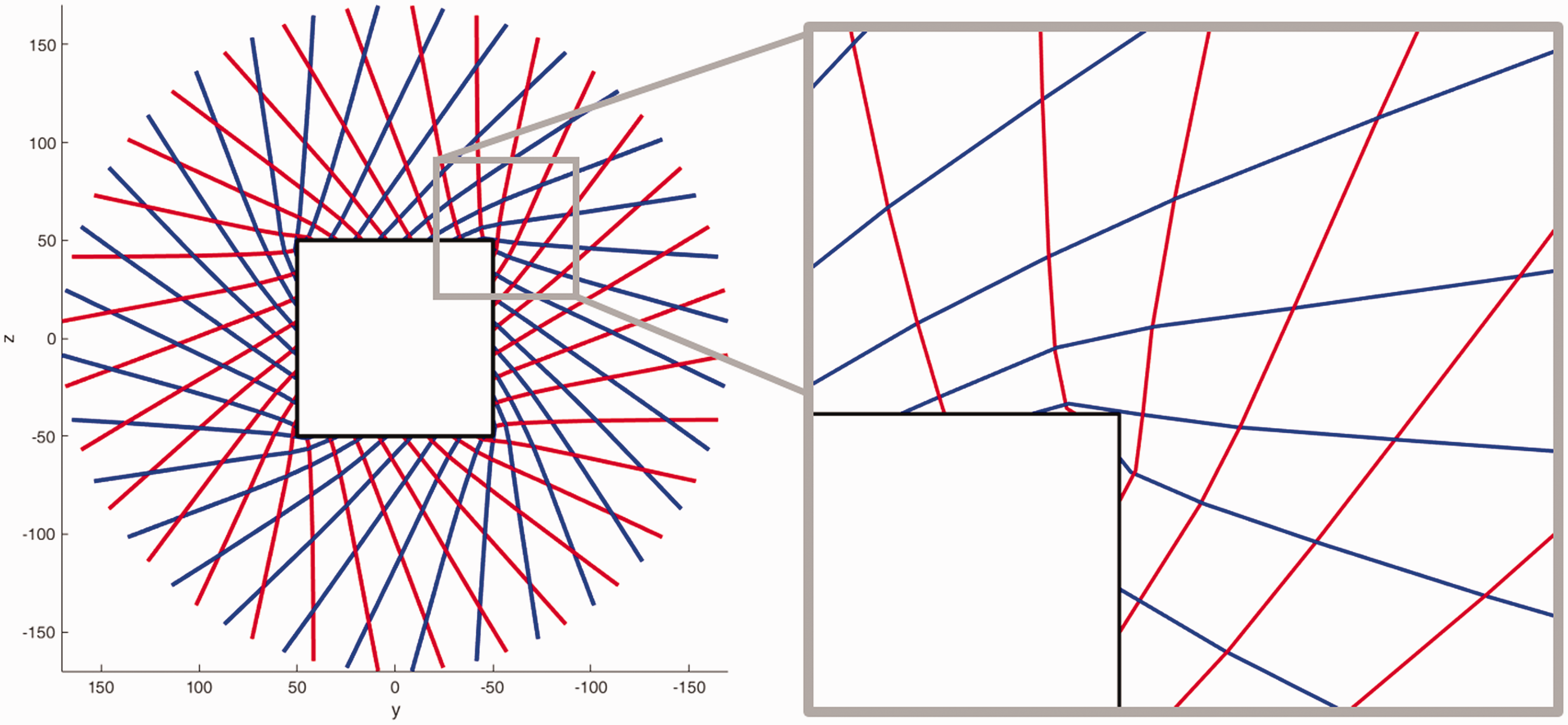
Front view of the overbraiding of a square mandrel with the presented method (y and z axes are expressed in mm).
It can be observed in the zoomed part of Figure 12 that the blue yarn is coming in contact with the edge of the mandrel before the interaction point between this contact point and the fell point has deposed on the mandrel. The movement of the yarn-mandrel interaction point should be therefore imposed to follow the edge until the yarn-yarn interaction point has deposed. This would require the implementation of yarn-mandrel interactions into the model which has not been realized in the so far developed model.
The presented model enables therefore to treat more complex braiding configurations than the mechanically enhanced kinematic models presented in the literature.5–7 This ability will be used to validate quantitatively the novelties of the presented method on experimental results from the literature in ‘Simulation of braid deposition and discussion’ section. Further developments on yarn-mandrel interactions will be required in order to extend the treatable mandrel geometries to mandrels with sharp edges.
Calculation time
Comparisons in terms of calculation time can be realized with the calculations made in Sun et al. 11 In Sun et al., 11 the average calculation is reported to be running on 16 cores for one hour. The braiding simulation of an equivalent braid (same number of yarns, same braid length, same deposition angle) lasted 78 s without friction and 97 s with friction using 8 cores with the developed analytical method implemented in Matlab. Therefore, for the considered configuration, the simulation finishes faster than the modeled experimental process (124 s of real braiding time). This represents also a reduction of the calculation time of more than a factor 37 compared to Sun et al. 11 and demonstrates therefore the potential for reducing the calculation time with the proposed method compared to FEM.
Simulation of braid deposition and discussion
In the previous section, the ability of the method to treat accurately frictional yarn-yarn interactions and non-asymmetric braiding conditions in a computationally efficient manner has been demonstrated. In the current section, the ability of the method to predict deposition angles will be investigated. Comparisons are made with experimental results from the literature.
Braid deposition in axisymmetric conditions
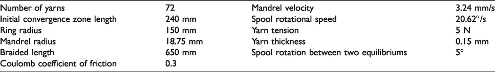
Validations of the model are realized first in axisymmetric conditions using the experimental data of one of the experiments of Du and Popper. 1 In the considered experiment, a biaxial braiding machine with 72 carriers is used to realize a 2/2 Regular braid. The yarns are assumed to be in contact with the ring. The braiding parameters are summarized in Table 5. Simulations are realized without friction and with a Coulomb coefficient of friction of 0.3, which is in agreement with experimental values reported in the literature.7,9 After the first deposition, the spool plane starts moving with the prescribed mandrel velocity. In the simulation, the spool rotation between two successive equilibriums is 5° which corresponds to the generation of a new interlacing point at every new equilibrium. Figure 13 presents the results of the simulation after 0.848 s, 32.9 s, 69.3 s, 106 s and 142 s of frictionless braiding.
Process and simulation parameters for the modelling of the experiment of Du and Popper 1 .
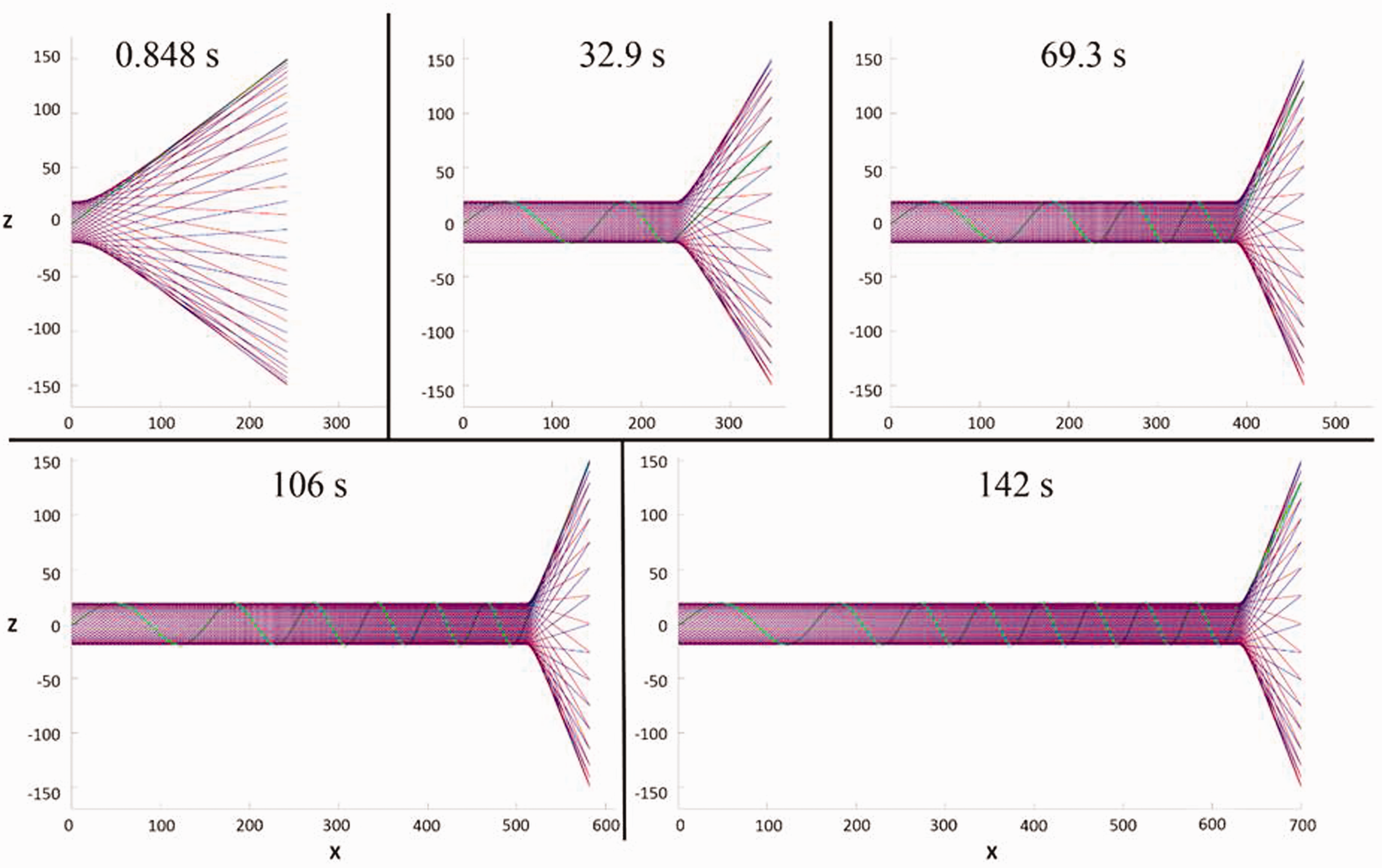
Aspect of the braid at different moments during frictionless overbraiding of a cylindrical mandrel (x and z axes are expressed in mm).
Two major observations can be made in Figure 13: first, the length of the convergence zone reduces along braiding to reach a constant length. This phenomenon has been observed experimentally by Du and Popper.
1
It is due to the fact that the initial convergence zone length has been chosen longer than the convergence zone length expected in stationary conditions. The second observation is that the braiding angle increases significantly along the length of the mandrel. In the present case of axisymmetric braiding, the braid angle along one yarn is representative of the braid angle of all the yarns. Therefore, the braid angle of one yarn, highlighted in green in Figure 13, has been studied. Attention has been paid to the remarks of Hans et al.
9
on the potential influence of crimp on the determination of the braid angle. In the considered configuration, influence of crimp on the braid angle is negligible. Therefore, the braid angle 
In Figure 14, five curves representing the evolution of the braid angle along the mandrel are presented.
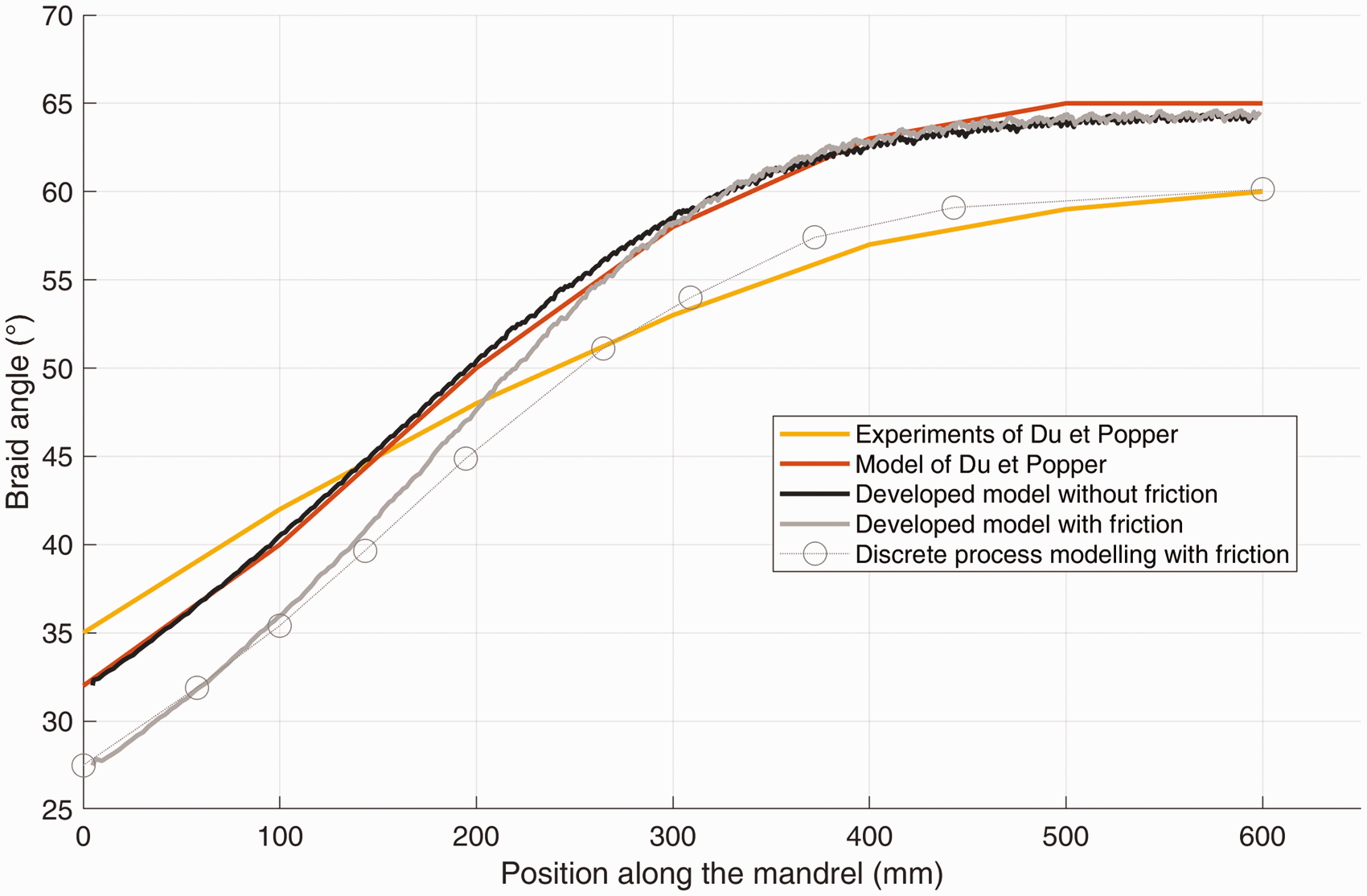
Braid angle along the mandrel form experimental measurements, from the model of Du and Popper 1 and braid angle predicted using the presented model.
The various curves can be analyzed and discussed successively. First, considering the experimental measurements, it can be observed that the braid angles increase to reach a stationary value which corresponds to the stabilization of the convergence zone length. Comparing the experimental results with the results of the model of Du and Popper, for braided length larger than 150 mm, the angles predicted with the geometrical method are larger than the experimentally obtained angles. This result is in good agreement with other results from the literature. 6 However, at the beginning of the mandrel, measured angles are larger than the predicted ones, which can hardly be explained, except by considering experimental difficulties in the experiment of Du and Popper 1 to obtain both the desired initial braid angle and the desired out of steady-state convergence zone length. The measured braid angles at the beginning of the mandrel should therefore be considered with caution. Considering the curve obtained using the presented model without friction, it can be observed that it features a very similar evolution as the model of Du and Popper. Additionally, the comparison of the evolution of the convergence zone length along time using data from Du and Popper 1 have revealed also a very similar evolution for both models as well as with the experimental values. The similarity of the results of the two models can be on one hand explained by the fact that, in both models, the friction is neglected, inducing straight yarns in the convergence zone. But this result demonstrates also, on the other hand, the capacity of the deposition algorithm to realize properly the braid deposition. Considering the curve obtained with the current model with friction, two major observations can be realized. It can be first noticed that at the beginning of braiding, the predicted braid angle is 5° smaller than the theoretical angle. The same trend has been reported by Zhang et al. using the model presented in Zhang et al.: 6 for a fixed length of convergence zone, implementing friction in the model reduces the braid angle compared to the braid angle obtained from a geometrical model. This validation regarding the work presented in Zhang et al., 6 as well as the observations on the direction of the friction forces realized in ‘Friction forces’ section validate the implemented friction model. It can further be observed that, along the mandrel, the difference in terms of braid angle between the results with and without friction reduces until the two curves overlap. This convergence of the curves has been obtained for various values of friction coefficients and is surprising regarding the analytical works presented in the literature in which friction has been reported as the major physical phenomenon allowing an accurate prediction of the braid angle.6,7 However, as both friction and deposition implemented in the current model have been validated, the evolution of the curve should be trusted and deeper investigated. In this sense, investigations can be realized on the evolution of the convergence zone length presented in Figure 15.
Length of the convergence zone versus fell front position for the model with and without friction.
It can be observed in Figure 15 that the convergence zone length reduces faster for the model treating friction than for the frictionless model (and for the experimental measurements as frictionless model and experimental results have been shown to evaluate similarly). This result is also in good agreement with the literature as van Ravenhorst and Akkerman 7 have modelled and observed experimentally that for constant braid angles at the fell point, the length of the convergence zone reduces when friction forces increase. These results and comparisons pushes thus aside the possibility of a mistake in the modelling of the process but tends to highlight the fact that a physical phenomenon is not considered here. This phenomenon would prevent, in real braiding, the length of the convergence zone to reduce as it is predicted by the presented results. This phenomenon could be yarn-yarn lateral interactions and squeezing in jamming braiding conditions. The assumption of a missing physical phenomenon is confirmed by the dotted curve which has been obtained by using discrete lengths of convergence zone, corresponding to the theoretical and measured ones. For each discrete length of convergence zone, the value of the braid angle at deposition has been calculated. As it can be observed, when the appropriate length of convergence zone is used, the predicted braid angles using friction are in much better agreement with the experimental values. Thus, assuming that the length of the convergence zone could be predicted accurately thanks to the introduction of additional physical mechanisms in the model, predictions of the deposed angles would be in much better agreement with the experiments. To conclude, the identification, formulation and implementation of the additional physical phenomenon maintaining the length of the convergence zone close to the one observed experimentally appears therefore to be a necessary future implementation in order to enable an accurate simulation of continuous braid formation and deposition.
Braid deposition in non-axisymmetric conditions
A second investigation has been conducted in order to evaluate quantitatively the capabilities of the model in non-axisymmetric conditions. For this purpose, experimental results have been taken from the work of Kessels and Akkerman. 2 In this article, a 1800 mm long mandrel featuring along the first 800 mm a square cross section, a transition region of 200 mm and a circular cross section along the final 800 mm is driven through the circular ring of a braiding machine. The particularity of the test is that the axis of the mandrel is parallel to the axis of the braiding machine but that it features a radial offset. Table 6 summarizes the process parameters used for the experiments.
Process and simulation parameters corresponding to the experiment of Kessels and Akkerman 2 .
First simulations with a square mandrel have highlighted the fact that the method allows generating the braid until the first contact with the mandrel is reached (Figure 12). As highlighted in ‘Non-axisymmetric braiding conditions’ subsection limitations of the method are then encountered due to the yarn-mandrel interactions at the edges of the mandrel. For this reason, the simulations conducted to compare with the experimental results is realized with a purely cylindrical mandrel featuring the same offset as in the experiments. Braiding is simulated with and without friction using continuous deposition. A 1200 mm braiding length allowed reaching stationary braiding. Figure 16 presents the aspect of the braid predicted using friction at the end of the simulation.
Aspect of the non-axisymmetric braid at the end of braiding with friction using parameters of Table 6 (x, y and z axes are expressed in mm).
In Figure 16, the offset of the mandrel can be well recognized (the axis of the braiding machine is located on the x-axis). Additionally the non-axisymmetric geometry of the convergence zone can be noticed. Finally the slightly curved path of the yarns in the convergence zone is a noticeable effect of the friction. These qualitative observations confirm the ability of the method to treat braiding and deposition in non-axisymmetric configurations. Additionally, quantitative investigations can be realized. Experimental results are extracted from Figure 8 in Kessels and Akkerman:
2
the average braid angle over the steady state braiding region of the mandrel (last 400 mm of the circular cross section) is taken as reference. For the values of the simulation, the braid angle of the clockwise rotating yarns at the position 1150 mm (in the steady state braiding region) on the mandrel are reported. Figure 17 presents the value of the braiding angle obtained from the model and calculated using equation (17). Some specific radial positions are highlighted on the mandrel (−90°, 0°, 90° and 180° in the -
Distribution of the braid angle around the mandrel at the axial position 1150 mm and definition of the angle β on the convergence zone obtained with friction.
Comparison of experimental results and model of Kessels and Akkerman 2 with the developed model.
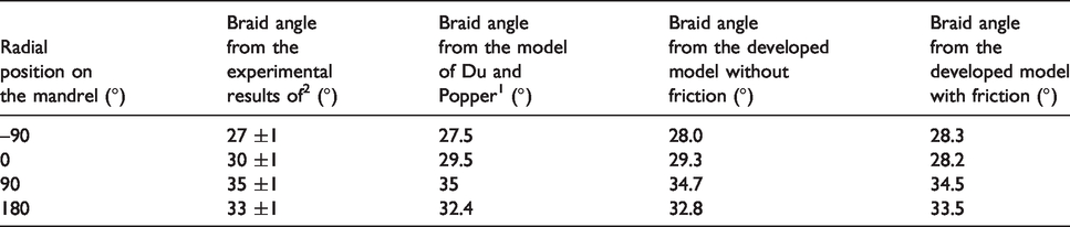
It can be observed in Figure 17 that the introduction of friction has generated a rotation of the angle distribution around the mandrel of about 10° to 20° without changing significantly the amplitude of the predicted angles compared to the frictionless results. The values of angles obtained by the model and reported in Table 7, are within the range of the experimental results obtained by Kessels and Akkerman, 2 with only minor deviations for the 90° and the 0° position of the simulation with friction which lay respectively 0.3° and 0.8° outside of the measured braid angle range. It can be furthermore noticed, that the differences between experimental and modelling braid angles are, in this case, not as significant as in the experiment of Du and Popper. In absence of details on the frictional properties of the yarns used in Kessels and Akkerman, 2 it is difficult to determine a clear explanation. This could be due to a low yarn-yarn friction leading to a braiding configuration near to the frictionless case or less lateral yarn-yarn interactions, (because of the small braiding angle of approximately 30°), leading to a convergence zone length in agreement with the one obtained by the model with friction. Nevertheless these results demonstrates quantitatively the ability of the model to treat non-axisymmetric overbraiding.
Conclusion
In this article, a new mechanically enhanced kinematic modelling method for the overbraiding process is proposed. It is based on an analytical modelling of the convergence zone and the use of a numerical method for the calculation. The ability of the method to treat important features of the process (generation of a desired braiding pattern, implementation of yarn-yarn friction, treatment of non-axisymmetric overbraiding in certain conditions) has been presented and validated. In the final section, simulations of deposition have been realized and compared with experimental results from the literature. The presented model proposes various improvements compared to the previous geometrical1,2 but also compared to analytical mechanical models of the literature6,7 as the process is modelled without symmetry assumption and enables the study of the time dependent evolutions of the braid angle along deposition on the mandrel. Furthermore, the model enables the decoupled implementation of various physics (normal yarn-yarn interactions, friction, etc) with the desired laws. This decoupling enabled to highlight the fact that friction is not the only mechanism generating discrepancies in terms of braid angles between experiment and geometrical predictions. Other physical mechanisms as lateral yarn-yarn interactions in jammed configurations seems to play a significant role and should be further investigated in the future. Finally, for equivalent braiding process parameters, the developed numerical approach has been shown to model the deposition of 450 mm of braid on a cylindrical mandrel more than 37 times faster than the most recent FEM models. 11 Because of its ability to treat non-axisymmetric braiding conditions, its flexibility in terms of implemented physics and its numerical calculation efficiency, it appears therefore that the presented method is very promising for the future braiding simulation of industrial parts. In order to reach this goal, future developments will need to focus on the implementation of yarn-ring and yarn-mandrel interactions. Additional physical mechanisms as lateral yarn-yarn interactions in jamming conditions should be also implemented in order to increase the accuracy of the technique. The flexibility of the method could also be used to investigate quantitatively the randomness of the process by introducing variability; for example by associating a different value of friction coefficients to each yarn-yarn contact point. Ultimately, in order to ease the industrial use of the model, a user-friendly software should be developed, as well as interfaces with commercial FEM codes to realize mechanical modelling of the composite parts containing the braided reinforcements.
Footnotes
Declaration of Conflicting Interests
The author(s) declared no potential conflicts of interest with respect to the research, authorship, and/or publication of this article.
Funding
The author(s) disclosed receipt of the following financial support for the research, authorship, and/or publication of this article: The authors would like to acknowledge the funding provided by the AIF-Forschungsvereinigung in the frame of the IGF project Nr. 19679 N.