Microstructural exploration of a carbon nanotube yarn reinforced composite using a peridynamic approach

Abstract

A framework using peridynamic theory is developed and demonstrated for deformation and failure analysis of carbon nanotube (CNT) yarn-based structural composites. Experimental work involved tension testing of a CNT yarn/polymer composite resulting in stress–strain response up to and including failure. The as-prepared specimen was characterized using x-ray micro computed tomography (CT), which was then converted into voxel-based data with CNT yarn, polymer, and void phases as well as surface undulation. A Density-Based Spatial Clustering of Applications with Noise algorithm was applied to detect and quantify the clusters of voids, of CNT-rich, and of resin-rich regions. The voxel data, with all microstructural details, were used in peridynamic simulations. These demonstrate the critical roles of resin and void clusters and surface undulation in fracture initiation and propagation. Additional analysis was performed to construct probability density functions (PDFs) of different phases (yarn, resin, and void) with the goal of constructing synthetic virtual composite specimens. The synthetically reconstructed peridynamic models correctly captured the experimental stress–strain response. The similarities and differences between the failure (initiation and propagation) behaviors predicted by x-ray CT-based and PDF-based peridynamic model simulations are presented in detail and discussed.

Keywords

Carbon nanotubes non-local peridynamics fracture damage Carbon nanotube-based composite

Introduction

Carbon nanotubes (CNTs) have been studied extensively for decades.¹ Although the measured nanoscale stiffness of CNTs has been reported on the order of 1 TPa^2–4 and the strength in the range of 50–100 GPa,^4,5 their envisioned use in the creation of a bulk scale composite with such properties has not been fully realized. One of the current challenges facing the aerospace structures community is to carry these nanoscale properties to the macroscale. A potential solution to this challenge is the development of CNT macro assemblages, in particular, CNT yarn. Recently developed manufacturing techniques have made CNT macro assemblages more readily available for aerospace applications.⁶

In comparison to carbon-fiber composites, CNT yarn-based composites have not been fully characterized. This lack of characterization can be traced back to advances in processing control. The large variety of processing parameters and post-processing procedures lead to a great diversity of microstructures. Experimental testing of each unique microstructural realization is simply not feasible. The expensive and time-consuming nature of experimental testing necessitates the advancement of simulation methodologies that can incorporate microstructural details. It is believed that such simulations could provide feedback to both synthesis and processing researchers, allowing a more targeted search for desirable structures.

Predicting and understanding the failure of materials has long been a challenging endeavor. Peridynamics (PD), first introduced in 2000,⁷ is a nonlocal continuum based theory that has proven to be successful in capturing the failure and fracture behavior of a wide variety of material systems. Over the years, the failure prediction capabilities of PD theory have been demonstrated on glass,^8–10 metal,¹¹ and carbon-fiber composite^12,13 material systems. The theory is particularly adept at simulating failure in these material systems because of its integral formulation which, unlike its differential counterpart, does not give rise to the mathematical singularities associated with fracture.⁷

In recent years, various PD approaches have been developed for carbon-fiber reinforced polymer composites.^13–15 Only a few researchers have explored the application of PD to CNT composites. In the early work,¹⁶ Bobaru et al. developed a 3D PD framework for carbon nanofiber networks and CNT composites. The authors demonstrated the ability of PD to capture complex failure behavior associated with the stretching of a fiber network and CNT pullout. Rahman et al. used a hierarchical multiscale modeling approach to link atomistic simulations with a coarsened state-based PD model.¹⁷ In that work, the researchers explored deformation mechanisms associated with carbon nanofibers. More recent work¹⁸ combined bond-based PD and Monte Carlo simulations to predict the mechanical properties for CNT-based nanocomposites.

A major distinction between previous PD CNT frameworks and the one proposed in this work is the length scale at which simulations are performed. In all of the above work, simulations were performed at the CNT/nanofiber length scale (nanometers). In the current work, the simulation domain is increased and simulations are performed at the CNT yarn length scale (micrometers).

We aim to provide a systematic approach to incorporate microstructural information into the simulation process. In the current work, x-ray computed tomography (CT) is used to develop a simulation grid containing constituent level information. The composite microstructure is characterized using statistical and data clustering algorithms. A novel peridynamic approach for simulating CNT yarn composites has been developed to accurately capture the failure morphology and to investigate its origins. Finally, a framework was developed for creating synthetic microstructures through the use of probability density functions.

Experimental work

In the previous work by Kim et al.,¹⁹ unidirectional CNT yarn polymer composites were fabricated from highly densified CNT yarns (provided by Nanocomp Technologies, Inc.). Each yarn was composed of 4 plies of CNT roving. The 4 ply yarn has an irregular shape measuring an average of approximately 250 μm in diameter. Cyanate ester (RS-16) resin from Tencate Advanced Composites was diluted with methyl ethyl ketone (MEK) to a 65 wt. % MEK solution. A 100 to 9 mix ratio between resin solution and curing agent was used. The resin solution was applied to the CNT yarns by a wet winding method using a custom-built filament winder, with an applied winding tension of 13.34 N.⁶ The CNT yarn was passed through a resin bath followed by direct winding onto a custom-made solid aluminum plate (width of 15.24 cm and height of 10.16 cm) as shown in Figure 1. The as-wound materials were sandwiched between two steel plates and then cured with a 4 h hold at 113° C followed by a 1.5 h hold at 135° C under a cure pressure of 10.34 MPa. The final composite panel dimensions were 10.16 cm (height) × 2.54 cm (width) × 383 μm (thickness). The resin and void contents of the composite were 19 wt. % and 2%, respectively.

Tensile properties of tabbed unidirectional c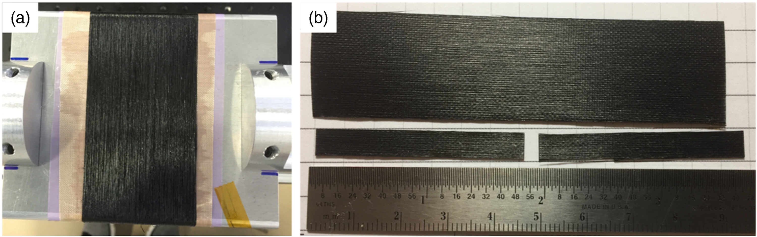omposite specimens (10 cm (height) × 0.5 cm (width)) were measured using an MTS-858 test stand equipped with a laser extensometer and pneumatic grips. P180 sandpapers were glued to the ends of the composite specimens using cyanoacrylate. A crosshead speed of 0.5 mm/min was used during the test. Table 1 lists the material properties associated with the yarn, resin and composite. The diameter variations found in the CNT yarn prevent accurate measurement of yarn properties in volume-based units. Instead, linear density-based tex units are used (1 tex = 1 g/km) for the reported specific strengths and moduli, 1 N/tex = 1 GPa/(g/cm³).

Table 1.

Material properties of carbon nanotube yarn polymer composite.

Material	Density g/cm³	Specific strength MPa/(g/cm³)	Specific modulus GPa/(g/cm³)
Yarn units	tex	N/tex	N/tex
Resin: Cyanate ester^a	1.19	67	2.5
Yarn: 4 ply^a	26.89	1.63	96.3
Composite	1.14	1130	72.3

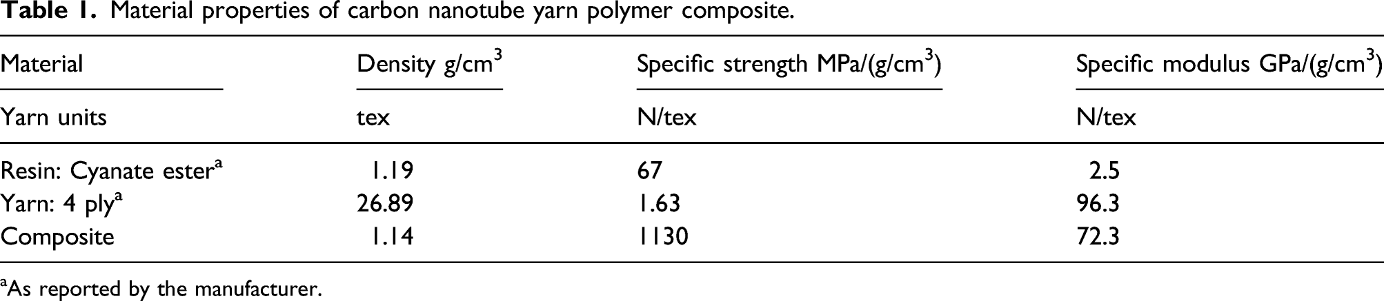
^aAs reported by the manufacturer.

High resolution nondestructive evaluation of as-prepared unidirectional CNT yarn/polymer composites was conducted using a micro focus x-ray computed tomography (CT) system (Nikon Metrology) with a maximum resolution of 5 μm and magnification of up to 160×. A Perkin-Elmer 16-bit amorphous silicon digital detector with a 2000 x 2000 pixel array was used to collect radiographs at each rotation angle as the x-ray path intersected the sample (360° in 0.11° increments). The three-dimensional reconstruction of the collected radiographs produced tomographic data that could be viewed along any plane in the sample volume.

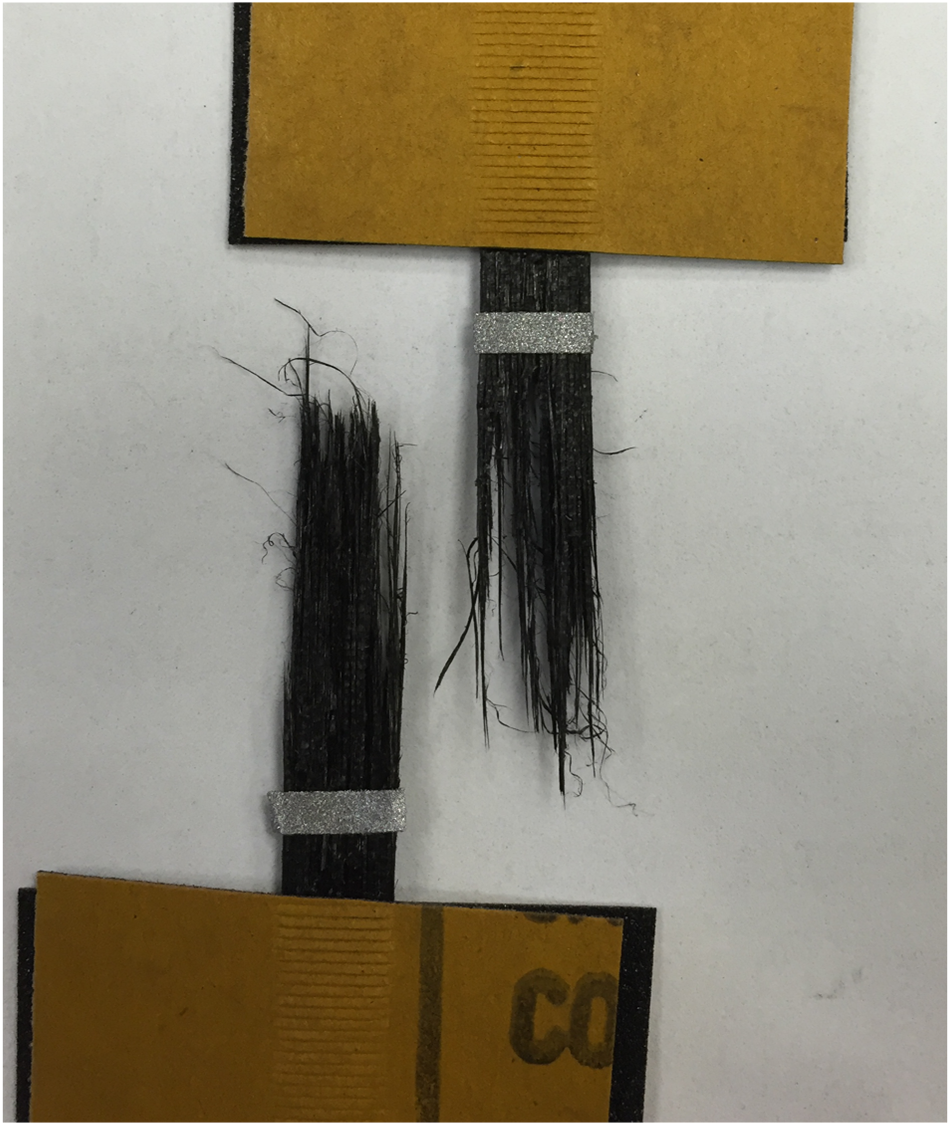
An experimentally obtained, representative stress–strain curve is presented in Figure 2. The initially observed stress stiffening is attributed to the elimination of slack and an increase in alignment of the CNT yarns as the load is applied. The softening behavior observed prior to failure is attributed to partial damage to the yarns before the complete failure of the specimen or originated from the typical mechanical response of CNT assemblies such as yarns and sheets. Figure 3 shows the fully failed specimen. The fully failed specimen shows failure in multiple locations of the specimen and a yarn pullout failure morphology.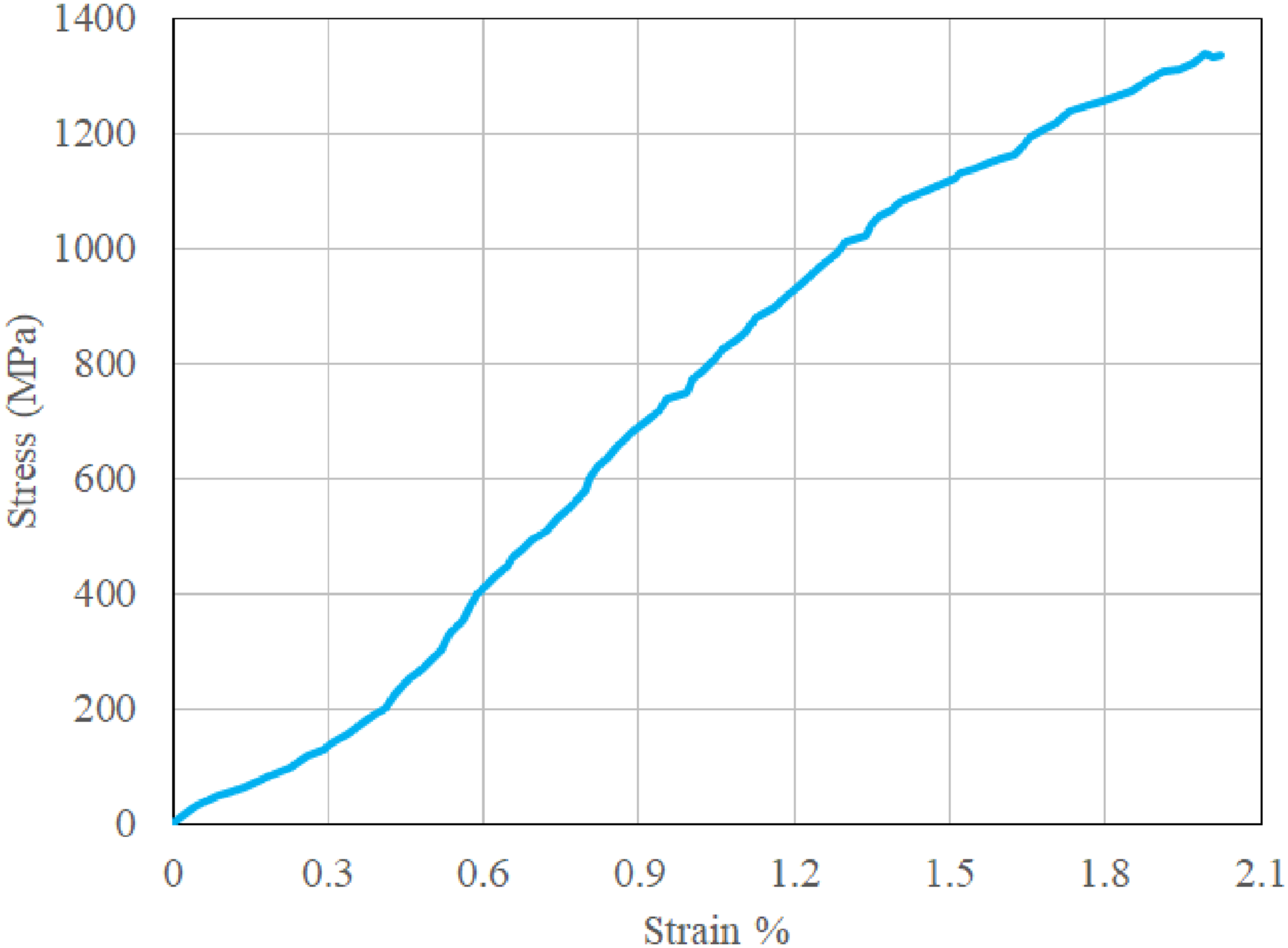

Microstructure characterization

A procedure was developed to convert the x-ray CT bitmap (BMP) images into a PD simulation grid to incorporate structural features in the model. Features associated with the grids were then characterized using simple statistical methods and data clustering algorithms.

X-ray CT imaging

The reconstruction of the CNT yarn composite sample characterized using micro x-ray CT produced a data set with dimensions of 2000 (width) × 722 (height) × 1999 (length) pixels and a reconstructed pixel resolution of approximately 3.6 μm in each direction. This data set served as the foundation for the PD simulation grid. Figure 4 presents a gray scale cross-sectional view of the composite obtained after the scanning process and demonstrates several directly observable features such as surface undulation, resin-rich regions, and porosity.

Thresholding process

Data obtained from the x-ray CT was post-processed using ImageJ²⁰ and converted from its native file type into a series of BMP images. Python scripts were used to segment these BMP images based upon pixel gray scale value. Following the work of Kim et al.,¹⁹ the threshold set point was obtained in ImageJ through manual adjustment and visualization of the porosity. During thresholding, gray scale values below the set point were discarded while higher values were kept. This initial thresholding effectively separated the foreground and background of each BMP slice, whereas internally discarded pixels indicated the presence of voids.

The retained pixels became the PD simulation grid. Figure 5 compares a single BMP slice against its segmented counterpart. For visualization purposes, lighter shades of gray coming from the BMP image are shown in the PD grid as orange/red colors, while darker shades of gray are green/blue in color.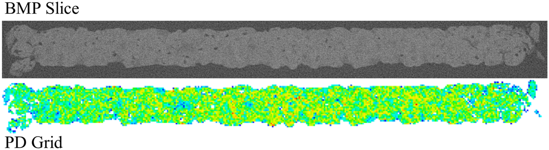

The final step in the grid generation process was to assign pixels as either CNT yarn or resin material. This was accomplished using a second threshold. The value of the secondary threshold was allowed to vary for each individual BMP slice. This variability arises as a result of contrast differences within the data set and is an artifact of the x-ray CT. To account for the variation in contrast, a series of thresholds were iterated through for each slice. The threshold set point was optimized by minimizing the difference between the calculated and experimentally measured resin volume fraction. Figure 6 shows a cross-sectional view after the thresholding procedures. In this figure, blue and red squares represent yarn and resin material points, respectively.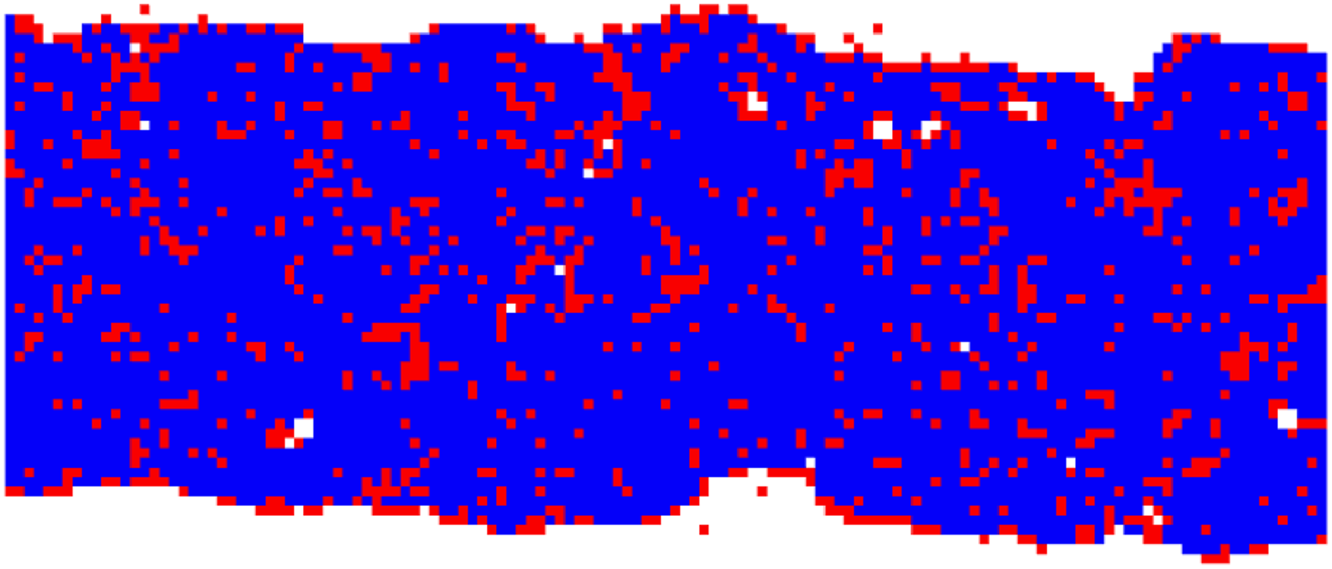

The x-ray CT was partitioned into four quadrants and four separate cells were created at 7.27 micrometer grid spacing. This permitted a high level of microstructural detail without exceeding available computational resources. Figure 7(a) shows the locations of the cells on the x-ray CT domain. Cells were selected to exclude any boundary effects and were positioned to obtain a representative sampling of the entire specimen. It is worth noting that the current study is not a micromechanics analysis²¹ in that it is not making predictions of homogenized bulk properties based on multi-phase microstructures; for a peridynamic approach focusing on micromechanics analysis, see Ref. 22. Each cell has dimensions of approximately 1 mm × 1 mm × 0.4 mm and contains approximately 900 thousand material points with a grid spacing of 7.27 μm. An isometric view of Cell 1 is provided in Figure 7(b), where red and blue voxels represent resin and yarn material, respectively. Figure 7(c) shows the same isometric view of the cell, but colored by z-coordinate location. The alternating sequence of coloring on the top surface demonstrates the surface undulation present in the composite. Finally, Figure 7(d) shows a cross-sectional view of the composite. From this orientation, one can clearly see clustering of the resin material.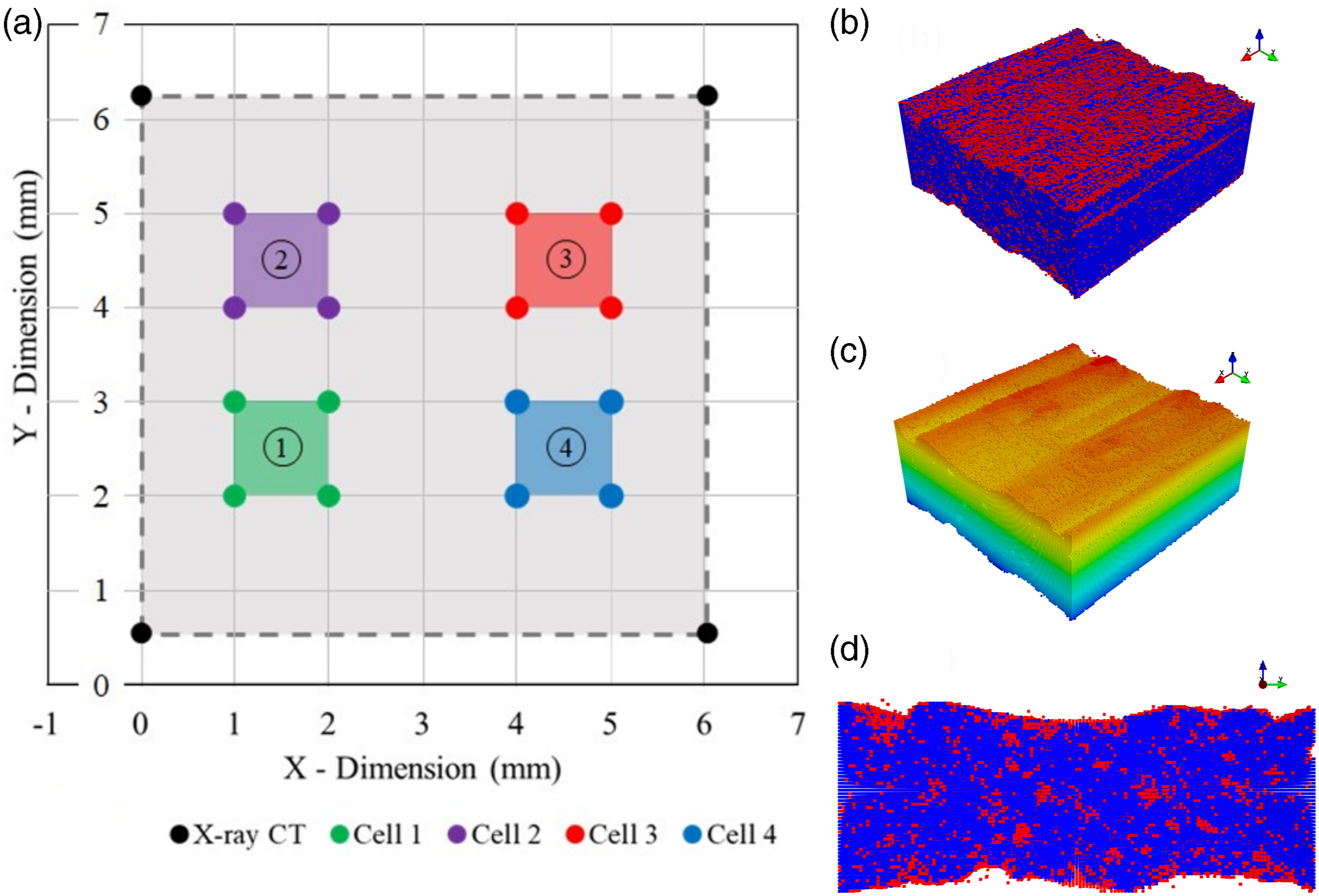

After the generation process, the structural features of each cell were characterized. The features under consideration include: the number of material points, the average thickness, the resin volume fraction, and the void fraction. Complete details of the characterization are provided in Supplementary Material Appendix B.

Quantification of resin and void clusters

Two distinct algorithms were used to identify and characterize the groupings (clusters) of resin/void material on each individual slice. After assignment of resin/void material points, a K-nearest neighbors algorithm²³ was applied to detect the resin/void material points. The K-nearest neighbors routine identifies the resin/void material points to be placed into separate clusters, and performs an initial removal of noise from the data set. It is worth noting that it does not separate the points into clusters. Subsequently, a data clustering algorithm called Density Based Spatial Clustering of Applications with Noise (DBSCAN) was applied to detect and quantify individual void/resin clusters. This algorithm, first presented by Ester et al. in Ref. 24, is well suited for this task because of its ability to discover clusters of arbitrary shape and its ability to distinguish “noise” within the data set.

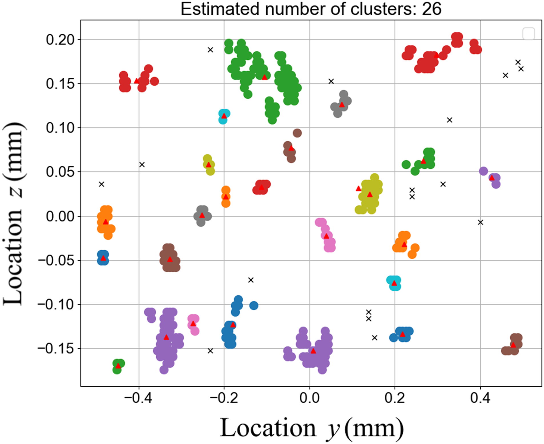
The clustering process is demonstrated by considering an example slice shown in Figure 8 with the yarn, resin, and void material points. In this instance, first the K-nearest then the DBSCAN algorithm was applied to identify the resin clusters of the slice (red points in Figure 8). Figure 9 shows the result of the process itself. In this instance, the algorithm detected 26 different resin clusters of various sizes. For visualization, each uniquely classified resin cluster is assigned a different color and the center of the cluster is shown using a red triangle. Also shown by the black crosses are resin material points considered by the algorithm to be “noise” and therefore not associated with any of the clusters. This procedure is performed on every BMP slice of the data and the resulting information about resin and void clusters is stored.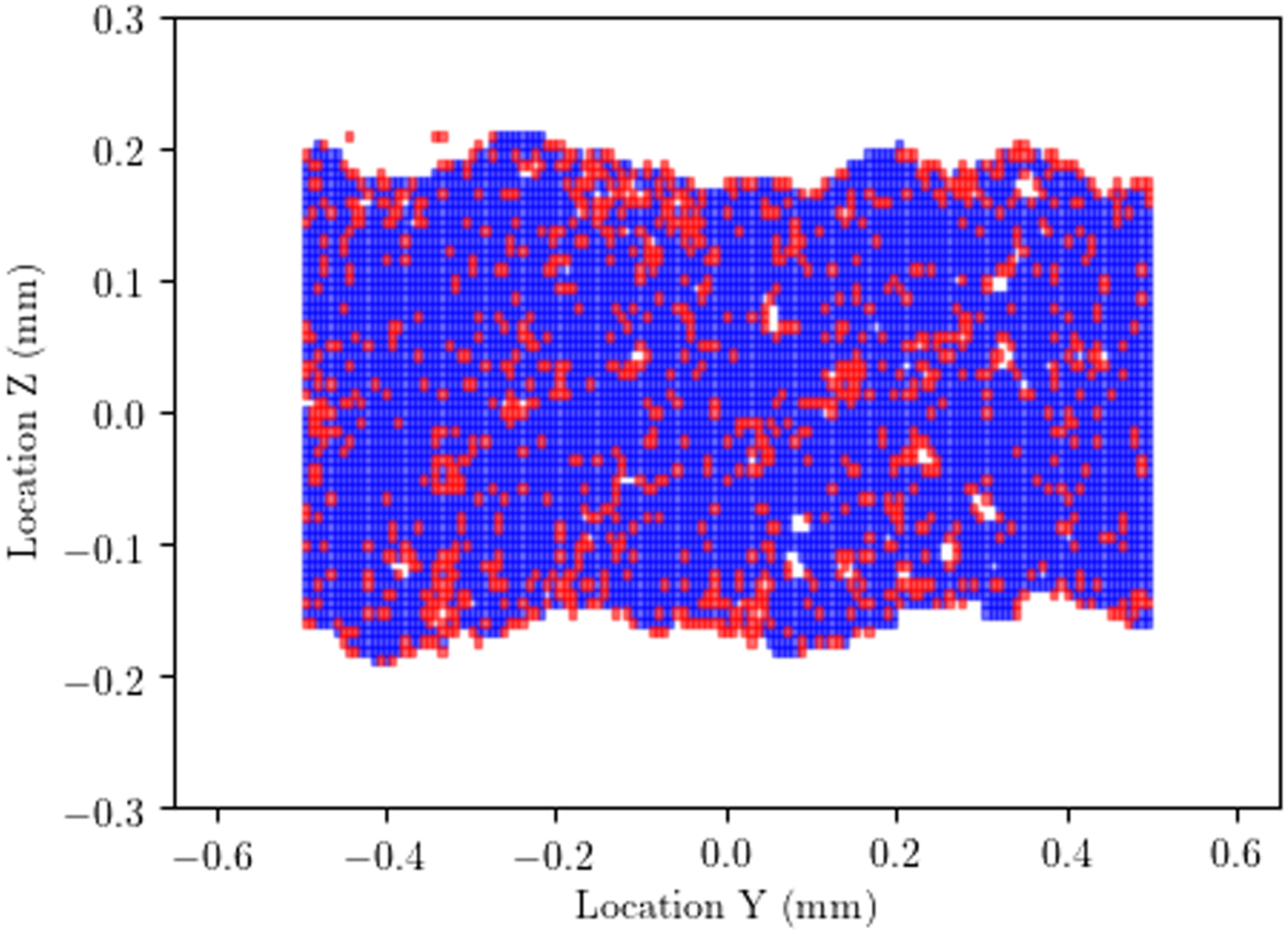

Peridynamic modeling approach

Peridynamic (PD) theory is a nonlocal reformulation of classical continuum mechanics (CCM) which removes singularities arising from geometric discontinuities such as cracks or material interfaces. This is achieved by reformulating the CCM equation of motion into an integral equivalent form. In this nonlocal theory, a material point interacts with other material points within a prescribed finite radius, termed the horizon. The nonlocal equation of motion, derived in Ref. 12,25,26, for a material point $x$ at time $t$ can be written in the following form;

\begin{matrix} ρ \frac{\partial^{2} u}{\partial t^{2}} = \int_{H} f (u' - u, x' - x, t) d H + b (x, t) \end{matrix}

(1)

where

ρ

and b denote the mass density and body force density vectors, respectively. In equation (1),

H

is the neighborhood of point x^′ in which the members of

x^{'}

belong. The displacement vector field u at point x^′ results from the interaction between the material point x^′ and points x^′ due to the pairwise force response function

f (u^{'} - u, x^{'} - x, t)

. In this equation, the divergence of the stress tensor from CCM has been replaced by an integral equivalent form. The integration is performed over volume defined by the horizon, and is typically represented by the variable

δ

. The horizon is a nonlocal parameter and suggests that a material point is influenced by all material points within its horizon, in addition to its nearest neighbors. An overview of PD theory is provided in Supplementary Material Appendix C, and is described in the literature with more details.^7,12,26 In this study, bond-based PD formulation is utilized, which results in a Poisson’s ratio value of 0.25 for homogenous deformations of linear isotropic materials.^7,27 This restriction may introduce varying degrees of inaccuracies to the analysis depending on the specifics of the problem being considered, and properties of the constituent materials. The composite system in this study is heterogenous in a highly irregular manner, providing a multitude of failure initiation sites. As the results demonstrate, surface irregularities and clusters of voids and resin play critical roles in initiation and propagation of failure and fracture. Considering the Poisson’s ratio for common unidirectional carbon-fiber polymer composites range between 0.2 and 0.4, the influence of the inaccuracy due to the Poisson’s ratio limitation on the failure behavior of the composite specimen considered in this study is deemed minimal.

Several modifications to the traditional bond-based PD method were needed to properly simulate the explicit yarn and resin material regions extracted from the x-ray CT. These modifications are necessary to introduce the anisotropic material behavior of unidirectional composites. To develop anisotropy in the PD model, bonds were categorized based on material associations. Depending upon the bond type categorization, bonds were given different constitutive properties.

Bond types

Based on material association (yarn/resin) and alignment, several bond types were considered. Table 2 shows the relationship between material association, alignment and behavior for these various bond types. The start and end point material association of a bond are given in the second and third column, respectively. The first set of bond type variations, labeled (1a–1c), are considered yarn–yarn bonds. For these three variations, alignment is an important consideration and is given in the fourth column. The first variation, 1a, is a yarn–yarn bond that is perfectly aligned with the yarn direction. In this scenario, the bond’s behavior is governed by the yarn bond constant. The second variation, 1b, is a yarn–yarn bond that is oriented perpendicular to the yarn direction. In this instance, the bond behavior is governed by the resin bond constant as the yarns are only connected to each other through resin in that direction. Finally, the third variation is a bond that is oriented in between the parallel and perpendicular directions. For this scenario, the bonds have a material constant in between the yarn and resin bond constant and are governed by the off-axis modulus function.

Table 2.

Relationship between material association, alignment, and behavior for various bonds.

Bond type	Material point 1	Material point 2	Alignment	Behavior
1a	Yarn	Yarn	Parallel	Yarn
1b	Yarn	Yarn	Perpendicular	Resin
1c	Yarn	Yarn	Off-axis	Off-axis
2a	Yarn	Resin	NA	Interface
2b	Resin	Yarn	NA	Interface
3	Resin	Resin	NA	Resin

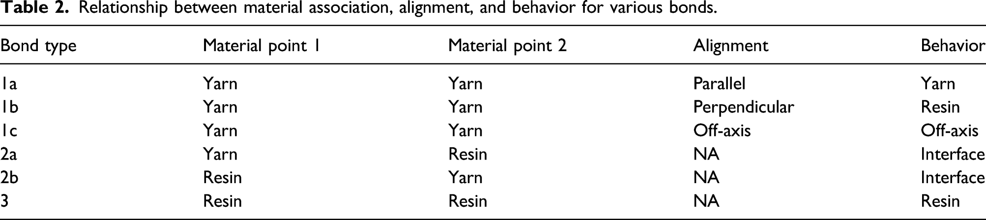
The next variations considered were bonds consisting of one resin and one yarn material point. These bonds are treated as interface bonds and do not have any direction dependent properties. While classified as interface bonds for completeness, in the current work they use the same bond constant as the resin bond. Finally, the third variation is resin–resin bonds. Like the interface bonds, they do not have any directional dependency and are governed by the resin material properties.

Figure 10 pictorially illustrates the bond types that are possible within the model and their associated behavior. In this figure, blue squares represent yarn material points and the red squares represent the resin material points. Two separate scenarios are drawn. The first scenario is a yarn point located at the center, while the second is that of a resin point located at the center. The possible interaction behaviors are shown using different colors, interface in green, resin in red, yarn in blue, and off-axis in purple.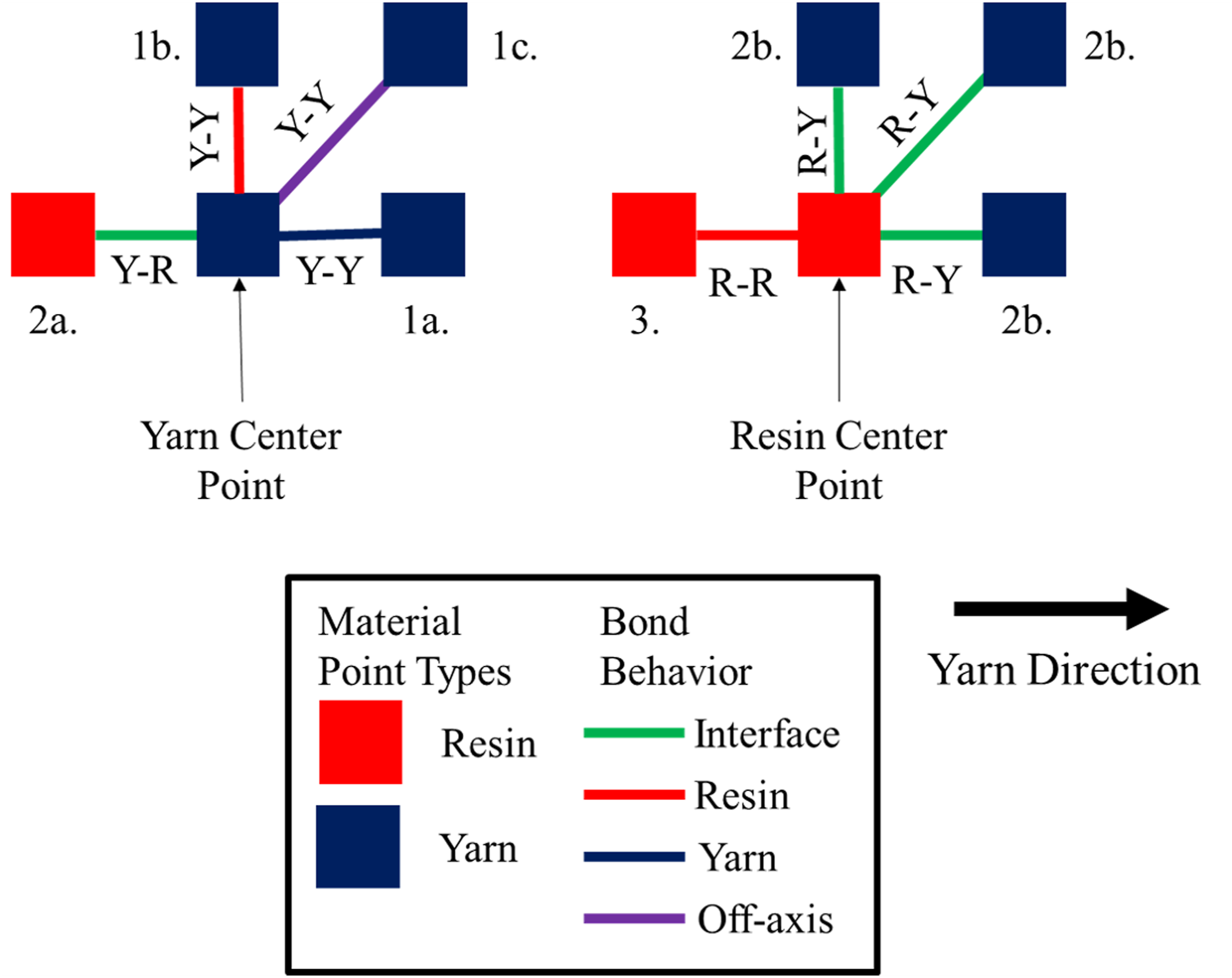

Off-Axis modulus function

Figure 11 shows the constitutive relationships associated with each bond type. For simplicity, each constitutive relationship is of a linear form and can be fully described by two material parameters: a bond constant and a critical stretch. The bond constant is the slope of the force–stretch curve while the critical stretch is a strength related parameter. The deformation of the bond may continue to a value that leads to its breakage. The stretch value at this state is called the critical stretch. The yarn constitutive relationship is given in blue and has a higher bond constant and lower critical stretch as compared to the other bond types. At the other extreme, the resin constitutive relationship, shown in red, has the lowest bond constant and the highest critical stretch. The interface constitutive relationship in green follows the resin behavior in this study. Finally, the off-axis yarn constitutive relationship in purple falls between the yarn and resin relationships. Equations (2–4) show the bond force versus stretch relationship for each bond type.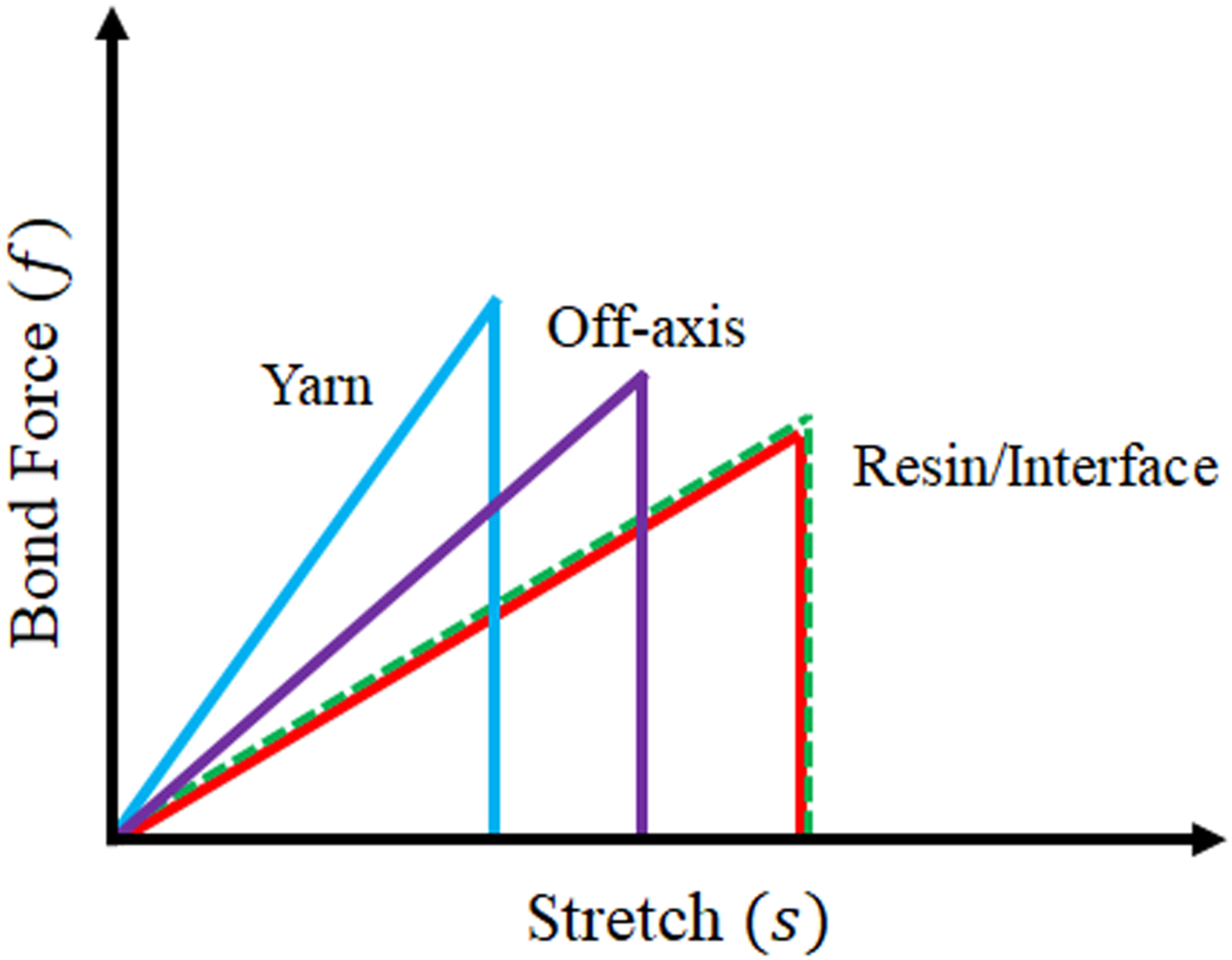

\begin{matrix} f_{y} = c_{y} s_{i} \end{matrix}

(2)

\begin{matrix} f_{r} = c_{r} s_{i} \end{matrix}

(3)

\begin{matrix} f_{o} = ϕ_{c (i)} c_{y} s_{i} \end{matrix}

(4)

The

c_{y}

and

c_{r}

constants can be determined by applying load along the yarn direction and then subsequently along the transverse direction. The composite specimen was only experimentally tested in the yarn direction so its behavior in the transverse direction is not currently known. Because transverse properties in uniaxial composites are generally matrix dominated, the transverse modulus was assumed to be that of the resin material.

The anisotropic material behavior was included in the model through the application of an off-axis function. The form of the off-axis function is given by equation (5). This Gaussian function is used to ensure that yarn bonds oriented along the loading axis are attributed yarn material properties and bonds oriented “off-axis” are assigned a reduced bond constant. A bond perpendicular to the yarn direction is attributed the ratio of resin to yarn bond constant c_r/c_y. This ensures that, upon multiplication with the yarn bond constant, the material property degrades back to the resin bond constant. Also in this equation, the variable $w$ represents the width of the Gaussian function and $θ$ is the bond angle with respect to the yarn axis.

\begin{matrix} ϕ_{c} = (1 - \frac{c_{r}}{c_{y}}) e^{- \frac{{(cos θ - 1)}^{2}}{2 w^{2}}} + \frac{c_{r}}{c_{y}} \end{matrix}

(5)

A sampling methodology was developed to find an expression for the PD elastic constants in a heterogenous domain. In this method, a statistical representation of material point families was obtained by repeatedly sampling the interior points. Statistical sampling is necessary because the composition of a material point’s family is unique and based on the x-ray CT grid generation process. Complete details of this procedure can be found in Supplementary Material Appendix C.

Simulation procedure

The experimentally generated stress–strain curve was simulated by dividing the loading curve into multiple load steps. The blue curve of Figure 12 shows the experimental stress–strain curve, while the red points show the chosen load steps for the simulation. The strain associated with each load step was converted into a displacement and applied as the boundary condition.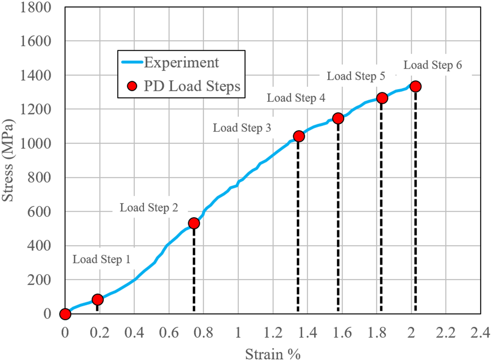

Within each load step, a dynamic relaxation procedure was followed.¹² A quasi-static solution was obtained for each load step by applying a small constant viscous damping coefficient to the velocity of each material point in the system. After equilibration, bonds were allowed to fail progressively until no further damage accumulated, after which, the next load step was entered. A complete description of the dynamic relaxation procedure can be found in Ref. 12. The engineering stress values for the peridynamic simulations were calculated based on the x-component of the total force of all the bonds crossing a plane that is parallel to y–z plane located at the half length in x-direction of the peridynamic domain, and the area of this specific plane. In this study, it is assumed that the initial cross-sectional area remains unchanged.

Within each load step, the displacement boundary condition was ramped over 10,000 timesteps. The internal force of the specimen was monitored for the duration of the simulation by placing an imaginary force plane in the middle of the tensile specimen and summing each of the bond forces crossing the plane.

PD simulation results

Peridynamic simulations used elastic properties for different bond types as explained in Bond Types, Off-Axis modulus function and Supplementary Material Appendix C. In order to model failure, each bond also has the critical stretch property that dictates the stretch value at which the bond breaks. For the resin bonds, a value of $s_{cr}^{resin} = 4.2 \times 10^{- 2}$ was used based on averaging of fracture toughness values found in literature for cyanade ester.^28–31 There is no established fracture toughness data in literature for yarns composed entirely of CNTs. The failure of CNT yarns are affected by multiple factors including CNT chirality, vacancy defects in CNTs, CNT and bundle alignment, and bundle entanglements.^32,33 Critical stretch value of $s_{cr}^{yarn} = 3 \times 10^{- 2}$ was found to be suitable for all simulations in this study. The interface bond critical stretch was calculated by following the procedure in Off-Axis Modulus Function.

Figure 13 shows the stress–strain responses for each individual cell and their comparisons to the experimental work of Kim et al.¹⁹ As expected, the heterogeneity and uniqueness of each cell gives rise to some minor fluctuations in the response. Figure 13 shows that the largest difference in the response can be observed in the failure strain. Failure of the cells is determined to occur when the internal force measured through the force plane drops to 0. Although further refinement in the load step increment is needed to determine the exact strain at failure, the first and the fourth cells fail between the 2.0% and 2.2% strain load steps, while the second and the third cells fail between the 2.2% and 2.4% strain load steps. Another observation is that unlike the experimental stress–strain curve, which exhibits a softening behavior in the stress–strain response after approximately 1.5% strain, the simulated stress–strain curves are all linear. This response can be explained by the linear-elastic constitutive relationship employed in the PD simulation approach. While the PD simulations slightly overpredict the tensile strength, an overall good agreement is observed between the experimental and numerical results.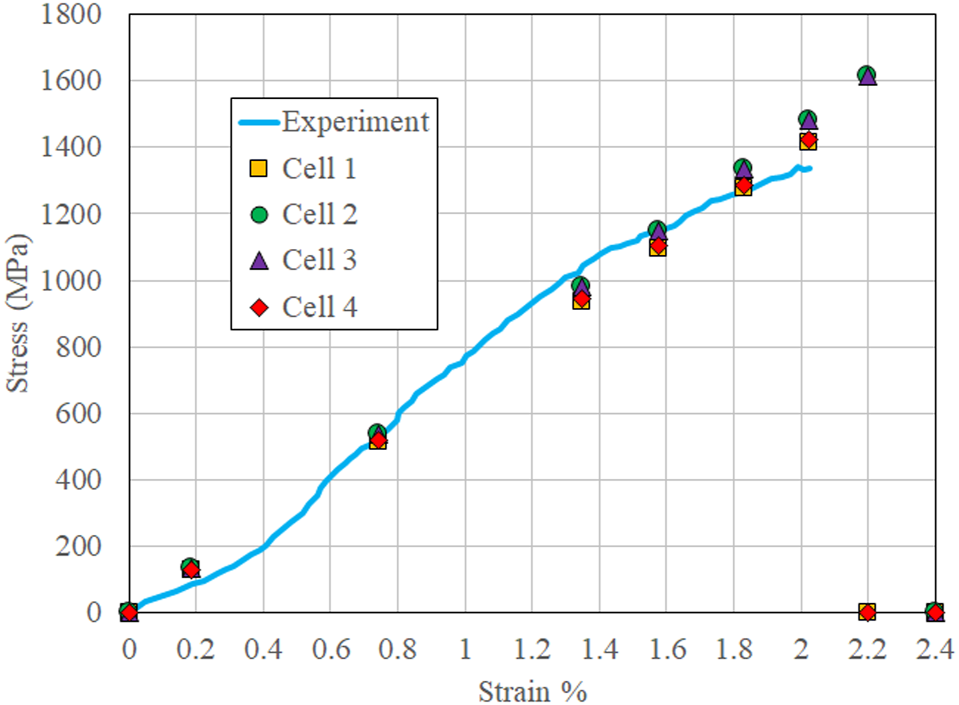

A comparison of the stress-strain simulation results with the microstructural characterization, contained in Supplementary Material Appendix B, lead to a few readily apparent trends. First, the total numbers of material points in the cells are very similar. This could be one possible explanation for the similarity in the stress–strain curves themselves. Additionally, a minor variation exists between cells 2 and 3 and cells 1 and 4 in both the total number of material points and the stiffness in the stress–strain response. Second, the two cells that fail at a higher strain %, cells 2 and 3, also have the lowest void fraction. The low void content of these cells could explain the higher failure strain and indicate that voids in the PD model influence the failure behavior. For these particular models, a ∼0.8% decrease in void fraction increases the failure strain by ∼0.2%.

Peridynamic theory is well-suited for investigating complex failure morphology. Figure 14 shows a set of damage contours in each of the four cells from three distinct perspectives with the yarn oriented along the x-direction. In this image, damage of a material point is colored on a scale ranging from 0 (blue) to 1 (red). Colors close to blue indicate less damage while colors close to red indicate a heavily damaged material point. The columns in this image show the damage in each cell. The first row shows an isometric view of the damage contours in each cell. From this orientation, only damage on the external surfaces is visible. For this reason, an internal slice of the specimen is provided in the second row. From this slice, an internal section along the yarn direction is visible. Finally, the “bottom half” in the third row shows the specimen after being sectioned at the midplane. These contours demonstrate that failures, while not the same in each cell, share some common characteristics. First, in all cases, the specimens are highly damaged on the surfaces and damage is oriented along the longitudinal (yarn) direction. Additionally, damage is present in the entirety of the specimen and is not limited to the surfaces. Overall, the damage observed in the PD simulations matches well with the experimentally observed failure as shown in Figure 3.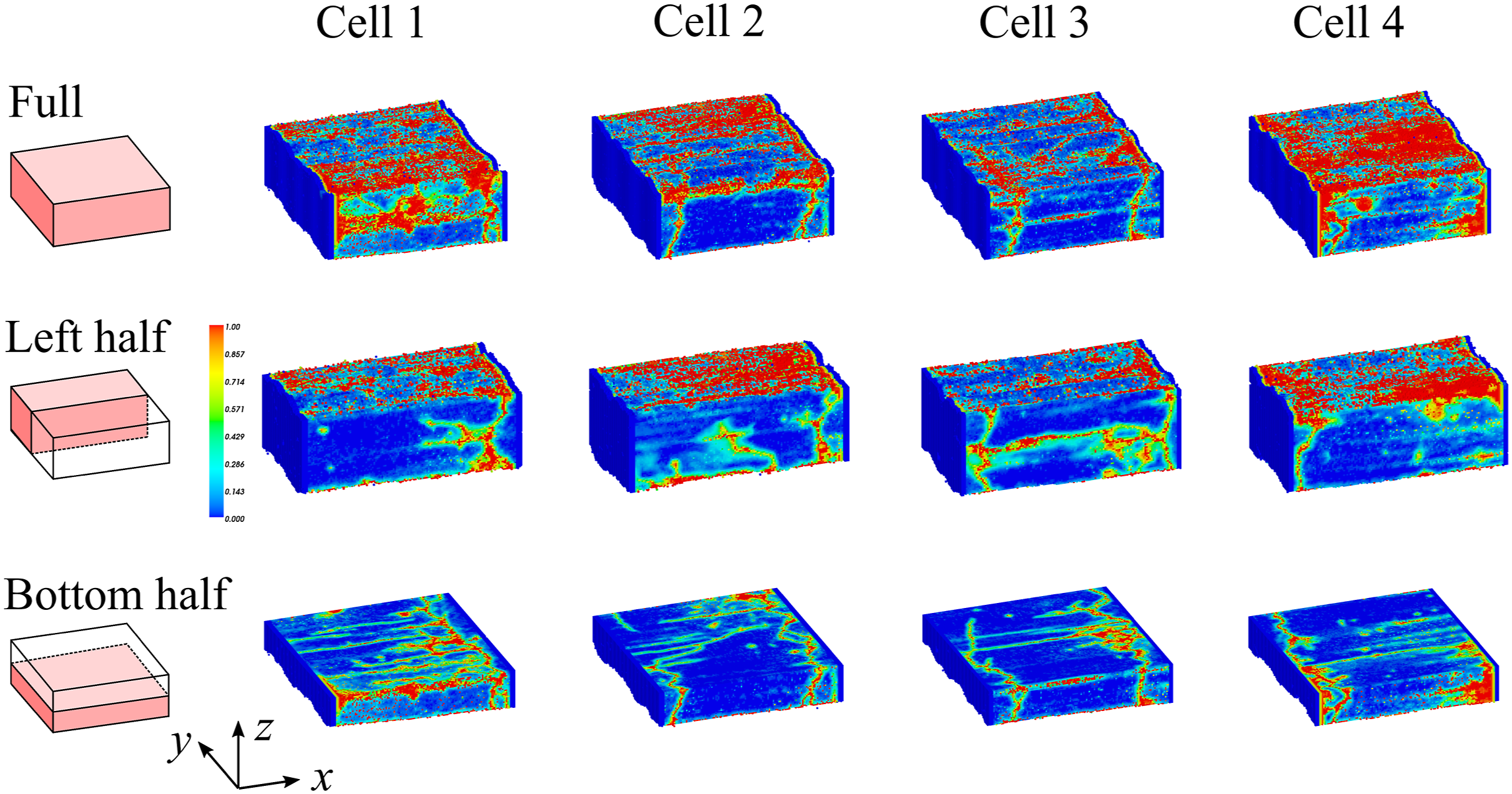

To better understand the relationship between the microstructure and the developed damage, an overlay was created for various YZ planes of the specimen with X-axis being the yarn direction. Each row of Figure 15 shows a different YZ plane, highlighted in red, of the specimen: left, middle, and right, front, middle, and back. In this orientation, yarn is perpendicular to the plane. The middle column of the figure shows the microstructure of the slice. In this image, blue voxels represent yarn, gray voxels represent resin, and white voxels represent voids. The right most column shows accumulated damage on the slice. Undamaged material points of the slice have been removed and the remainder is plotted with the color representing the intensity of damage with red indicating the most damaged areas. The left column shows an overlay of the material association and the damage. For visualization purposes, transparency was added to the image. From the overlay, i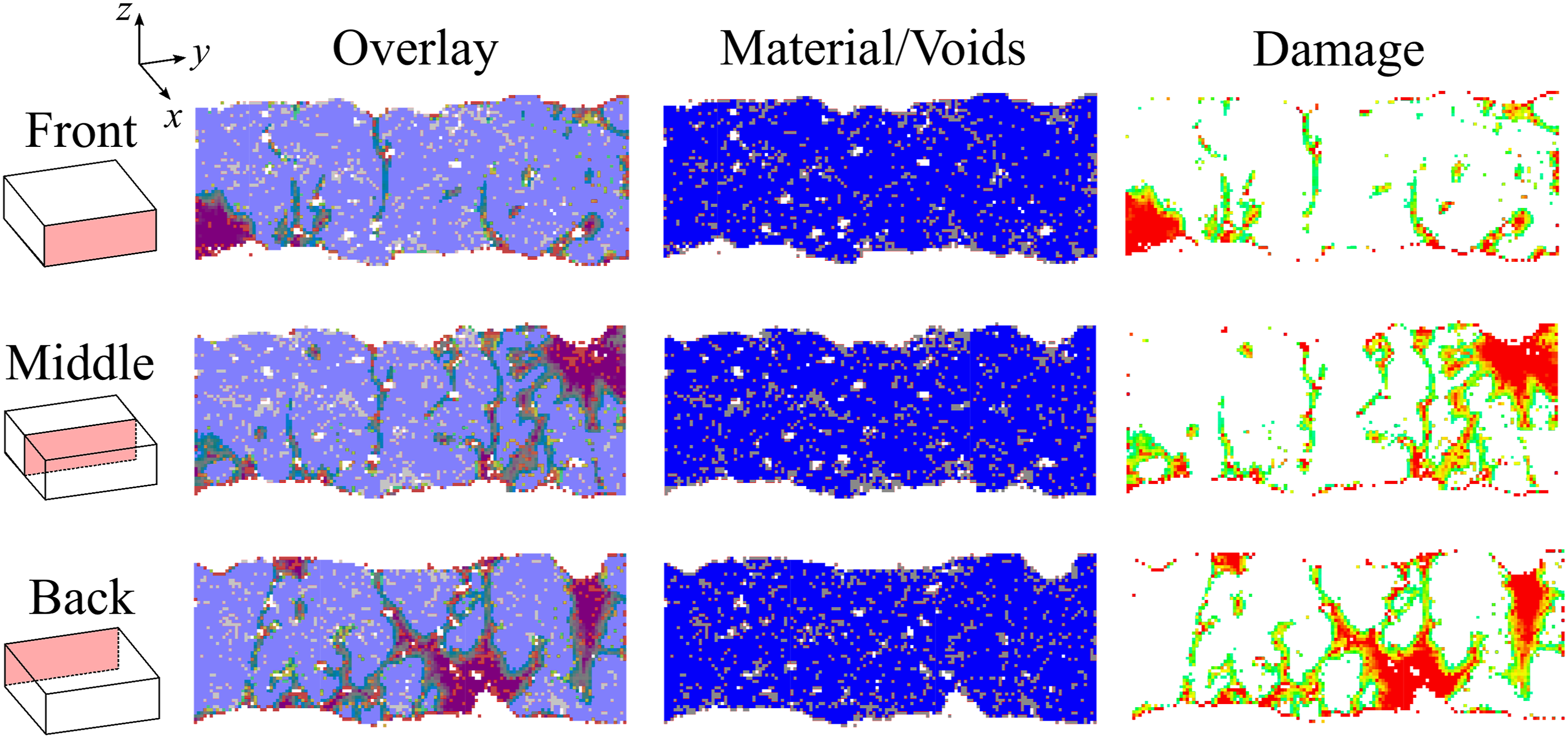t is observed that streaks of damage connect both resin and voids. Damage is observed to accumulate most around the void clusters and at the surfaces of sharp undulation. Additionally, damage is spatially located in similar locations on each slice indicating a continuity of the damage in the out-of-plane direction.

A similar set of overlays are shown in Figure 16. These figures show snapshots of the damage progression in the YZ planes. From top to bottom (1–7) the snapshots show the damage process during the final load step. The progressive nature of the failure (snapshots 1–7) occurs as a result of the load redistribution during the failure process. In the fourth row of the left column, damage is first observed in the voids closest to the surface. In the next image, damage has extended towards the surface while following the closest voids. In the middle plane, damage is observed not only at the voids closest to the surface, but also at the top right surface where there is a sharp gradient in the surface waviness. As observed in the left front plane, damage extends from the voids closest to the surface to the internal voids. Finally, in the right most back plane, there are two sharp gradients in the surface waviness. Damage initially accumulates in both of these sites (sequences 3 and 4). For completeness, damage overlays of cells 2–4 are provided in Supplementary Material Appendix E.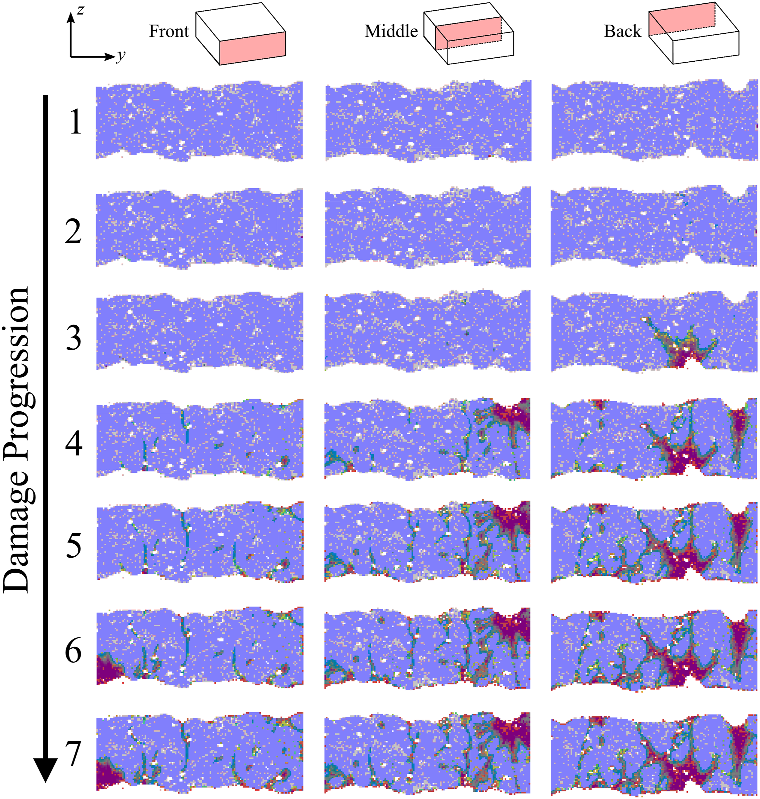

Synthetic microstructure reconstruction

For the final aspect of this work, a methodology is presented for creating synthetic microstructures that are structurally similar to the experimental sample. Such reconstruction can provide insight into the features that heavily influence the mechanical response.

Probability density functions

Synthetic reconstruction is accomplished through the representation of the microstructure as a series of probability density functions (PDFs). Using the statistical information from the characterized x-ray CT images, a PDF was created using equation (6).

\begin{matrix} p (x) = \frac{1}{\sqrt{2 π σ^{2}}} e^{- \frac{{(x - μ)}^{2}}{2 σ^{2}}} \end{matrix}

(6)

where

x

is the statistic of interest, σ the standard deviation of the statistical set, and

μ

the mean. This PDF was then randomly sampled to generate a synthetic structure. Figure 17 shows an example of the types of PDFs generated. This example utilizes the cluster statistics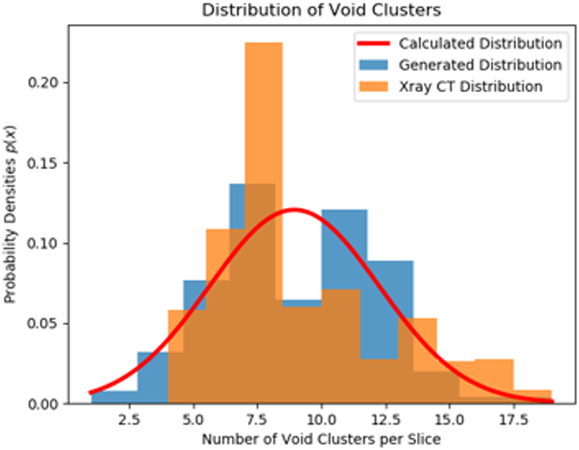 gathered in Quantification of Resin and Void Clusters.

In Figure 17, the orange histogram shows the distribution obtained directly from the x-ray CT data, the red curve shows the calculated PDF of this data, and the blue histogram shows a randomly generated distribution obtained by sampling the red PDF. It should, of course, be noted that probability is at play in the sampling of the red curve; the blue distribution will change with each realization of the microstructure. Meanwhile, the red and orange distributions come directly from the x-ray CT data and therefore are fixed.

Synthetic generation procedure

Figure 18 shows a procedure for constructing a synthetic microstructure from the PDFs. A uniform rectangular cross-section for the slice is first created, Figure 18(a). In Figure 18(b), the surface undulation obtained from the microstructure characterization (Supplementary Material Appendix B.4) is applied to the top and bottom of the slice. Next, utilizing the previously generated PDFs, isolated voids and void clusters are introduced into the domain, Figure 18(c) and (d), respectively. The increase in the void fraction that occurs after introducing the void clusters is accounted for by converting a portion of the seeded voids back into material,Figure 18(e). The void/void cluster configuration is finalized as shown in Figure 18(f). In a similar manner, isolated resin material points (Figure 18(g)) and resin clusters are introduced (Figure 18(h)) into the slice. The fully reconstructed slice is then obtained by matching the resin volume fraction as shown in Figure 18(i). Additional details on the implementation of resin and void clusters are provided in Supplementary Material Appendix D.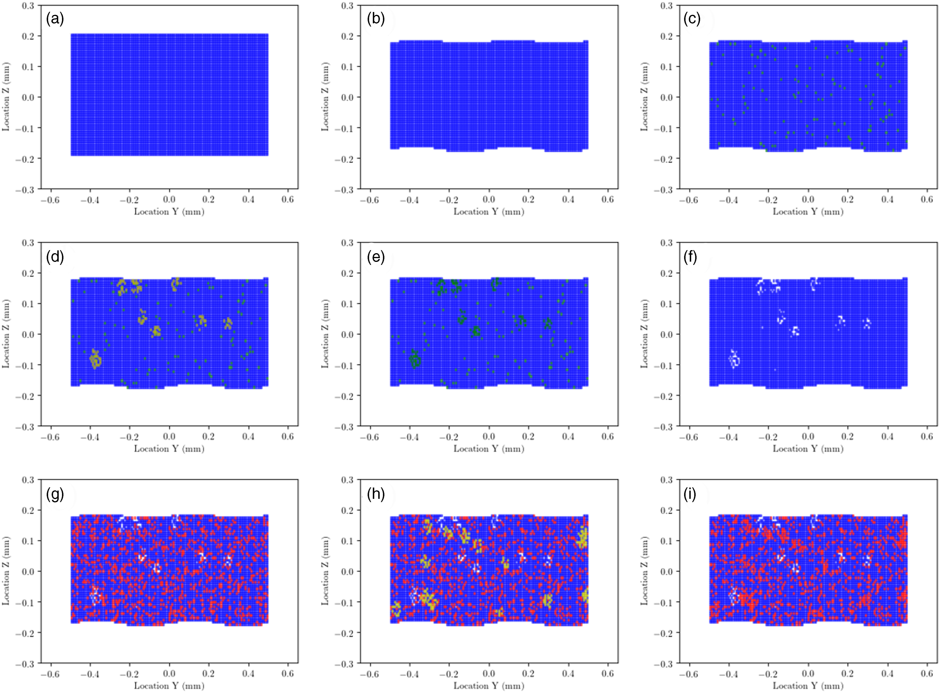

Qualitatively, the reconstructed slice and the experimentally observed slice share many common features. Quantification of the differences between the actual CT slice and the reconstructed slice is underway. The accurate synthetic reconstruction of the microstructure will be used for further computational exploration. Ultimately, by observing the effect of changing the PDF on the predicted mechanical properties, one can optimize the microstructure and explore how particular structural features affect the mechanical behavior.

Four distinct reconstructions

Four distinct realizations of the microstructure were generated and simulated. Figure 19 shows a comparison of the PDFs for each realization. Each row of the image is a different realization labeled R1 to R4. As mentioned previously, each realization has a different histogram of statistics (blue) that matches the PDF in (red). The first column shows the distribution of void clusters on each slice. The number of void clusters ranges from 2.5 to 17.5 on each slice. The second column shows the distribution of resin clusters on each slice. There are many more resin clusters than void clusters on each slice. This distribution ranges from 20 to approximately 40 void clusters. The final two columns show the distribution in void fraction and the distribution in resin volume fraction, respectively.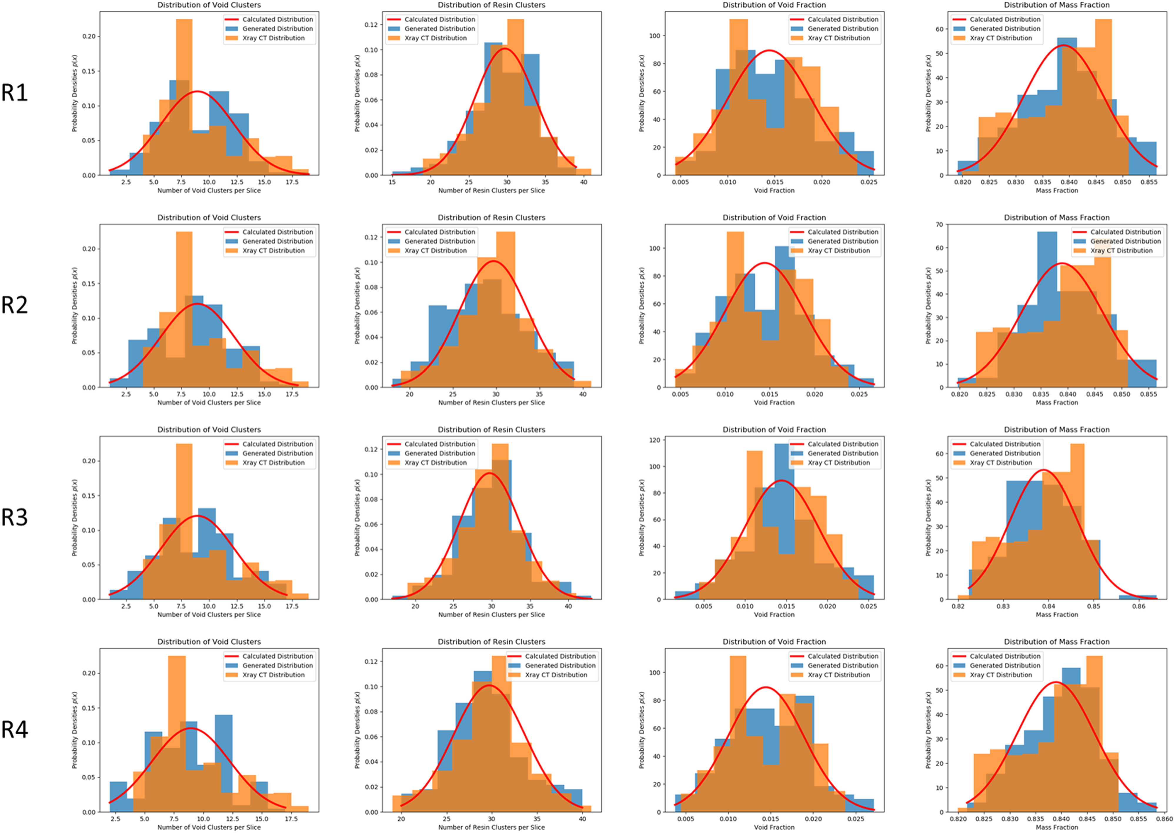

Following the PD simulation approach of the previous section, the stress–strain response of each realization was simulated. Figure 20 shows the resulting damage contours at a failure strain between 2.0% and 2.2%. The damage contours show both similarities and differences with the x-ray CT damage contours. Unlike the x-ray CT generated cells, damage occurs more towards the middle of the specimen as opposed to the boundaries. Additionally, there is less damage on the surface of the cell than found in the x-ray CT cell. However, similar to the x-ray CT generated specimen, longitudinal damage is observed.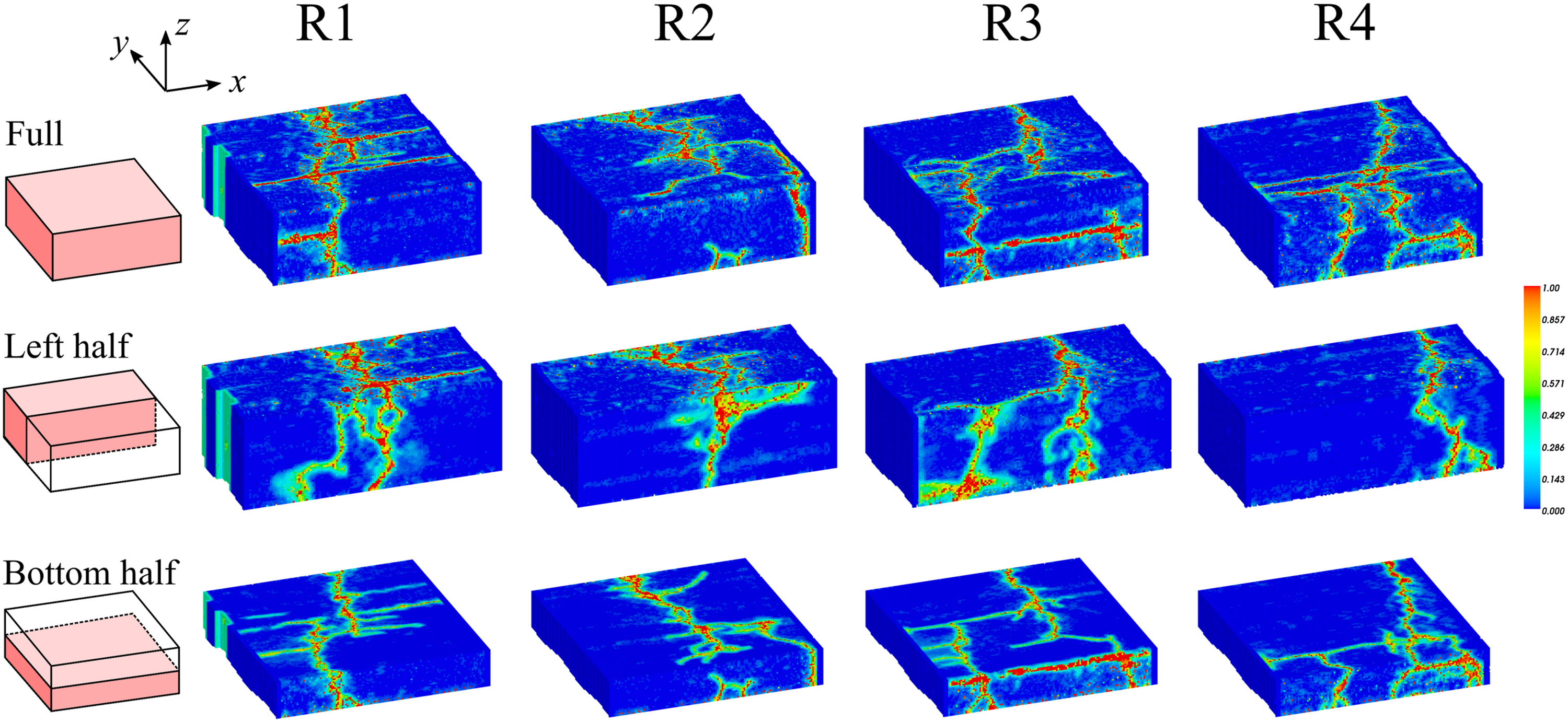

Figure 21 shows that the stress–strain responses for each realization are very consistent with one another and match the experimental curve very well. The bulk stress–strain response is yarn-dominated even though microstructural differences lead to different damage morphologies as observed in Figure 20.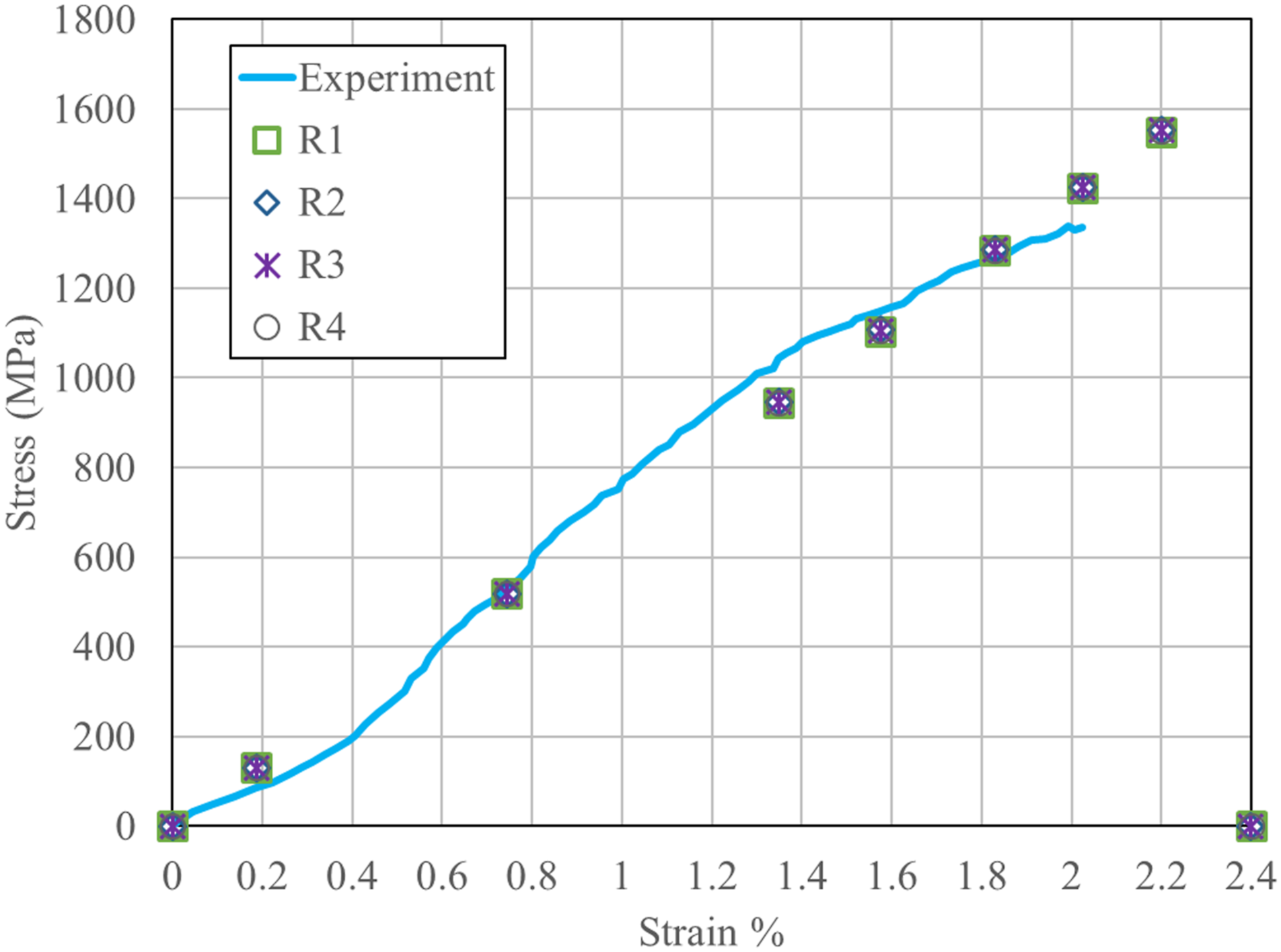

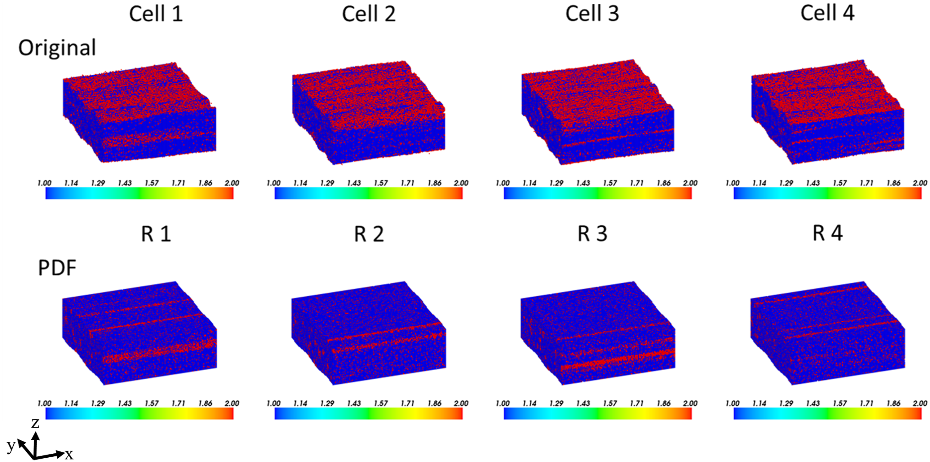
Finally, Figure 22 compares the damage initiation in a model of the x-ray CT structure and in the synthetic realization 2. Similar failure characteristics are observed in the initial snapshots (columns 1 and 2). Major differences in the failure behavior begin at column 3. At this snapshot, in cell 1, the damage continues to propagate transversely to the edge of the specimen. In R2, however, the damage initiates in the middle of the specimen. In columns 4–7 of both representations, damage propagates in the longitudinal direction. The differences in failure behavior can potentially be explained by the difference in the material association between the x-ray CT structure and the synthetic realization as shown in Figure 23. Specifically, there is a resin-rich layer at the top surface of the experimental composite which is not captured in the PDF generated synthetic realization. The influence of this resin layer on failure behavior will be explored in future work.

Co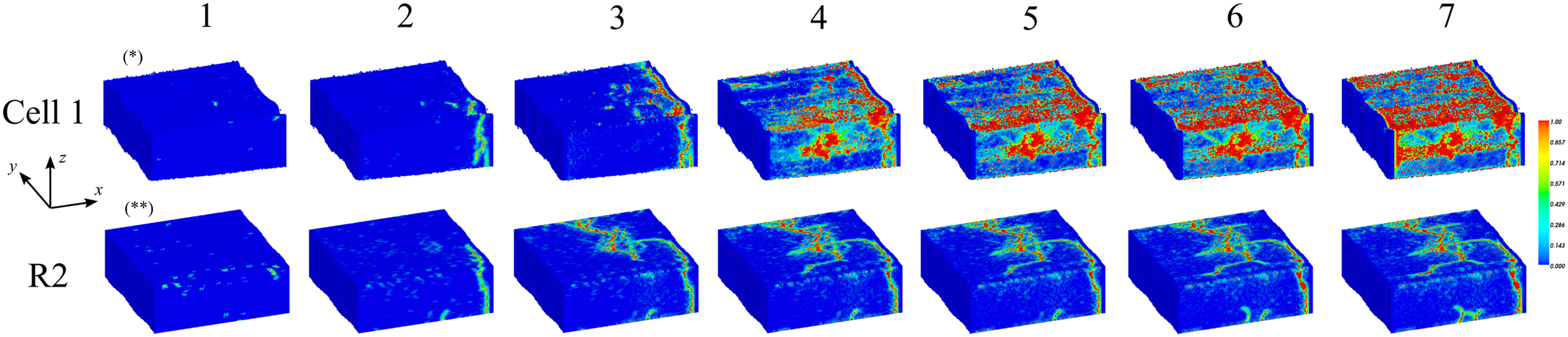nclusions and future work

This work describes the development of a method for accurately predicting the deformation and failure of CNT yarn/polymer composites using the peridynamic theory. The heterogeneity of the microstructure and the resulting anisotropic behavior were accommodated within the peridynamic framework by using different bond types for CNT yarn and polymer resin. Additionally, an off-axis modulus function following a Gaussian variation has been utilized to account for CNT bundles that are not aligned with the major yarn direction. A number of peridynamic models were generated using new techniques for processing x-ray CT reconstructions. During the process, special care was taken to maintain consistency between the experimental specimen and the peridynamic models in terms of their fiber and matrix volume ratios, void fraction, and surface undulation.

Characterization of the x-ray CT data was extended by constructing probability density functions for yarn, resin, and void materials for each slice. Further, the DBSCAN algorithm was employed to detect shape, size, and quantity of resin and void clusters in each slice. This additional characterization effort provided information needed to generate synthetic peridynamic models that share the characteristics of the x-ray CT-based models, qualitatively and quantitatively. Simulations of the tension test of CNT yarn/polymer composites were performed using the generated peridynamic models.

The following conclusions are drawn:

• X-ray CT-based heterogenous peridynamic model simulations capture the experimentally observed stress-strain response as well as the failure strain with good agreement.

• Results reveal that the damage is most prevalent on the exposed surfaces and primarily aligned with the yarn direction, which is consistent with the experiment.

• Sharp gradients on the surface provide preferential sites for failure initiation.

• Clusters of resin and voids facilitate failure propagation.

• Synthetically generated heterogenous peridynamic model simulations also capture the stress–strain response. The failure morphology shows damage aligned with the yarn direction.

• Compared to the X-ray CT-based model results, fracture initiation in synthetic models typically occurs near the midspan as opposed to multiple locations.

• The surface damage in synthetic models is not as pronounced as that seen in the x-ray CT-based models.

There are three main differences between the x-ray CT-based and synthetically generated peridynamic models: (1) the x-ray CT-based model, and thus the actual specimen, has a higher concentration of resin at the exposed surfaces, (2) the continuity of void and resin clusters along the yarn direction, and (3) the surface undulations of the synthetically generated models have smoother variation and they do not vary with each slice, thus reducing the chances of initiating cracks from the surfaces. These differences lead to the discrepancy between the failure morphologies predicted by the two types of peridynamic models. Although the specimen level stress-strain response and failure strain are both predicted with good agreement, in order to effectively utilize the synthetic models for exploration of the design space to maximize stiffness and strength, the synthetic models need to closely represent the actual microstructural characteristics. This work is the subject of a separate ongoing study. Once complete, the influences of void fraction, void clusters, shape and size of resin clusters, and resin distribution through the thickness of the composite on the mechanical behavior of the CNT yarn/polymer composites will be explored.

Supplemental Material

sj-pdf-1-jcm-10.1177_00219983211065718 – Supplemental Material for Microstructural exploration of a carbon nanotube yarn reinforced composite using a peridynamic approach

Supplemental Material, sj-pdf-1-jcm-10.1177_00219983211065718 for Microstructural exploration of a carbon nanotube yarn reinforced composite using a peridynamic approach by Forrest Baber, Jae-Woo Kim, Godfrey Sauti, Russell A Wincheski, Benjamin D Jensen, Kristopher E Wise, Emilie J Siochi and Ibrahim Guven in Journal of Composite Materials

Footnotes

Acknowledgments

The authors gratefully acknowledge the partial support provided by the National Aeronautics and Space Administration (NASA) through The Institute for Ultra-Strong Composites by Computational Design (US-COMP), a NASA Space Technologies Research Institute (STRI).

Declaration of conflicting interests

The author(s) declared no potential conflicts of interest with respect to the research, authorship, and/or publication of this article.

Funding

The author(s) disclosed receipt of the following financial support for the research, authorship, and/or publication of this article: This study is supported by University of Utah (10044107).

ORCID iD

Ibrahim Guven

Supplemental Material

Supplemental material for this article is available online.

References

Monthioux

Kuznetsov

. Who should be given the credit for the discovery of carbon nanotubes? Carbon 2006; 44(9): 1621–1623.

Treacy

MMJ

Ebbesen

Gibson

. Exceptionally high Young’s modulus observed for individual carbon nanotubes. Nature 1996; 381(6584): 678–680.

Wong

Sheehan

Lieber

. Nanobeam mechanics: elasticity, strength, and toughness of nanorods and nanotubes. Science 1997; 277(5334): 1971–1975.

Ruoff

Qian

Liu

. Mechanical properties of carbon nanotubes: theoretical predictions and experimental measurements. C R Phys 2003; 4(9): 993–1008.

Lourie

Dyer

, et al. Strength and breaking mechanism of multiwalled carbon nanotubes under tensile load. Science 2000; 287(5453): 637–640.

Kim

Sauti

Cano

, et al. Assessment of carbon nanotube yarns as reinforcement for composite overwrapped pressure vessels. Compos Part A Appl Sci 2016; 84: 256–265.

Silling

. Reformulation of elasticity theory for discontinuities and long-range forces. J Mech Phys Solids 2000; 48(1): 175–209.

Kilic

Agwai

Madenci

. Peridynamic theory for progressive damage prediction in center-cracked composite laminates. Compos Struct 2009; 90(2): 141–151.

Bobaru

Doh Ha

. Damage progression from impact in layered glass modeled with peridynamics. Cent Eur J Eng 2012; 2(4): 551–561.

10.

Bobaru

. Studies of dynamic crack propagation and crack branching with peridynamics. Int J Fract 2010; 162(1): 229–244.

11.

De Meo

Zhu

Oterkus

. Peridynamic modeling of granular fracture in polycrystalline materials. J Eng Mater Technol 2016; 138(4): 041008.

12.

Madenci

Oterkus

. Peridynamic theory and its applications. Berlin, Germany: Springer, 2014, pp. 19–43.

13.

Oterkus

Madenci

. Peridynamic analysis of fiber-reinforced composite materials. J Mech Mater Struct 2012; 7(1): 45–84.

14.

Askari

Silling

. Peridynamic analysis of damage and failure in composites. In: 44th AIAA aerospace sciences meeting and exhibit, Reno, Nevada, 9–12 January 2006, p. 88.

15.

Colavito

. Peridynamics for failure and residual strength prediction of fiber-reinforced composites. PhD Thesis, Tucson, AZ: The University of Arizona, 2013.

16.

Bobaru

Silling

. Peridynamic 3D models of nanofiber networks and carbon nanotube‐reinforced composites. In: Proceedings of the 8th International Conference on Numerical Methods in Industrial Forming Processes, Columbus, OH, 13–17 June 2004, pp. 1565–1570.

17.

Rahman

Foster

. Bridging the length scales through nonlocal hierarchical multiscale modeling scheme. Comput Mater Sci 2014; 92: 401–415.

18.

Decklever

Spanos

. Nanocomposite material properties estimation and fracture analysis via peridynamics and Monte Carlo simulation. Probabilistic Eng Mech 2016; 44: 77–88.

19.

Kim

Sauti

Wincheski

, et al. Unidirectional carbon nanotube yarn/polymer composites. NASA/TM 2018 Jul 1: 220081.

20.

Schneider

Rasband

Eliceiri

. NIH Image to ImageJ: 25 years of image analysis. Nat Methods 2012; 9(7): 671–675.

21.

Sertse

Goodsell

Ritchey

, et al. Challenge problems for the benchmarking of micromechanics analysis: level I initial results. J Compos Mater 2018; 52(1): 61–80.

22.

Madenci

Yaghoobi

Barut

, et al. Peridynamic unit cell for effective properties of complex microstructures with and without defects. Theor Appl Fract Mech 2020; 110: 102835.

23.

Pedregosa

Varoquaux

Gramfort

, et al. Scikit-learn: machine learning in Python. J Mach Learn Res 2011; 12: 2825–2830.

24.

Ester

Kriegel

Sander

, et al. A density-based algorithm for discovering clusters in large spatial databases with noise. In: KDD Conference, Portland, OR, 2 August 1996, Vol. 96(34), pp. 226–231.

25.

Silling

Epton

Weckner

, et al. Peridynamic states and constitutive modeling. J Elast 2007; 88(2): 151–184.

26.

Gerstle

. Introduction to practical peridynamics: computational solid mechanics without stress and strain. Singapore: World Scientific Publishing Company, 2015.

27.

Trageser

Seleson

. Bond-based peridynamics: a tale of two Poisson’s ratios. J Peridyn Nonlocal Model 2020; 2(3): 278–288.

28.

Ganesan

Muthusamy

. Mechanical properties of high temperature cyanate ester/BMI blend composites. Polym Compos 2009; 30(6): 782–790.

29.

Voss

Fabian

Feucht

, et al. Performance evaluation of cyanate ester resin. In: 20th IEEE/NPSS Symposium on Fusion Engineering, San Diego, CA, 14 Oct 2003, pp. 181–184. IEEE.

30.

Hamerton

Hay

. Recent technological developments in cyanate ester resins. High Perform Polym 1998; 10(2): 163–174.

31.

Ganguli

Dean

Jordan

, et al. Mechanical properties of intercalated cyanate ester-layered silicate nanocomposites. Polymer 2003; 44(4): 1315–1319.

32.

Yang

Greenfeld

Wagner

. Toughness of carbon nanotubes conforms to classic fracture mechanics. Sci Adv 2016; 2(2): e1500969.

33.

Takakura

Beppu

Nishihara

, et al. Strength of carbon nanotubes depends on their chemical structures. Nat Commun 2019; 10(1): 3040–3047.

Supplementary Material

Please find the following supplemental material available below.

For Open Access articles published under a Creative Commons License, all supplemental material carries the same license as the article it is associated with.

For non-Open Access articles published, all supplemental material carries a non-exclusive license, and permission requests for re-use of supplemental material or any part of supplemental material shall be sent directly to the copyright owner as specified in the copyright notice associated with the article.

0.00 MB

2.06 MB