Comparative study on the evolution of process-induced residual stresses and deformations in thick and ultra-thick vacuum-infused laminates for wind turbine blades

Abstract

The current research provides a thorough numerical investigation to shed light on the evolution of longitudinal and interlaminar normal residual stresses and induced deformations in thick and ultra-thick vacuum-infused laminates. The impact of resin curing during the mold-filling stage on residual stresses is also examined through a non-isothermal simulation of the mold filling with reactive resin for both thick and ultra-thick laminates. In addition, the effect of two resin-mixing types, both online and offline, is studied on the residual stresses and induced deformations. An in-house code namely VIsim is employed to conduct numerical simulations for the laminates, which involve non-isothermal mold filling with reactive resin, flushing, bleeding, and thermo-chemo-mechanical analysis during the curing stage. The study analyzes two E-glass/epoxy laminates with thicknesses of 50 mm and 100 mm each with a length of 1m. The results indicate that the distribution of longitudinal residual stresses in the thickness direction differs significantly between thick and ultra-thick laminates. However, the maximum interlaminar normal stress for the ultra-thick laminate is 143% greater than that of the thick laminate at the end of the process. The influence of resin mixing type is also found to be more significant on the residual stresses of ultra-thick laminates than thick laminates. Additionally, considering resin curing during the initial three stages of the Vacuum Infusion (VI) process through non-isothermal numerical simulation significantly affects the deformation of both thick and ultra-thick laminates.

Keywords

cure behavior residual/internal stress thick laminates resin mixing types non-isothermal mold filling

Introduction

The growing demand for much longer and more reliable wind turbine blades highlights the need to improve the quality of laminates produced using the Vacuum Infusion (VI) process, a widely employed technique in the wind industry. In wind turbine blades, the primary structural element responsible for handling bending loads is the main girder. The laminate thickness for this part typically measures around 50 mm, while the root section connecting the blade to the hub can reach a thickness of up to 100 mm.¹ Consequently, thick and ultra-thick section laminates are crucial components in wind turbine blade structures. However, incorporating these laminates poses distinctive challenges during the manufacturing process. The development of residual stresses within these laminates during the manufacturing process can significantly impact their performance. These stresses may lead to various defects, including matrix cracking, delamination,^2,3 warpage,⁴ and reduced fatigue life of the laminate.⁵ A first step in mitigating process-induced residual stresses and deformations is developing a thorough understanding of the underlying physics, mechanisms, and the impact of each stage of the VI process and its parameters on residual stress evolution.

The VI process generally comprises four stages: two major stages (mold filling with resin and curing) and two minor stages (flushing and bleeding). During the flushing stage, the resin is continuously injected after the mold has been filled, while the bleeding stage consists of removing excess resin from the mold.

The curing stage is crucial for processing thick-section composites due to the combination of low thermal conductivity and exothermic reaction of thermoset resins. During this stage, the laminate may encounter local high temperatures, significant thermal gradients, and a substantial degree of cure (DoC) gradients. While the manufacturer’s recommended cure cycle (MRCC) is suitable for curing thin-section laminates, it may be inadequate for addressing the requirements of thick-section laminates.⁶ Residual stress in a laminate arises from a mismatch in the properties of composite constituents and adjacent plies, as well as temperature and DoC gradients that develop within the laminate during the curing process. These gradients become more pronounced as the laminate thickness increases.⁷ Moreover, tool-part interactions significantly influence composite laminate deformation during processing,⁸ particularly for thin laminates.⁹

In a study by Lahuerta et al.,¹⁰ it was found that for an E-Glass/Epoxy laminate with a thickness of 65 mm, the variations in mechanical properties along the thickness direction could be attributed to the temperature variations experienced during the curing stage. Moreover, Zhou et al.¹¹ have demonstrated that the mechanical properties of thick-section laminates can be significantly influenced by the stress distribution history during the curing stage. Therefore, the performance of thick-section composites is significantly impacted by their processing history.⁷ Hu et al.¹² conducted a numerical and experimental study to investigate the impact of non-uniform gelation on residual stress in a 10 mm thick CFRP laminate composed of 80 stacks of T300/DL1803 unidirectional prepregs.

Apart from the curing stage, the residual stress evolution in thick-section laminates can also be influenced by the initial three stages of the VI process, which include mold filling, flushing, and bleeding. The significant duration of the mold-filling stage in the VI process for thick-section laminates allows the resin substantial time to progress in the curing process. Therefore, resin curing during the three initial stages of the VI process should be considered.

Two approaches can be employed for the above-mentioned purpose. The conventional method involves assuming uniform DoC and temperature fields with predetermined magnitudes prescribed throughout the laminate at the onset of the curing stage. The magnitude of the uniform DoC field is calculated using the curing kinetic equation of the infused resin at ambient temperature, considering the time elapsed until the bleeding stage is completed. The temperature field magnitude is also assumed to be equivalent to the ambient temperature. Consequently, this approach eliminates the need to simulate the initial three stages of the VI process. Many researchers have employed this approach to optimize the curing stage of thick-section laminates.^1,13–15 This approach ignores the non-uniform nature of the DoC and temperature fields, as well as the increase in temperature and DoC due to the resin’s exothermic reaction during curing in the initial three stages of the VI process. Although this approach proves useful for thin-section laminates, its applicability becomes questionable when dealing with thick-section laminates. For thick-section laminates, it is shown that the non-uniform temperature and DoC field distributions at the end of the mold-filling stage can result in varying curing histories for different laminate locations.¹⁶ The second approach involves direct numerical simulation of all stages of the VI process, encompassing mold filling, flushing, bleeding, and curing.¹⁷ A non-isothermal mold-filling simulation utilizing reactive resin should be employed to account for resin curing during the mold-filling stage. This type of numerical simulation is necessary for accurately capturing the intricate interplay between the chemical and thermal properties of the resin and the filling pattern of the mold. Researchers have employed various commercial software packages, such as PAM-RTM,^16,18,19 STAR-CCM+,²⁰ ANSYS FLUENT,²¹ and others, as well as in-house codes,^17,22–24 to simulate non-isothermal mold filling in VI or RTM processes. In some cases, the analysis of residual stresses involves coupling ABAQUS software with the simulation software used for the mold-filling stage.²⁰

To investigate the influence of resin curing during mold filling on process-induced residual stress within laminates, Nasiri and Abedian¹⁷ developed a two-dimensional code (VIsim) capable of simulating all stages of the VI process. Additional details on the VIsim code, its underlying algorithm, and validation test cases can be found in their work. They also studied the impact of resin curing during the initial three stages of the VI process on process-induced residual stress at the end of the curing stage for an ultra-thick laminate.

It is crucial to note that for a comprehensive understanding of process-induced residual stresses within laminates, examining the magnitudes of residual stresses at the end of the curing stage is insufficient. A thorough investigation of residual stress evolution during the curing stage, along with an explanation of the underlying mechanisms contributing to residual stress formation, is necessary. Additionally, the thickness of the laminate and the resin mixing type can influence residual stress evolution within laminates. To the best of the authors’ knowledge, this gap in the literature has not been addressed. The present study aims to fill this gap by providing a comprehensive analysis of residual stress evolution and deformation in thick and ultra-thick laminates, considering the effects of the initial three stages of the VI process.

The current research offers a thorough numerical investigation that aims to shed light on the development of longitudinal and interlaminar residual stresses, along with the relevant deformations, in thick and ultra-thick E-Glass/Epoxy laminates. The underlying mechanisms responsible for residual stress formation are discussed to provide a better understanding of the development and evolution of these stresses. The study examines the impact of resin curing during the initial three stages of the VI process on residual stress development within the laminates. This goal is accomplished through a comparative analysis of the outcomes obtained by employing the two previously mentioned approaches. The resin system components can either be mixed before the mold-filling stage, referred to as offline mixed resin, or combined during the mold-filling stage itself, known as online mixed resin. The impact of resin mixing methods on temperature and DoC distributions at the end of the bleeding stage, as well as their influence on residual stress development within the laminates, is investigated. The study focuses on examining two E-Glass/Epoxy laminates with a length of 1m and thicknesses of 50 mm and 100 mm, respectively. The VIsim code¹⁷ is employed to conduct numerical simulations for the laminates, which involve non-isothermal mold filling with reactive resin, flushing, bleeding, and thermo-chemo-mechanical analysis during the curing stage. It should be noted that this simulation framework does not account for bubble formation or void migration during mold filling, as the primary objective is to study the curing behavior of laminates by considering the resin curing during the mold-filling stage. Therefore, while the model provides reliable predictions of resin flow and cure behavior, it cannot estimate the final void content within the laminates.

Material constitutive models

In the current numerical study, Metyx biaxial E-glass fabrics with a superficial density of 850 g/m², and the two-component Airstone^TM 780 E epoxy resin and 785 H hardener system are employed as fibrous reinforcement and resin system, respectively. The resin and E-Glass fiber densities ( $ρ_{r}$ , $ρ_{f}$ ) are 1105 kg/m³ and 2600 kg/m³, respectively.¹ This section outlines several important material constitutive models required to simulate all stages of the VI process for different numerical scenarios. Additional material models not covered here can be found in Ref. 17.

Permeability and compaction behavior of the reinforcement

The longitudinal ( $S_{l}$ ) and out-of-plane ( $S_{t}$ ) permeability, as well as the unloading behavior (wet) models for the fabric, are presented in equation (1),²⁵ 2, and 3,²⁵ respectively:

S_{l} = 2.16 \times 10^{- 8} e^{- 9.93 V_{f}}

(1)

S_{t} = (1.38 e^{- 3.39 V_{f}} + 0.1) \times 10^{- 11}

(2)

V_{f} = 0.2531 {P_{c}}^{0.0524}

(3)

where

V_{f}

and

P_{c}

denote fiber volume fraction and compaction pressure of the fabric, respectively. Equation (2) is derived by combining insights from the out-of-plane permeability behavior of a biaxial carbon fabric, as reported in Ref. 26, and the permeability range observed for a biaxial E-glass fabric, as noted in Ref. 27. The compaction pressure is calculated by subtracting the resin pressure from the atmospheric pressure, assumed to be 100 kPa in this study. The permeability model for the flow mesh (Green Flow 75) with a thickness of 0.75 mm is given by equation (4):²⁶

S_{l}^{f l o w m e s h} = (9.4 - 1.69 \ln (P_{c})) \times 10^{- 9}

(4)

where

S_{l}^{f l o w m e s h}

represents the permeability of the flow mesh in the longitudinal direction.

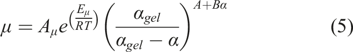
Rheology model

The resin viscosity model, which accounts for the influence of both DoC and temperature, can be represented by the following equation²⁸:

μ = A_{μ} e^{(\frac{E_{μ}}{R T})} {(\frac{α_{g e l}}{α_{g e l} - α})}^{A + B α}

(5)

where

A_{μ}

E_{μ}

A

, and

B

are constants, as presented in Table 1.

α_{g e l}

represents the DoC at the gel point, which is equal to 0.69 for the Airstone resin system.²⁸

Table 1.

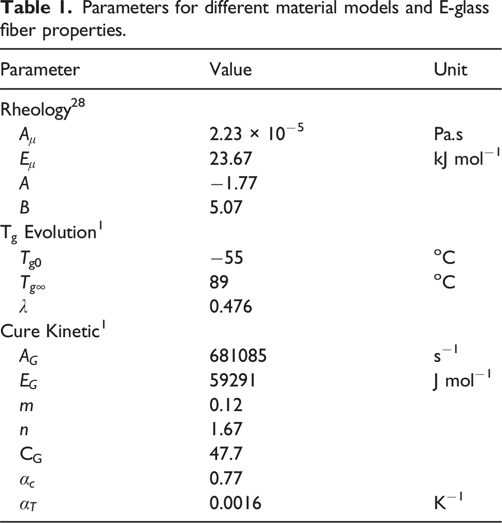
Parameters for different material models and E-glass fiber properties.

Parameter	Value	Unit
Rheology²⁸
$A_{μ}$	2.23 × 10⁻⁵	Pa.s
$E_{μ}$	23.67	kJ mol⁻¹
A	−1.77
$B$	5.07
$T_{g}$ Evolution¹
T_g0	−55	^oC
$T_{g \infty}$	89	^oC
$λ$	0.476
Cure Kinetic¹
$A_{G}$	681085	s⁻¹
$E_{G}$	59291	J mol⁻¹
$m$	0.12
$n$	1.67
$C_{G}$	47.7
$α_{c}$	0.77
$α_{T}$	0.0016	K⁻¹

Thermal and chemical models

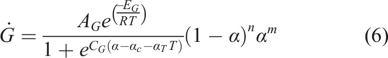
The cure kinetic model of the resin system can be described by¹:

\dot{G} = \frac{A_{G} e^{(\frac{- E_{G}}{R T})}}{1 + e^{C_{G} (α - α_{c} - α_{T} T)}} {(1 - α)}^{n} α^{m}

(6)

where

α

represents the DoC.

α_{c}

and

α_{T}

are coefficients that adjust the transition of the cure kinetic from chemical to diffusion control.

A_{G}

C_{G}

E_{G}

, m, and n are constants of the model, which are presented in Table 1. The total heat of the reaction per unit mass (

H_{R}

) is equal to 434 J/g for the Airstone resin system.¹

The evolution of the glass transition temperature (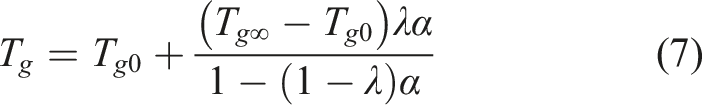 $T_{g}$ ) as a function of resin conversion is modeled using the Di-Benedetto equation²⁹;

T_{g} = T_{g 0} + \frac{(T_{g \infty} - T_{g 0}) λ α}{1 - (1 - λ) α}

(7)

where

T_{g 0}

and

T_{g \infty}

are glass transition temperatures of the resin at uncured and fully cured states, respectively.

λ

is the model constant. The parameters of this model are also presented in Table 1.

The total volumetric shrinkage of the Airstone resin system is 5.6%.³⁰ Therefore, according to the relationship between volumetric and linear shrinkages,³¹ the corresponding linear shrinkage of the resin would be 1.83%. The linear shrinkage of the resin ( $γ_{r}$ ) as a function of the DoC has been modeled using a linear function as follows³⁰:

γ_{r} = γ_{α} α

(8)

where

γ_{α}

is the maximum linear shrinkage of the resin.

Six scenarios for numerical investigation

Six distinct numerical simulation scenarios are designed to explore the issues mentioned at the end of Section ‘Introduction'. Table 2 describes the six scenarios employed for the numerical simulation of the VI process in this study. In the first three scenarios, the 50 mm thickness laminate is considered, while for the remaining scenarios, the laminate thickness is assumed to be 100 mm. The online resin mixing method is utilized for the first and fourth scenarios, whereas the offline resin mixing approach is employed for the second and fifth scenarios. All stages of the VI process, including mold filling, flushing, bleeding, and curing, are numerically simulated using VIsim for the first, second, fourth, and fifth scenarios. On the other hand, only the curing stage of the VI process is numerically simulated for the third and sixth scenarios. In these two scenarios, the impact of mold filling, flushing, and bleeding stages on the resin conversion field is accounted for by considering a uniform resin conversion field at the beginning of the curing stage. The magnitude of this uniform resin conversion field is determined by employing the resin’s cure kinetic equation (Equation (6)) at ambient temperature and the time elapsed until the end of the bleeding stage. Additionally, at the onset of the curing stage for these scenarios, the temperature field within the laminate is assumed to be uniform and at ambient temperature (25°C).

Table 2.

Description of different scenarios for numerical investigation.

Scenario	Laminate Thickness (mm)	Resin-mixing type	Initial resin conversion field for curing stage	Initial temperature field for curing stage
1	50	Online	End of bleeding	End of bleeding
2	50	Offline	End of bleeding	End of bleeding
3	50	-	Uniform (Equation (6))	Ambient temperature
4	100	Online	End of bleeding	End of bleeding
5	100	Offline	End of bleeding	End of bleeding
6	100	-	Uniform (Equation (6))	Ambient temperature

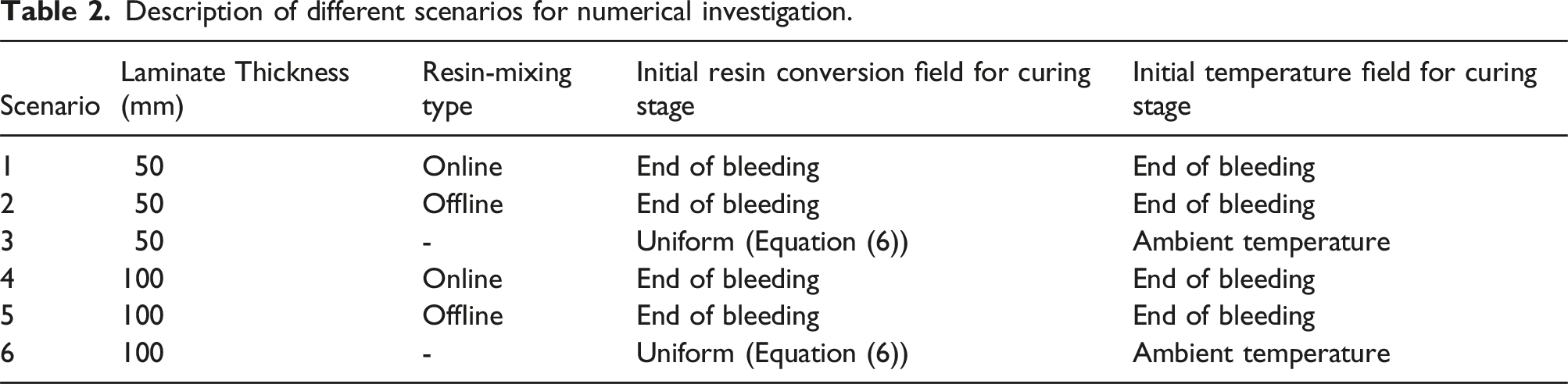
The distinction between online and offline resin mixing lies in the DoC of the resin at the inlet points. For online mixing, the DoC is set to 0.001 during the mold filling and flushing stages, indicating immediate resin mixing before mold entry, while the inlet temperature is maintained at 25°C. In contrast, for offline mixing, the DoC at the inlet points evolves during the above-mentioned stages according to the resin cure kinetic equation (Equation (6)) and the elapsed time from the beginning of the process. Note that the temperature is kept constant (25°C) at the inlet points for both mixing methods during these stages.

The numerical investigation is performed on two E-glass/epoxy laminates with identical lengths of 1 m and thicknesses of 50 mm and 100 mm. A flow mesh of 714 mm and 857 mm in length is placed over the 100 mm and 50 mm thick laminates, respectively. The chosen flow mesh lengths ensure that no dry regions form because of the lead-lag effect of the flow front. The laminates are modeled in two dimensions, assuming no temperature and resin conversion gradients in the width direction. Furthermore, the plane strain assumption is employed for the thermo-chemo-mechanical analysis.

Figure 1 illustrates the inlet and outlet locations, thermal and mechanical boundary conditions, five designated sensing points (SPs, labeled a-e), and two Longitudinal and Transversal Data collection Lines (LDLine and TDLine) for the model with a thickness of 100 mm. It is important to note that for the model with a thickness of 50 mm, all specified parameters and conditions are identical, except for the flow mesh length.

Figure 1.

Details of the laminate model and its boundary conditions (100 mm thickness).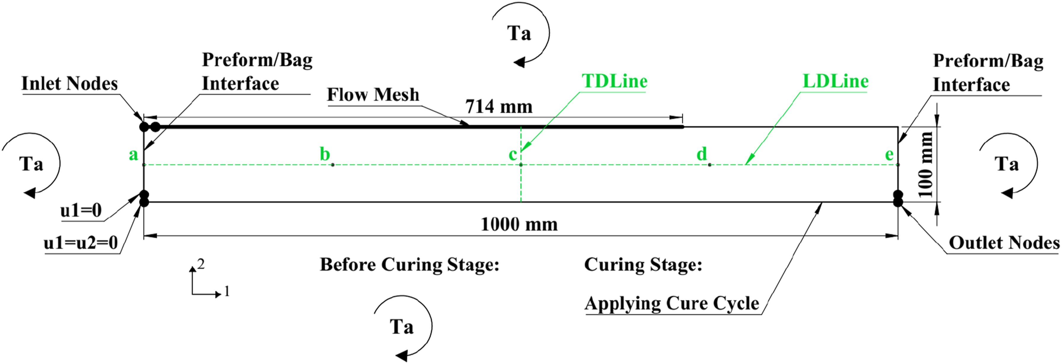

Both models with 50 mm and 100 mm thicknesses are discretized using 100 and 16 rectangular elements in the longitudinal and transverse directions, respectively. In the transverse direction, a uniform element size is maintained, whereas smaller elements are employed near the edges in the longitudinal direction to ensure an accurate representation of the interlaminar normal stress distribution. Initially, the model was discretized along the longitudinal direction with 70 elements. To enhance the resolution near the edges, the first five elements from each edge were subdivided into three elements each, while the next five elements were further subdivided into two elements each. Consequently, the final discretization of the model along the longitudinal direction resulted in a total of 100 elements.

As mentioned at the beginning of Section ‘Material constitutive models', Metyx biaxial E-glass fabrics with a superficial density of 850 g/m2 and the two-component Airstone^TM 780E epoxy resin and 785H hardener system are employed as fibrous reinforcement and resin system, respectively. Therefore, all material constitutive models described in this section and in Ref. 17 are used in the numerical simulations of the thick and ultra-thick laminates. The porosity of the flow mesh is considered to be 0.7 in the current study. Moreover, a region with permeability of 1e-10 m² is considered at the two ends of the laminate to enhance permeability in these locations. This region is considered based on the experimental observation that out-of-plane permeability at the vacuum bag/laminate interface is higher than that within the laminate.²⁶ Since the thicknesses of the laminates (50 mm and 100 mm) are comparatively high, the thickness of this region is considered to be 2 mm.

In the laminates with thicknesses of 50 mm and 100 mm, the number of layers of biaxial E-glass fabrics is approximately 80 and 160, respectively. Therefore, in the thermos-chemo-mechanical analysis, instead of modeling 0 and 90-degree plies separately, the entire laminate is assumed to be an orthotropic material. The stiffness matrix of the equivalent orthotropic material is computed by applying the stiffness averaging method³² to the stiffness matrices of the 0 and 90-degree plies.

During the mold-filling stage, the inlet and outlet pressures are maintained at 100 kPa and 0 kPa, respectively. Once the mold is filled, the resin infusion process continues for an additional 5 minutes with the same inlet and outlet pressures as the mold filling stage, referred to as the flushing stage. Subsequently, the resin inlet is closed, and excess resin is removed through the outlet for 5 minutes at an outlet pressure of 0 kPa, known as the bleeding stage. Following the bleeding stage, the curing stage begins by applying the manufacturer’s recommended cure cycle³⁰ to the bottom of the laminate. To allow the laminate to reach thermal equilibrium with ambient temperature, an additional holding phase is incorporated at the end of the cooling phase of the MRCC. As a result, the cure cycle consists of the following stages: a heating phase that increases the temperature from 25°C to 70°C at a rate of 0.3°C/min, a holding phase that maintains the temperature at 70°C for 4 hours, a cooling phase that decreases the temperature from 70°C to 25°C at a rate of 0.5°C/min, and a final holding phase that maintains the temperature at 25°C for 3 hours.

In the current research, the mechanical behavior of materials is modeled using the Cure Hardening Instantaneously Linear Elastic (CHILE) model, as outlined in Ref. 17. In this approach, the modulus development during curing is assumed to be elastic, with a constant modulus at each time step that only varies with temperature and DoC. Given the simple cure cycle and ascending modulus development (with no devitrification during curing), this assumption is deemed valid based on Ref. 33.

The cure cycle and selected times (STs) for presenting simulation results are illustrated in Figure 2. The selected time points chosen for the result presentation are 100min (ST1), 150min (ST2), 270min (ST3), 390min (ST4), 480min (ST5) and 660min (ST6). The selected times (STs) were carefully chosen to capture the critical evolution of key parameters during the curing process. Selected times (ST2, ST4, ST5, and ST6) were chosen at the end of each curing phase to systematically evaluate phase-dependent effects on the evolution of DoC, temperature, resin modulus, and residual stress within the laminates. To monitor the significant parameter variations occurring during the 70°C holding phase, a time point (ST3) was placed at the midpoint of this phase. To capture the accelerated curing observed in ultra-thick laminates compared to thick laminates, an additional time point (ST1) was implemented before ST2.

Figure 2.

Cure cycle and selected times for presenting simulation results.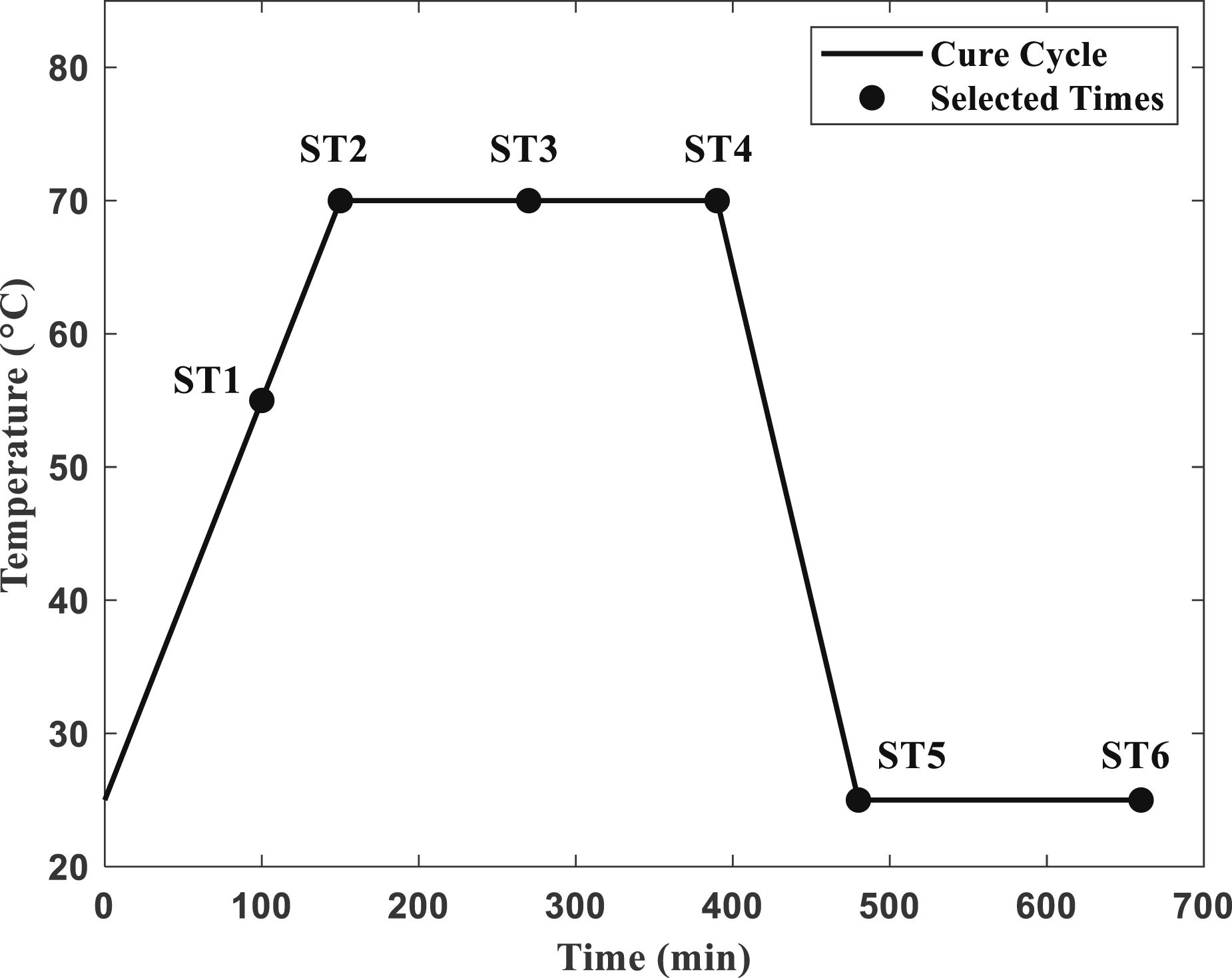

Results and discussion

The six previously mentioned scenarios are numerically simulated using VIsim, and the simulation results are organized and presented in two separate subsections. Subsection ‘Mold filling, flushing, and bleeding stages' focuses on the simulation results of the mold filling, flushing, and bleeding stages, while subsection ‘Curing stage' delves into the simulation results specifically related to the curing stage.

Mold filling, flushing, and bleeding stages

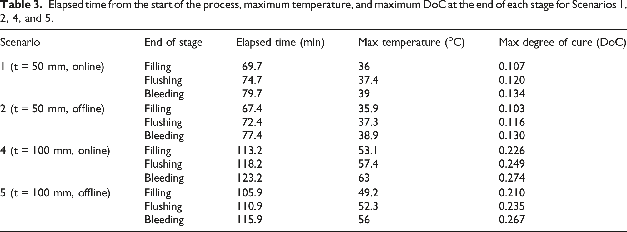
As discussed before, the mold filling, flushing, and bleeding stages are simulated for Scenarios 1, 2, 4, and 5. Table 3 provides a summary of the time elapsed from the start of the mold-filling stage, the maximum temperature, and the maximum DoC attained at the end of each stage for Scenarios 1, 2, 4, and 5.

Table 3.

Elapsed time from the start of the process, maximum temperature, and maximum DoC at the end of each stage for Scenarios 1, 2, 4, and 5.

Scenario	End of stage	Elapsed time (min)	Max temperature (^oC)	Max degree of cure (DoC)
1 (t = 50 mm, online)	Filling	69.7	36	0.107
	Flushing	74.7	37.4	0.120
	Bleeding	79.7	39	0.134
2 (t = 50 mm, offline)	Filling	67.4	35.9	0.103
	Flushing	72.4	37.3	0.116
	Bleeding	77.4	38.9	0.130
4 (t = 100 mm, online)	Filling	113.2	53.1	0.226
	Flushing	118.2	57.4	0.249
	Bleeding	123.2	63	0.274
5 (t = 100 mm, offline)	Filling	105.9	49.2	0.210
	Flushing	110.9	52.3	0.235
	Bleeding	115.9	56	0.267

Thick-section laminate (50 mm)

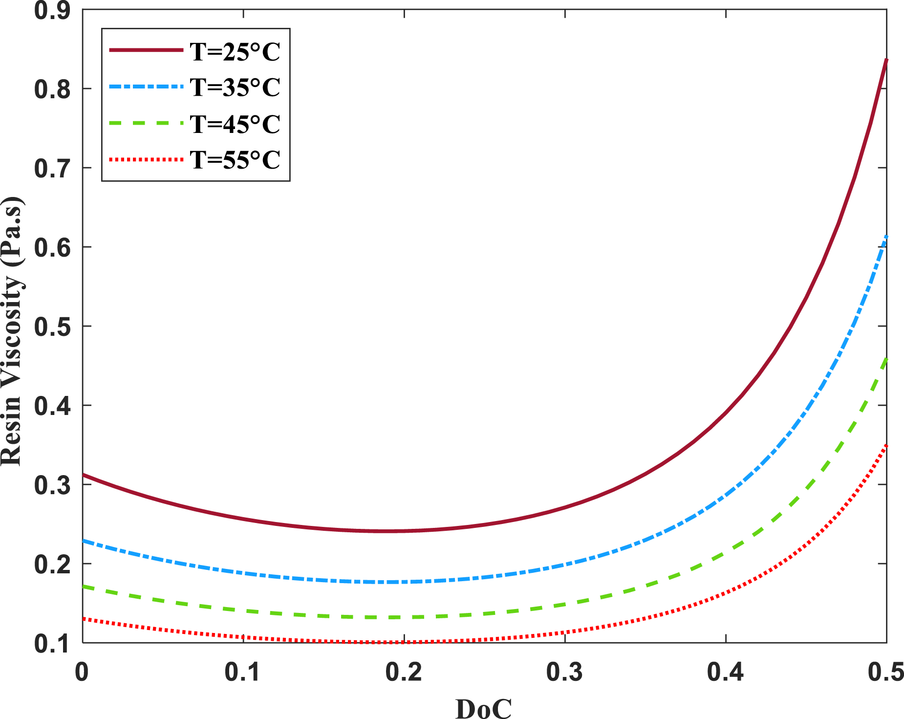
For the 50 mm thick laminate utilizing the online resin-mixing method (Scenario 1), the mold-filling stage takes 69.7 minutes. Figure 3(a) depicts the filling time contour plot for this scenario, which reveals that when the resin reaches the bottom of the laminate (the dark blue region in the figure), it has progressed 0.35 m at the top. This observation can be attributed to the significant thickness of the laminate and the implementation of a flow mesh at the top. The mold-filling pattern for Scenario 2 is similar to Scenario 1 (for brevity, not shown here). As indicated in Table 3, the mold filling time for Scenario 2 is 67.4 minutes, which is 2.3 minutes shorter than the time observed in Scenario 1. This difference can be attributed to the lower resin viscosity in Scenario 2 compared to Scenario 1. Figure 3(b) and 3(c) provide the resin viscosity contour plots at the end of the mold-filling stage for Scenarios 1 and 2, respectively. The maximum resin viscosity is found to be 0.311 Pa·s for Scenario 1, whereas Scenario 2 exhibits a lower maximum viscosity of 0.268 Pa·s, which contributes to the faster filling time observed in this scenario. When the Airston resin system undergoes curing under isothermal conditions, an initial decrease in resin viscosity is observed until the DoC attains a value of approximately 0.2. Following this point, the resin viscosity starts to increase, as depicted in Figure 4. This observation can explain why the maximum resin viscosity for Scenario 2 (offline resin mixing) is lower than that for Scenario 1 (online resin mixing). The initial decrease in Airstone resin viscosity (Equation (5)) during isothermal curing is an unusual behavior that may stem from two potential causes: (1) a physical phenomenon inherent to the resin system or (2) an unintended temperature rise during the isothermal tests reported in Ref. 28. It is important to note that during the VI process using offline resin mixing, an unmodeled factor may contribute to viscosity reduction in the early phases of resin curing. While our simulations assumed a constant 25°C inlet temperature during filling and flushing (for offline resin mixing), actual conditions would involve temperature increase at the inlet (dependent on resin pot geometry/size) alongside DoC changes. This unmodeled temperature rise would further reduce viscosity in the early curing stages. Figure 3(d) displays the resin pressure contour plot for Scenario 1 at the end of the mold-filling stage. The contour plot demonstrates the variation in resin pressure, which spans from 100 kPa at the inlet to 0 kPa at the outlet. Figure 3(e) presents the corresponding fiber volume fraction contour plot, ranging from 0.42 at the inlet to 0.52 at the outlet location due to the non-uniform distribution of compaction pressure.

Figure 3.

Filling time, viscosity, resin pressure, and fiber volume fraction contour plots for the thick laminate. (a) filling time contour plot for Scenario 1, (b) viscosity contour plot for Scenario 1 (end of mold filling), (c) viscosity contour plot for Scenario 2 (end of mold filling), (d) resin pressure contour plot for Scenario 1 (end of mold filling), (e) fiber volume fraction contour plot for Scenario 1 (end of mold filling), (f) resin pressure contour plot for Scenario 1 (end of bleeding), (g) fiber volume fraction contour plot for Scenario 1 (end of bleeding).

Figure 4.

Resin viscosity versus DoC under isothermal condition for different temperatures.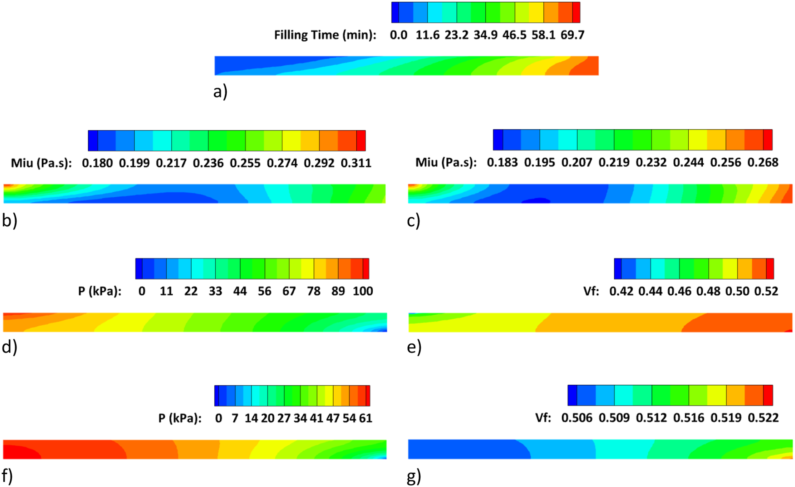

During the bleeding stage, the closure of the inlet hose leads to a decrease in resin pressure at the inlet location, ultimately enabling the pressure field to attain an equilibrium state if given adequate time. In the present study, a duration of 5 minutes is designated for the bleeding stage. The resin pressure and corresponding fiber volume fraction contour plots at the end of the bleeding stage are presented in Figure 3(f) and 3(g), respectively. As it is evident in Figure 3(f), the resin pressure at the end of the bleeding stage exhibits a range from 61 kPa at the inlet to 0 kPa at the outlet. This indicates that equilibrium has not been achieved, likely due to the restricted duration of the bleeding stage. As a result, the fiber volume fraction contour plot, displayed in Figure 3(g), spans from 0.51 at the inlet to 0.52 at the outlet.

The compaction behavior of the reinforcement significantly influences the fiber volume fraction distribution at the end of the bleeding stage. Ideally, a wet compaction model would be employed to accurately simulate this stage. However, due to insufficient data availability, the current study resorted to utilizing a wet relaxation (unloading) model of the reinforcement to approximate the behavior during the bleeding stage. The resin pressure and fiber volume fraction contour plots for Scenario 2 are similar to those in Scenario 1. Due to the similarities between the two scenarios, the contour plots for Scenario 2 are omitted for conciseness.

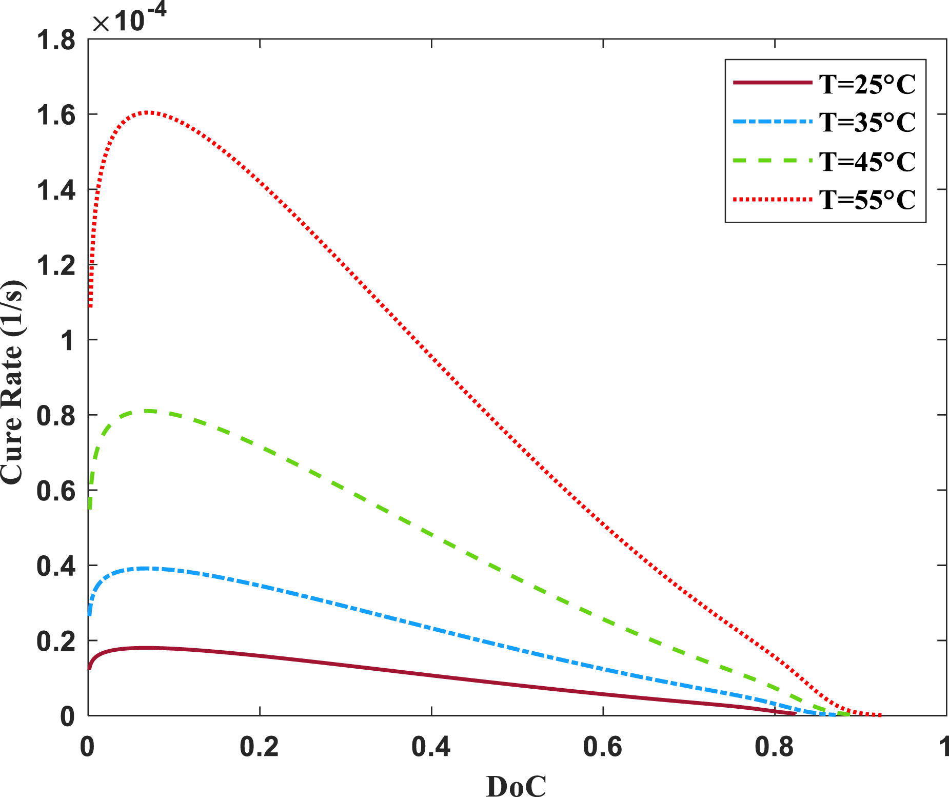
Figure 5 presents the temperature and DoC contour plots at the end of each stage (i.e., mold filling, flushing, and bleeding) for the first and second scenarios. Although the DoC contour plots (Figure 5(b) and 5(d)) differ between the first and second scenarios, the temperature contour plots (Figure 5(a) and 5(c)) are very similar. Following the specified thermal boundary condition, the temperature at the inlet location is maintained at a constant level of 25°C for both scenarios. At the end of the bleeding stage, the maximum temperature observed within the laminate is approximately 39°C for both scenarios. Figure 6 shows that at both T = 25°C and T = 35°C, the cure rate is largely independent of the DoC during the initial resin curing stages, especially for DoC values below 0.2. By increasing temperature, both the cure rate and its dependency on the DoC are increased. Since the maximum temperature and DoC magnitudes at the end of the bleeding stage for these two scenarios are 39°C and 0.134, respectively, the similarity in temperature contour plots of these scenarios is reasonable. Another important point here is that the temperature inside the mold increases up to 14°C above the ambient temperature (25°C) by the end of the bleeding stage.

Figure 5.

Temperature and DoC contour plots at the end of mold filling, flushing, and bleeding stages (from top to bottom) for Scenarios 1 and 2. (a) temperature contour plots for Scenario 1, (b) DoC contour plots for Scenario 1, (c) temperature contour plots for Scenario 2, (d) DoC contour plots for Scenario 2.

Figure 6.

Relationship between the cure rate of the resin and DoC under isothermal conditions for various temperatures.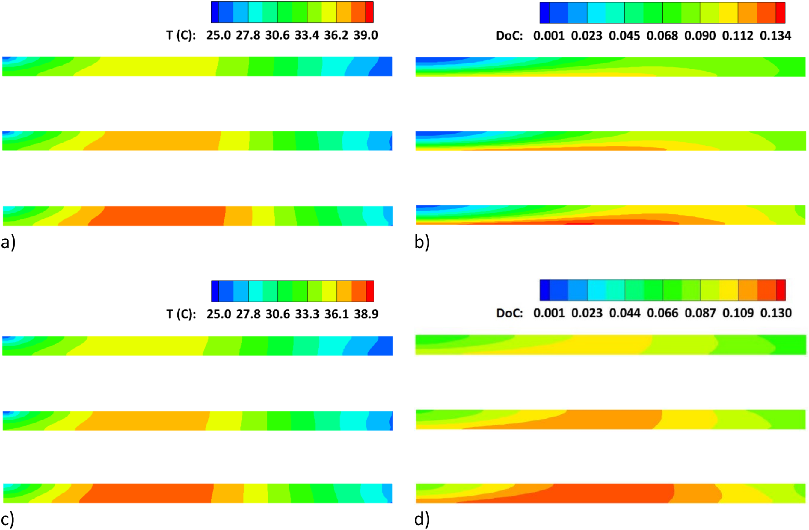

As anticipated, due to using different resin-mixing types, the DoC contour plots for Scenarios 1 and 2 are different, although they are similar near the outlet location (see Figure 5(b) and 5(d)). At the end of the bleeding stage, the largest DoC gradient in the thickness direction occurs in Scenario 1 (online resin mixing) near the inlet location (Figure 5 (b)). In Scenario 1, the region with the highest DoC forms a tape-like shape at the bottom of the laminate. This region spans from the vicinity of the inlet until after the center of the laminate. In Scenario 2, the highest DoC region maintains the same longitudinal position as in Scenario 1. However, it differs in its distribution across the thickness, as it spans the entire thickness of the laminate at its center. Using equation (6) for the resin’s cure kinetics at ambient temperature and considering the elapsed time until the end of the bleeding stage for Scenario 1 (79.7 min) and Scenario 2 (77.4 min) (see Table 3), the DoCs are calculated as 0.083 and 0.081, respectively. However, according to Figure 5(b) and 5(d), the maximum DoC magnitudes at the end of the bleeding stage for Scenarios 1 and 2 are 0.134 and 0.130, respectively. These values are 61.4% and 60.5% higher than the DoCs calculated using equation (6).

Ultra-thick-section laminate (100 mm)

The mold filling pattern for Scenario 4 is similar to Scenario 1; however, the resin advances 0.65 m at the top before reaching the laminate’s bottom, and it is almost doubled compared to 0.35 m in Scenario 1. The mold-filling times for the fourth and fifth scenarios are 113.2 minutes and 105.9 minutes, respectively. By employing the offline resin-mixing method, the mold filling time is reduced by 7.3 minutes compared to the online resin-mixing approach. Similar to the thick laminates discussed earlier, the reduction in filling time for Scenario 5 compared to Scenario 4 can be attributed to the lower maximum viscosity value observed in Scenario 5 (0.252 Pa·s) as opposed to Scenario 4 (0.311 Pa·s). The resin pressure and fiber volume fraction contour plots at the end of the mold filling and bleeding stages for ultra-thick laminates exhibit similar ranges to those observed in thick laminates, as previously discussed. In the interest of conciseness, the contour plots representing filling time, resin viscosity, resin pressure, and fiber volume fraction for ultra-thick laminates have not been presented.

Figure 7 presents the temperature and DoC contour plots at the end of each stage for Scenarios 4 and 5. The maximum temperatures at the end of the bleeding stage are 63°C and 56°C for Scenarios 4 and 5, respectively. In other words, at the end of the bleeding stage, the temperature inside the mold experiences an increase of 38°C and 31°C above ambient temperature for the online and offline resin-mixing schemes, respectively. The temperature distribution patterns in the contour plots are relatively similar for Scenarios 4 and 5. The higher maximum temperature observed in Scenario 4 compared to Scenario 5 can be partially attributed to the longer mold filling time required in Scenario 4.

Figure 7.

Temperature and DoC contour plots at the end of mold filling, flushing, and bleeding stages (from top to bottom) for Scenarios 4 and 5. (a) temperature contour plots for Scenario 4, (b) DoC contour plots for Scenario 4, (c) temperature contour plots for Scenario 5, (d) DoC contour plots for Scenario 5.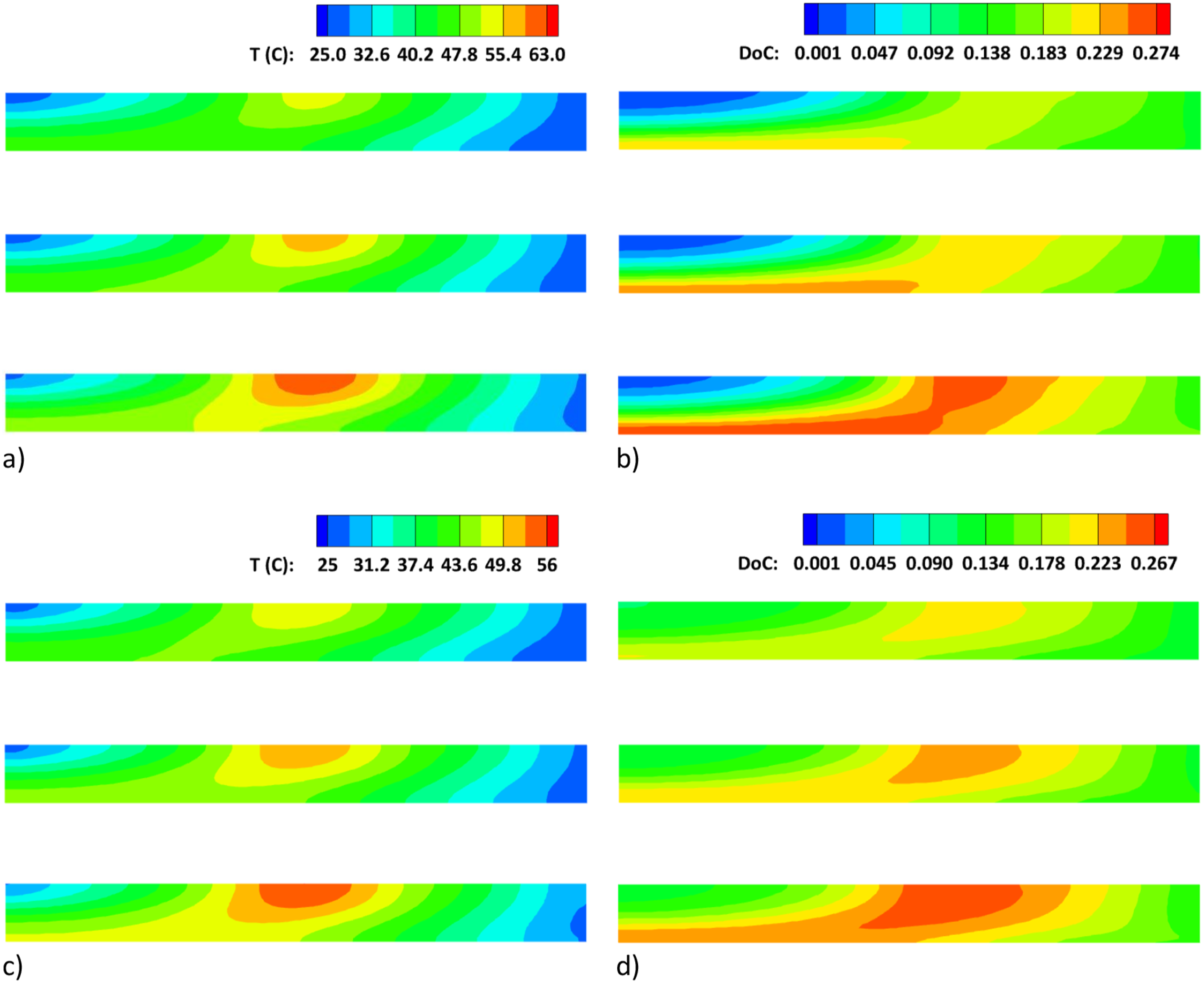

Comparing the highest DoC regions in Scenarios 4 and 5, it can be observed that Scenario 4 exhibits a region that extends from the center upper part of the laminate towards the lower section of the left edge. On the other hand, Scenario 5 displays the highest DoC region concentrated at the upper portion of the laminate’s center. The DoC contour plots for both scenarios are similar near the outlet location. At the end of the bleeding stage, the largest DoC gradient in the thickness direction is associated with Scenario 4 (online resin-mixing type) near the inlet location. Using equation (6) for the resin’s cure kinetics at ambient temperature and considering the elapsed time until the end of the bleeding stage for Scenario 4 (123.2 min) and Scenario 5 (115.9 min), the DoCs are calculated as 0.130 and 0.122, respectively. However, based on Figure 7(b) and 7(d), the maximum DoC magnitudes at the end of the bleeding stage for Scenarios 4 and 5 are 0.274 and 0.267, respectively. These values are 110.8% and 118.9% higher than the DoCs calculated using equation (6).

Comparison of simulation results for thick and ultra-thick laminates

Comparing the mold-filling times under both online and offline resin mixing techniques reveals a 62.4% and 55.8% increase for the ultra-thick laminate compared to the thick laminate, respectively (see Table 3).

As previously discussed, the resin progresses 0.35 m and 0.65 m forward at the top of the laminate upon reaching the bottom for Scenarios 1 and 4, respectively. This observation underscores the influence of laminate thickness on the mold-filling pattern, emphasizing the significance of selecting appropriate flow mesh length and permeability. Proper selection of these parameters is crucial to prevent the formation of voids in the laminate due to discrepancies in the lead-lag length of the flow front.

Figure 8(a) and 8(b) illustrate the laminate thickness evolution at locations a, b, c, d, and e (refer to Figure 1) from the beginning of the process until the end of the bleeding stage for Scenarios 1 and 4, respectively. During the mold-filling stage, the laminate thickness consistently increases at all five locations. Throughout the flushing stage, the thickness remains relatively stable, with only minor decreases observed at locations a and b. Finally, the bleeding stage witnesses a decrease in thickness across all five locations. Notably, the laminate thickness at location a experiences a maximum increase of up to 4 mm for the thick laminate and 5.6 mm for the ultra-thick laminate.

Figure 8.

Thickness history of the thick and ultra-thick laminates at a, b, c, d, and e locations (see Figure 1) for (a) Scenario 1 and (b) Scenario 4.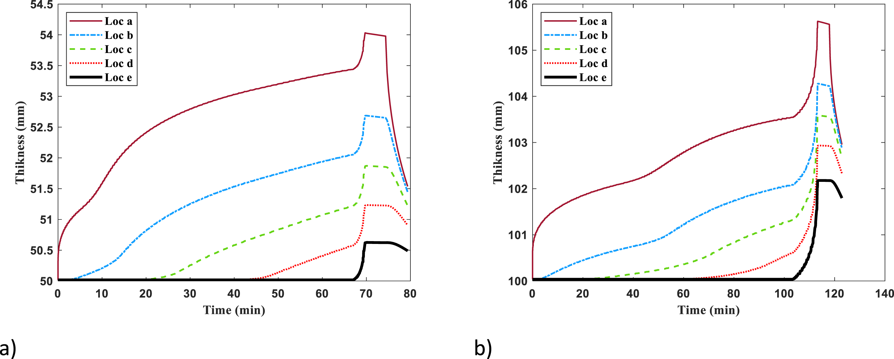

It should be noted that the laminate thickness values observed during the bleeding stage may not be reliable because the wet relaxation (unloading) model is used instead of the wet compaction model for modeling the compaction behavior of the reinforcement in this stage. Furthermore, as highlighted by certain researchers,^34,35 it is crucial to account for the time-dependent behavior of the reinforcement in the thickness direction to accurately determine the thickness distribution along the laminate at the end of the process.

At the end of the bleeding stage, the maximum temperatures within the thick (Scenario 1) and ultra-thick (Scenario 4) laminates are 39°C and 63°C, respectively. This demonstrates that the maximum temperature for the ultra-thick laminate is 24°C higher than that for the thick laminate. Moreover, the difference between the maximum and minimum temperatures within the thick laminate is 14°C, whereas this difference increases to 38°C for the ultra-thick laminate. Temperature variations within the mold can affect the curing and evolution of residual stress. These effects will be discussed in subsequent sections.

The temperature distribution patterns are different for the thick and ultra-thick laminates, indicating that the thickness of the laminate, the mold filling pattern with resin, and the mold filling time have crucial effects on the temperature distribution within the mold. For the thick laminate, the highest temperature region extends across the thickness from the second quarter of the sample length up to the center of the laminate. In contrast, the ultra-thick laminate exhibits a concentrated high-temperature region at the top center of the laminate.

At the end of the bleeding stage, the maximum DoC within the thick laminate (Scenario 1) is 0.134, while for the ultra-thick laminate (Scenario 4), it reaches 0.274. Therefore, the maximum DoC for the ultra-thick laminate is 104.5% higher than the thick laminate. Comparing the highest DoC regions for Scenarios 4 and 1, it can be observed that the region in Scenario 4 is quite similar to that in Scenario 1, with an additional region that extends through the thickness at the center of the ultra-thick laminate.

The resin-mixing method significantly affects the DoC distribution in both thick and ultra-thick laminates. However, the influence of the resin-mixing type on temperature distribution varies between the two laminate types. For thick laminates, the impact is found to be insignificant, whereas for ultra-thick laminates, the resin-mixing type has a considerable effect on temperature distribution.

Curing stage

In this section development of the residual stresses and resulting deformations during the curing process for the thick and ultra-thick laminates under the introduced six scenarios is discussed. Due to the significant number of fabric layers in both thick and ultra-thick laminates, an equivalent stiffness matrix is employed to model the laminate as a single orthotropic material. This matrix is derived by averaging the stiffness matrices for the 0 and 90-degree plies, as discussed in Section ‘Six scenarios for numerical investigation'. This simplification enables the evolution of residual stress to be solely dependent on the temperature and DoC histories within the laminate, without the influence of variations in material properties across adjacent layers. Therefore, the residual stress development within the laminates can be attributed to the following three main factors: spatial variations in material properties (chemical hardening), chemical shrinkage, and thermal shrinkage/expansion.³⁶ These individual contributors interact and accumulate, resulting in the residual stress distribution observed within the laminate.

To study the evolution of residual stress within the laminates, it is necessary to investigate the histories of spatial variations in resin modulus (representing chemical hardening), DoC (representing chemical shrinkage), and temperature (representing thermal shrinkage/expansion). The residual stress within the laminates exhibits variations in both longitudinal and thickness directions. The subsequent subsections will delve into the evolution of longitudinal residual stresses within thick and ultra-thick laminates. Additionally, the development of interlaminar normal residual stresses along the left and right edges of the laminates will be examined. Furthermore, the deformation of the laminates at the end of the curing stage will be investigated, providing a comprehensive understanding of the laminate’s behavior during the curing stage.

Thick-section laminate (50 mm)

Analysis of longitudinal residual stress evolution

Figure 9(a), 9(c), and 9(e) (corresponding to Scenarios 1, 2, and 3 in respect) depict the variations in longitudinal residual stress ( $σ_{1}$ ) and resin modulus (Er) along the thickness at the center of the model (TDLine, as shown in Figure 1) for the five selected times (ST2-ST6, as indicated in Figure 2). Note, the curves without square markers represent the residual stresses at times ST2-ST6, while the curves accompanied by square markers correspond to the resin modulus (Er) values at the mentioned STs. Additionally, Figure 9(b), 9(d), and 9(f) illustrate the corresponding temperature and DoC variations for Scenarios 1, 2, and 3, respectively. Here, also, the curves without square markers present the temperature distribution, and the curves with square markers illustrate the DoC of the models for the five STs. It is important to note that the longitudinal gradients in temperature, DoC, and resin modulus can also influence the distribution of residual stresses along the TDLine. In this section, the analysis of residual stress evolution is presented qualitatively.

Figure 9.

Distribution of longitudinal stress and resin modulus along the TDLine at ST2-ST6 for (a) Scenario 1, (c) Scenario 2, (e) Scenario 3, and distribution of temperature and DoC along the TDLine at ST2-ST6 for (b) Scenario 1, (d) Scenario 2, and (f) Scenario 3.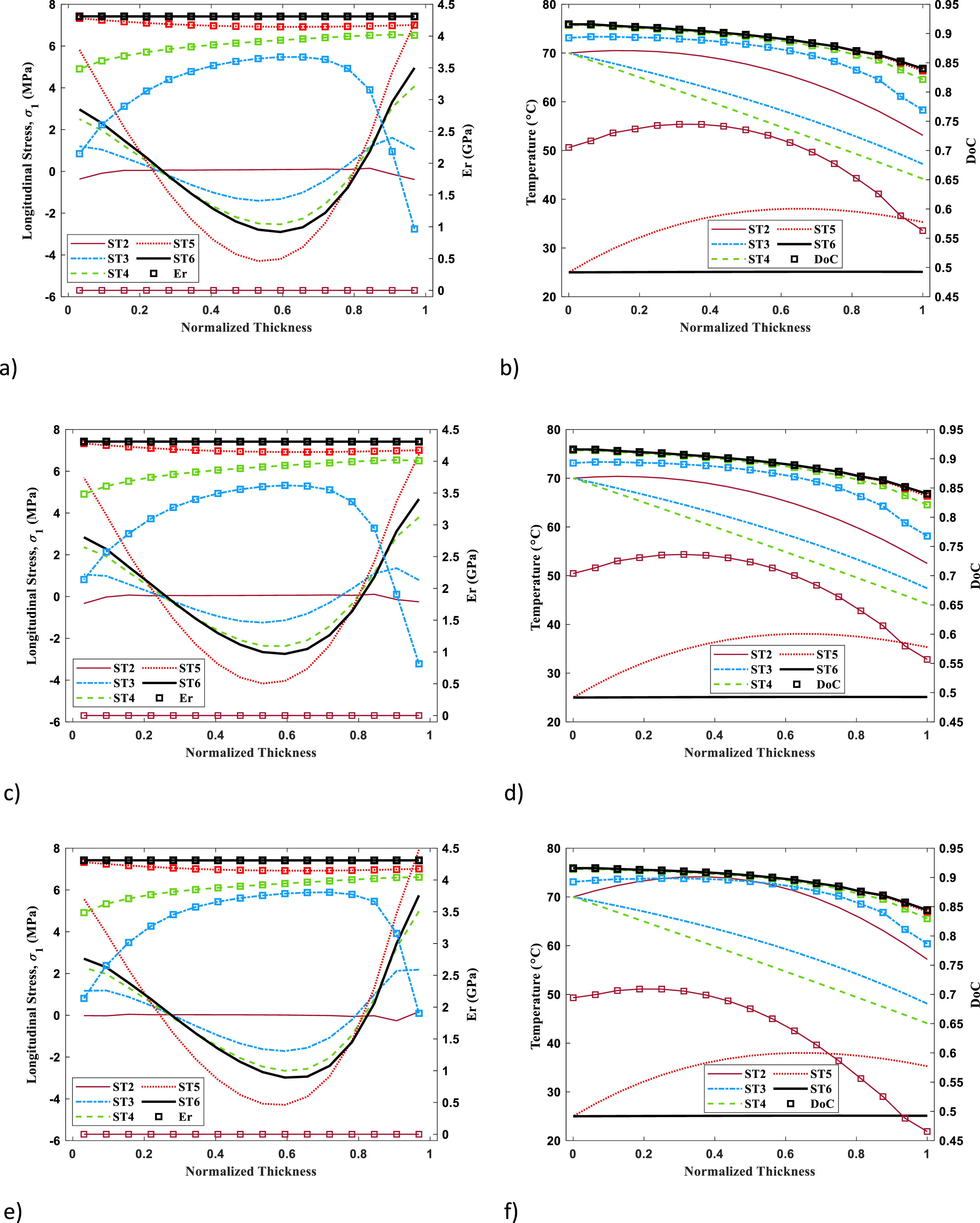

At ST2, the resin modulus is constant ( $E_{r u b}$ ) across all scenarios (Figure 9(a), 9(c) and 9(e)). At ST2, a small residual stress is observed along TDLine (passing through the thickness at the mid-length of the sample), which is tensile at mid-thickness and compressive (maximum −0.39 MPa) at both the top and bottom of the laminate. This observation suggests that the chemical shrinkage at the center region (mid-thickness) is more prominent than the chemical shrinkage at the top and bottom regions of TDLine, potentially due to the higher magnitude of DoC at the center region. For Scenario 3 (see Figure 9(e) and 9(f)), the magnitudes of residual stress at the top and bottom of TDLine are comparatively smaller and exhibit a bit different trend in comparison to the first two scenarios. In Scenario 3, the temperature distribution, with higher values at the center, differs from those for Scenarios 1 and 2. The magnitude of DoC is also lower at the top of TDLine. In Scenario 3, the temperature distribution exhibits higher values especially at the center, distinguishing it from the patterns observed in Scenarios 1 and 2. Additionally, the DoC demonstrates a lower magnitude at the top of TDLine relative to Scenarios 1 and 2. The observed distribution of longitudinal residual stress can be attributed to the interaction between chemical shrinkage and thermal expansion occurring along TDLine during the starting of the curing process up until ST2.

With the progress of the curing process from ST2 to ST3, the resin modulus exhibits non-uniform development across the thickness of the laminate (TDLine), reaching its maximum value at the center region, its minimum value at the top region, and an intermediate value at the bottom region. During this period, the chemical shrinkage exhibited along TDLine is non-uniform, with a higher magnitude at both the top and bottom of TDLine relative to the mid-thickness region, due to the larger DoC change. Thermal shrinkage also exhibits a non-uniform distribution, with a higher magnitude at the mid-thickness region than at both ends of the TDLine. However, the distribution of chemical shrinkage predominates over the thermal shrinkage distribution, determining the dominant residual stress pattern along the TDLine. Therefore, the center region offers resistance to the shrinkage of both the top and bottom regions. Consequently, tensile residual stresses are developed at both ends, while compressive residual stresses appear at the center region of the TDLine. However, for Scenario 3, the DoC change at the top region is significantly greater than that at the bottom region. Furthermore, at ST3, the resin modulus of the top region is higher than those observed in the first two scenarios. These factors result in a greater tensile stress at the top region relative to the bottom region. In addition, the location of maximum compressive stress is slightly displaced from the center region to the top region of the thickness.

From ST3 and ST4, the resin modulus increases significantly along the entire thickness, particularly at the top and bottom regions. A small temperature gradient is observed, exhibiting higher values at the center and top regions compared to the bottom of TDLine. Chemical shrinkage predominates, with higher magnitudes at both ends, particularly the top region, due to the greater DoC change. Consequently, the development of tensile residual stresses at the top and bottom regions, and compressive residual stresses in the central region can be observed. Throughout this period, the tensile residual stress generated at the top region is more substantial than that at the bottom region. This disparity can be attributed to the collective impact of a higher resin modulus and a more significant DoC change occurring in the top region as compared to the bottom region. Additionally, the location of maximum compressive residual stress shifts slightly to the top region. It should be noted that due to a proper development of resin modulus along TDLine, thermal shrinkage along TDLine can also play a minor role in inducing tensile and compressive stresses at the top and bottom regions, respectively.

From ST4 to ST5, the resin modulus increases in the entire thickness, especially at the bottom region. There is a small chemical shrinkage at the top region, while thermal shrinkage occurs throughout the thickness, particularly dominating at the bottom region. As a result, shrinkage prevails at the bottom of TDLine. This leads to a significant increase in tensile and compressive residual stresses at the bottom and center regions of TDLine, respectively. Furthermore, the maximum compressive residual stress shifts to the bottom side. The development of substantial tensile stresses at the top of TDLine arises to satisfy the equilibrium condition, which stipulates that the summation of longitudinal residual stresses along TDLine must equal zero.

From ST5 to ST6, as the laminate cools down, the resin modulus increases along the entire thickness. Thermal shrinkage is also dominant at the center and top regions. This results in the development of tensile and compressive residual stresses at the center and bottom of TDLine, respectively. Therefore, the maximum compressive residual stress shifts slightly to the top region. In response to the need for maintaining equilibrium, the laminate’s longitudinal stress distribution along TDLine adapts, resulting in the development of significant compressive stresses at the top of TDLine.

The longitudinal residual stresses within the laminate exhibit variation along both the thickness and longitudinal directions of the laminate. To study the variation in the longitudinal direction, five sensing points (labeled a, b, c, d, and e as shown in Figure 1), which are located on the mid-thickness and at equidistance along the longitudinal direction, are considered. Figure 10(a), 10(c), and 10(e) present the temperature history and Tg evolution of the resin at SPs a–e during curing for Scenarios 1–3, respectively. In these figures, graphs with square markers represent Tg, while those without markers denote temperature. The corresponding evolution of resin modulus and longitudinal residual stresses for the initial three scenarios are depicted in Figure 10(b), 10(d), and 10(f), respectively. In these figures, graphs with square markers represent Er, while those without markers represent the longitudinal stress.

Figure 10.

Time histories of temperature and Tg for (a) Scenario 1, (c) Scenario 2, (e) Scenario 3, and time histories of longitudinal stress and resin modulus for (b) Scenario 1, (d) Scenario 2, and (f) Scenario 3 at sensing points (SPs) labeled a-e during the curing stage.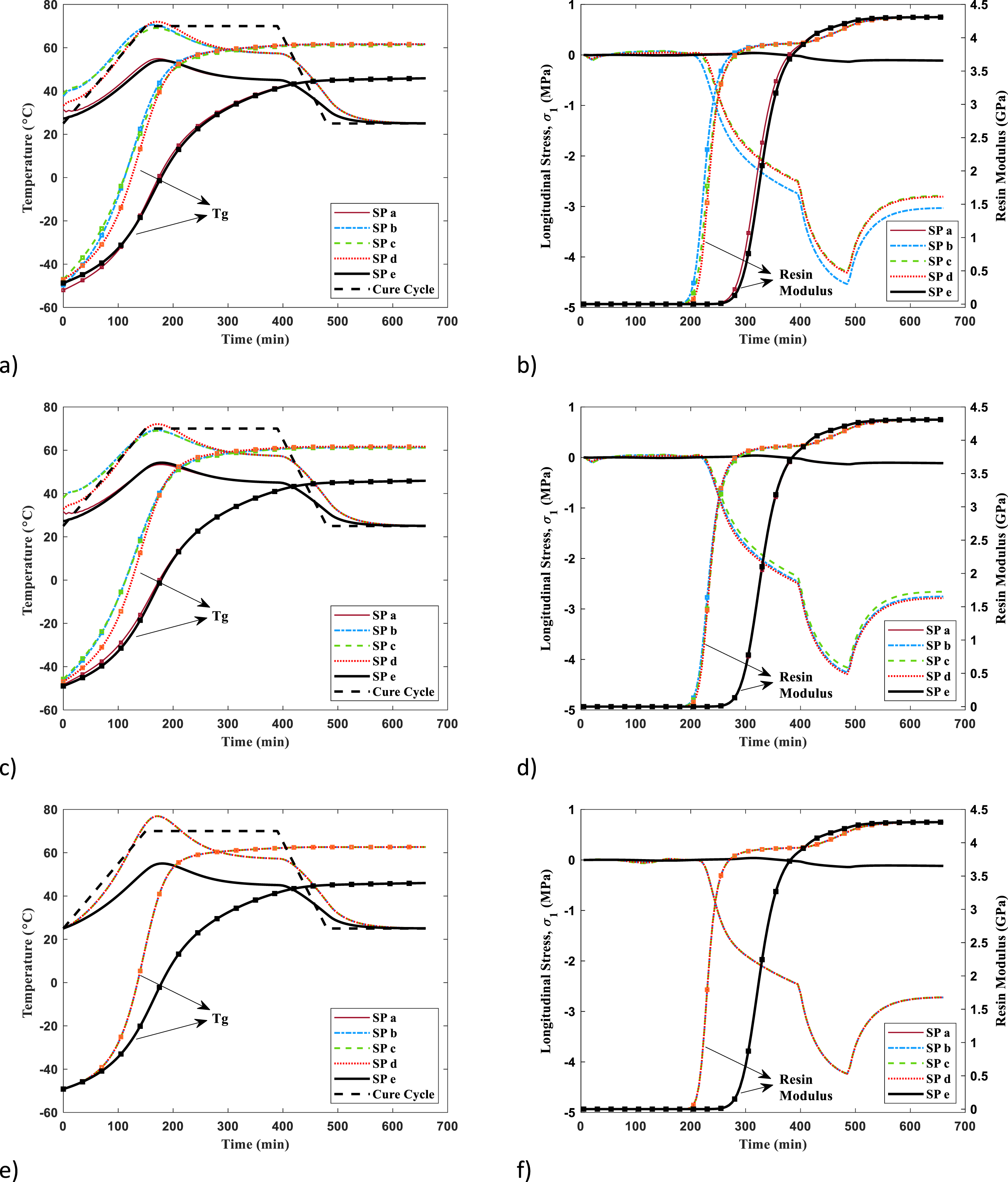

As illustrated in Figure 10(a), 10(c), and 10(e), for all three scenarios, the temperature at all five SPs increases until slightly after the transition to the holding phase at 70°C during the cure cycle. Following this point, the temperature at all five SPs gradually decreases throughout the subsequent phases of the cure cycle, which include holding at 70°C, cooling, and holding at 25°C. The temperature rise at SPs a and e is smaller than at other SPs due to increased heat convection with the ambient environment. The maximum temperature is recorded at SP d with a peak value of 76.9°C for Scenario 3 and 72°C for Scenarios 1 and 2. In Scenario 3, the temperature histories at SPs b, c, and d are identical due to the same initial conditions of temperature and DoC within the laminate, as well as their location being sufficiently distant from the left and right edges. Additionally, the temperature histories at SPs a and e are also identical.

The evolution of the glass transition temperature (Tg) is directly linked to the DoC progression, as defined by equation (7). By examining Figure 10, it becomes apparent that when the difference between the temperature and Tg at a specific SP within the laminate decreases to approximately 25°C, the resin modulus begins to increase significantly, which is in full agreement with that reported in Ref. 15. Across all three scenarios, the resin modulus initially develops for the three central SPs (b, c, and d) prior to the two edge SPs (a and e). Although slight variations exist in the start time of resin modulus enhancement across all three scenarios, the resin modulus begins to sharply increase at approximately 200min and 270 min for the central and edge SPs, respectively. The considerable increase in resin modulus after the vitrification points is attributed to the cooling of the laminate. In Scenario 1, for the SPs a, b, c, d, and e, vitrification occurred at 416 min, 295 min, 300 min, 310 min, and 417.5 min, respectively. While for Scenario 2, it occurred at 417.5 min, 310 min, 313.5 min, 302 min, and 417.5 min. However, for Scenario 3, vitrification occurred at 283 min and 416.5 min for the central and edge SPs, respectively.

Across all three scenarios, behavior of longitudinal residual stresses at the central SPs (b, c, and d) exhibits similar trends (see Figure 10(b), 10(d), and f10(f)). For Scenario 1, a minor deviation of the longitudinal stress history at SP b from those of SPs c and d is attributable to the earlier development of the resin modulus at SP b. For all three scenarios, the final longitudinal residual stress at SPs a and e is equal to −0.12 MPa. This low longitudinal stress magnitude is anticipated, as these SPs are located close to the free surface of the sample ends. It is worth noting that the longitudinal residual stress magnitudes reported in the current study were read at the center of the respective elements.

While the resin modulus evolution at the five selected times (STs) has been discussed, it is important to examine the spatial evolution of the resin modulus within the laminate. This is due to the significant impact that the spatial distribution of resin modulus has on the development and spatial evolution of residual stresses throughout the laminate during the curing process. Figure 11(a)–11(c) present the resin modulus contour plots for Scenarios 1, 2, and 3 at three selected times: 220 min (after ST2), 270 min (ST3), and 390 min (ST4), respectively. Resin modulus values below 0.1 GPa are excluded from the contour plots to provide a clearer representation of the resin modulus evolution within the laminates.

Figure 11.

Contour plots of resin modulus (Er) within the thick laminate at the times of 220 min (after ST2), 270 min (ST3), and 390 min (ST4) for (a) Scenario 1, (b) Scenario 2, and (c) Scenario 3.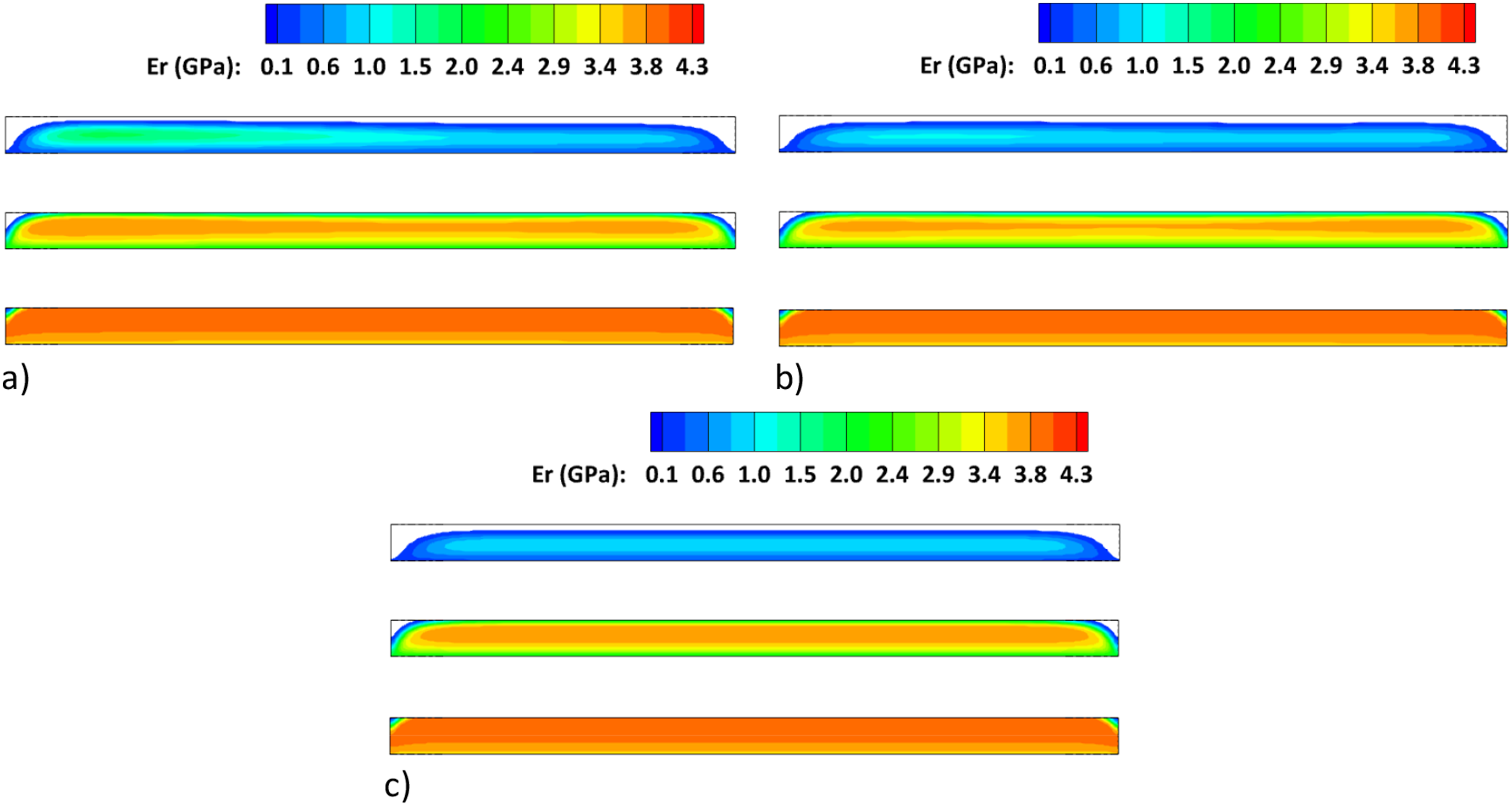

At 220 min (after ST2), when the resin modulus within the laminate is in its initial stage of development, the regions with the highest resin modulus values in the contour plots for all three scenarios correspond to the first-gelled regions within the laminate. The highest resin modulus value is observed in Scenario 1 (online resin mixing), primarily concentrated near the inlet region. Comparing the resin modulus distribution across the three scenarios, Scenario 3 exhibits a more uniform spatial distribution of resin modulus along the longitudinal direction. At ST3, the resin modulus within the central region of the laminate (for all three scenarios) has developed significantly, exhibiting variations in both the longitudinal and transverse directions. In contrast, the development of the resin modulus at SPs a and e has not yet commenced at this time instant. The resin modulus distribution at the top corners of the laminate remains underdeveloped even at ST4, indicating the slower development process of resin modulus in these regions. By the end of the process, the resin modulus distribution becomes homogeneous within the laminate for all three scenarios.

Following the analysis of the spatial evolution of resin modulus in the thick laminate, it is beneficial to examine the spatial development of longitudinal residual stresses within these laminates. Figure 12 depicts the longitudinal residual stress contour plots for the three scenarios at four key time instants (from top to bottom): ST3, ST4, ST5, and ST6, respectively.

Figure 12.

Contour plots of longitudinal residual stress within the thick laminate at four selected times (ST3, ST4, ST5, and ST6) for (a) Scenario 1, (b) Scenario 2, and (c) Scenario 3.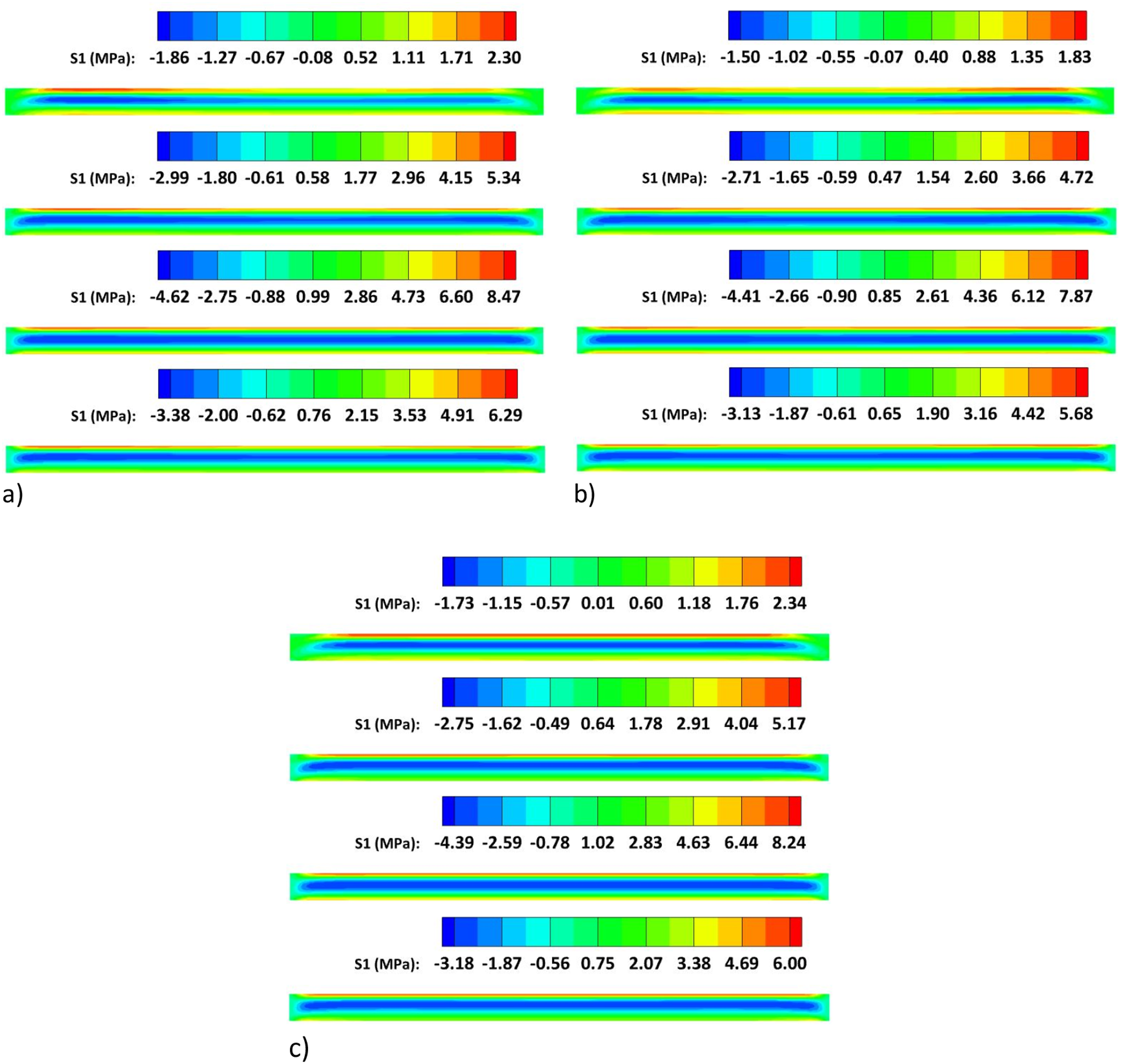

At ST3, for all three scenarios, the longitudinal residual stress is compressive within the central regions of the laminate where the resin modulus is the highest (see Figure 11). Additionally, tensile longitudinal residual stresses are observed at the top and bottom regions of the laminate. In contrast to Scenario 3, where uniform residual stresses are observed along the longitudinal direction, the residual stress distributions in Scenarios 1 and 2 exhibit non-uniformity due to variations in resin modulus within the central regions of the laminate. At the regions near the right and left edges, the residual longitudinal stress is insignificant due to the presence of free surfaces.

While the magnitudes of residual stresses vary at different STs, the nature of these stresses remains consistent across all STs, with compressive residual stresses prevailing in the central region and tensile residual stresses present at both the top and bottom regions of the laminate. The maximum tensile and compressive longitudinal residual stresses (in MPa) experienced by the laminate during the curing process (corresponding to ST5) are 8.47 and 4.62 for Scenario 1, 7.87 and 4.41 for Scenario 2, and 8.24 and 4.39 for Scenario 3, respectively. Therefore, the maximum tensile and compressive longitudinal residual stress experienced within the thick laminate during the curing stage is associated with Scenario 1, in which the online resin mixing scheme is used.

At the end of the curing process, the tensile and compressive longitudinal stresses (in MPa) within the laminate are 6.29 and 3.38 for Scenario 1, 5.68 and 3.13 for Scenario 2, and 6.00 and 3.18 for Scenario 3, respectively. Therefore, the maximum tensile and compressive longitudinal residual stress experienced within the thick laminate at the end of the curing stage is also associated with Scenario 1.

Analysis of interlaminar normal residual stress evolution

Interlaminar stresses are critical in composite laminates with free edges because they may cause delamination. Free surfaces and property variations between adjacent layers generate significant interlaminar normal and shear stresses at the edges. Near these locations in the laminate, to maintain equilibrium between the moment generated by the interlaminar normal stress (along the out-of-plane axis) and the corresponding moment produced by the in-plane longitudinal stress, the interlaminar normal stress must be non-zero in the region close to the edge. Figure 13(a)–13(c) depict the interlaminar normal stress at the right edge (RE) and left edge (LE) of the laminate at five selected times (ST2, ST3, ST4, ST5, and ST6) for Scenarios 1, 2, and 3, respectively.

Figure 13.

The interlaminar normal stress distributions at the right edge (RE) and left edge (LE) of the thick laminate at five selected times (ST2, ST3, ST4, ST5, and ST6) for (a) Scenario 1, (b) Scenario 2, (c) Scenario 3, and (d) the interlaminar normal stress distributions along LDLine for Scenarios 1, 2, and 3.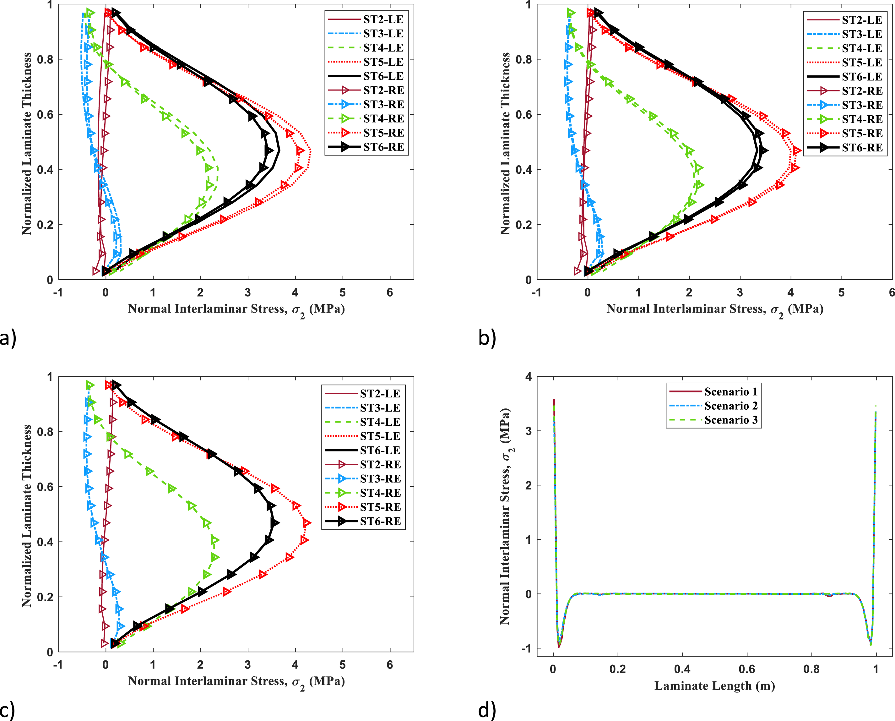

At the end of the curing stage, tensile interlaminar normal stresses are expected at the right and left edges due to moment balancing, since longitudinal stresses in the top and bottom of the laminate are tensile in these areas. However, the magnitude of the longitudinal compressive stress in the central region and its associated moment are comparatively small. For a better understanding, the reader may consider isolating a segment of the laminate in the top corner and visualizing the longitudinal and interlaminar normal stresses acting upon it.³⁷

At ST3, the development of the resin modulus near the right and left edges of the laminate occurs predominantly on the lower half-thickness of the laminate, as observed in Figure 11. The bottom of the laminate experiences tensile longitudinal stress, while a compressive longitudinal stress region exists above and close to it. As the distance from the bottom edge of the laminate increases, the moment generated by the compressive stress becomes more dominant compared to the moment generated by the tensile stress. As a result, the interlaminar normal stress experiences a shift from tensile to compressive, as demonstrated in Figure 13(a)–13(c).

At ST4, the interlaminar normal stress has developed as a consequence of the increased magnitudes of the resin modulus and longitudinal stresses in the regions near the edges of the laminate. However, the resin modulus has not yet been well developed close to the top corners of the laminate (see Figure 11).

At ST5, the interlaminar normal stresses at the right and left edges of the laminate reach their maximum magnitudes, i.e. 4 MPa and 4.2 MPa for Scenario 1, 4.1 MPa and 4.3 MPa for Scenario 2, and 4.2 MPa for Scenario 3 as observed in Figure 13, respectively.

At ST6, the decrease in longitudinal stresses causes a corresponding reduction in the interlaminar normal stresses. The maximum magnitudes of interlaminar normal stresses at the end of the curing stage are 3.2 MPa and 3.5 MPa for Scenario 1, 3.1 MPa and 3.3 MPa for Scenario 2, and 3.2 MPa for Scenario 3 at the right and left edges, respectively. Comparing these values, it is observed that the maximum interlaminar normal stresses during and at the end of the curing stage belong to Scenario 2 (i.e., 4.3 MPa) and Scenario 1 (i.e., 3.5 MPa), respectively. This result highlights the influence of the resin mixing scheme on the development of these stresses.

Figure 13 shows that Scenario 1 exhibits the largest difference in interlaminar normal stresses between the right and left edges among the three scenarios across all STs, which may be attributed to the DoC distribution within the laminate at the beginning of the curing stage. As seen in Figure 5(b), at the beginning of the curing stage, Scenario 1 displays the maximum DoC gradient in the thickness direction near the inlet location, which is attributed to the utilization of the online resin mixing scheme in this scenario.

Figure 13(d) also illustrates the distribution of interlaminar normal stress along the LDLine (see Figure 1) at the end of the curing process for Scenarios 1, 2, and 3. This figure indicates that the compressive interlaminar normal stress has become requisite behind the tensile interlaminar normal stress, to satisfy the equilibrium condition.

Analysis of curing quality and process-induced deformation

According to Figure 14, at the end of the curing stage, DoC distributions for all three scenarios exhibit high similarity. The maximum DoC values across all three scenarios (1, 2, and 3) are identical, which is equal to 0.918 at the bottom of the laminates. Moreover, minimum DoC values are observed at the top corners of the laminates for Scenarios 1, 2, and 3 with the values of 0.737, 0.743, and 0.744, respectively.

Figure 14.

Contour plots of DoC within the thick laminate at the end of the curing stage for (a) Scenario 1, (b) Scenario 2, and (c) Scenario 3.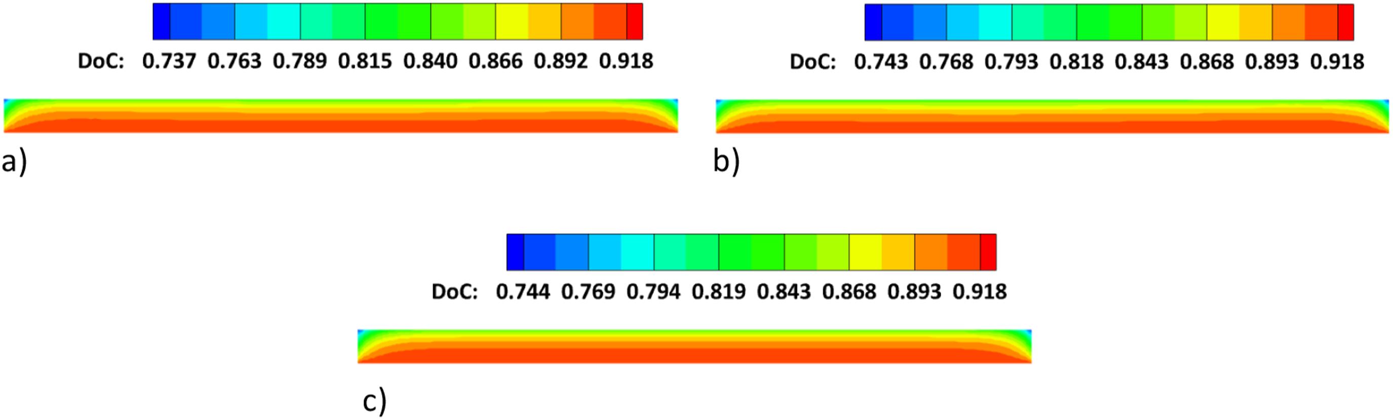

Figure 15(a)–15(c) present the contour plots of horizontal and vertical displacement components (U1 and U2) of the deformed laminates at the end of the curing stage for Scenarios 1, 2, and 3, respectively. Deformations are exaggerated fivefold for clarity. It is essential to highlight that the deformations presented reflect the cumulative deformations from the processing minute of 180 right after the beginning of the curing process until its conclusion. The resin modulus within thick laminates starts to enhance significantly from the same time point, i.e. 180 minutes after the cure initiation (see Figure 10(b), 10(d), and 10(f)). That is why the deformation of laminates before this time point is ignored.

Figure 15.

Contour plots of the displacement components (U1 and U2) of the deformed thick laminate at the end of the curing stage for (a) Scenarios 1, (b) Scenario 2, and (c) Scenario 3.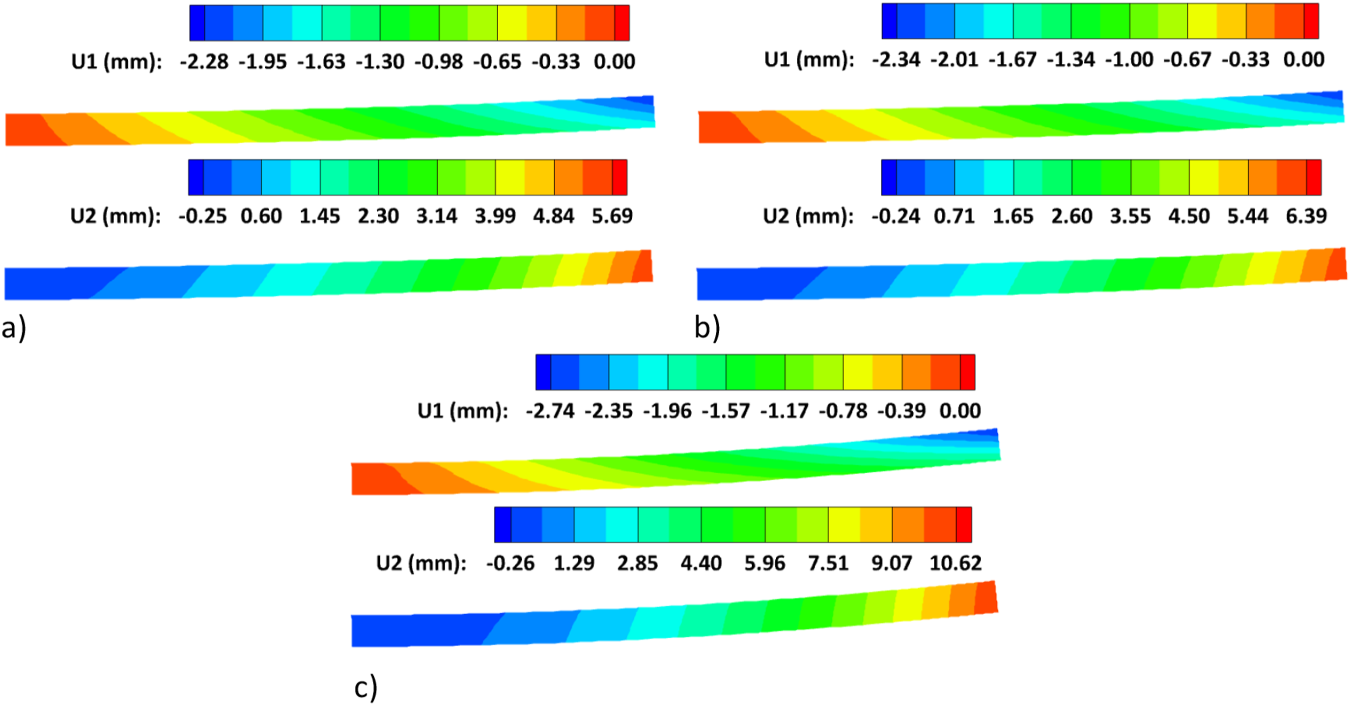

Upon examination of the contour plot of displacement components, it becomes evident that Scenarios 1–3 display similar deformation patterns; however, there are notable differences in the maximum vertical and horizontal displacement magnitudes at the right edges of the laminates. The maximum vertical/horizontal displacements of 5.69 mm/−2.28 mm, 6.39 mm/−2.34 mm, and 10.62 mm/−2.74 mm, for Scenarios 1, 2, and 3, in respect, demonstrate the substantial influence of non-uniform temperature and DoC distributions, as well as resin-mixing types on displacement evolution during the curing process. The maximum vertical displacement experienced within the thick laminate at the end of the curing stage is associated with Scenario 3, in which the uniform DoC and temperature fields with lower magnitudes are used at the beginning of the curing stage. Therefore, it is crucial to account for the non-uniform DoC and temperature distributions obtained from the resin curing during the mold-filling stage when assessing the deformation of thick laminates.

Ultra-thick-section laminate (100 mm)

Analysis of longitudinal residual stress evolution

Figure 16(a), 16(c), and 16(e) depict the variation of longitudinal stress and resin modulus along the TDLine (see Figure 1) at ST1, ST2, ST3, ST5, and ST6 for Scenarios 4 and 5, and at ST2, ST3, ST4, ST5, and ST6 for Scenario 6, respectively. Since the resin modulus development in Scenarios 4 and 5 occurs earlier than in Scenario 6, the results at ST1 are presented for these two scenarios, as shown in Figure 16(a) and 16(c), respectively. Additionally, the data for ST4 for Scenarios 4 and 5 are not presented in these two figures, as no significant variation between the results of ST3 and ST4 is found due to the small thermal shrinkages observed in these scenarios. Note that in these figures, the curves without square markers represent the longitudinal stress, and the curves with square markers correspond to the resin modulus. Additionally, Figure 16(b), 16(d), and 16(f) present the corresponding variations in temperature and DoC for Scenarios 4, 5, and 6, respectively. Here, also, the temperature curves do not have square markers, and the ones with square markers represent the DoC data.

Figure 16.

Distribution of longitudinal stress and resin modulus along the TDLine at different selected times (STs) for (a) Scenario 4, (c) Scenario 5, (e) Scenario 6, and distribution of temperature and DoC along the TDLine at different selected times (STs) for (b) Scenario 4, (d) Scenario 5, and (f) Scenario 6.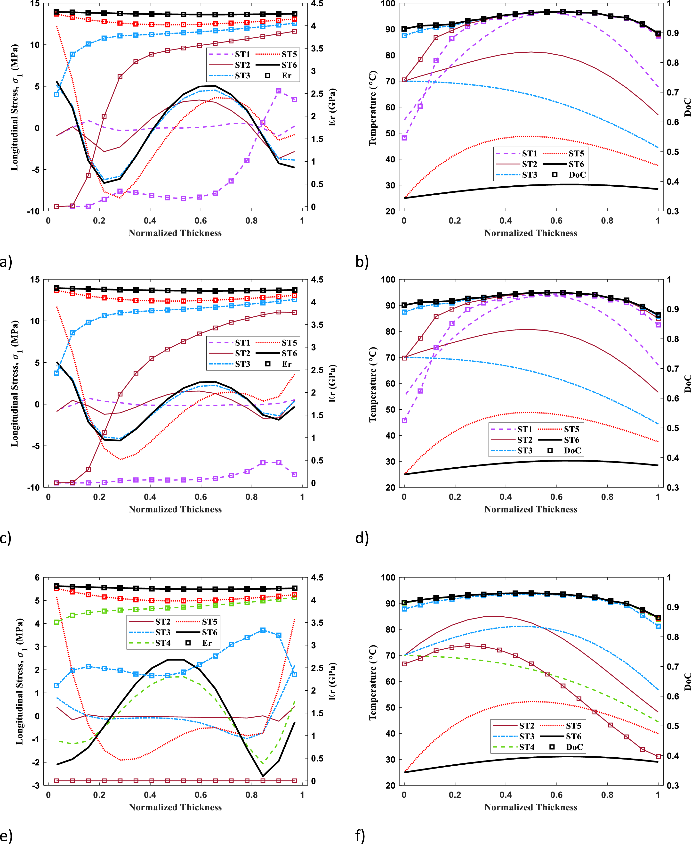

Despite the resin modulus being equal to $E_{r u b}$ at ST2 in Scenario 6, the significant magnitudes of resin modulus at ST1 for Scenarios 4 and 5 indicate that the curing process at TDLine occurs earlier in these two scenarios relative to Scenario 6 (see Figure 16(a), 16(c), 16(e)).

From ST1 to ST2, thermal expansion and chemical shrinkage are observed at the bottom of the TDLine (due to positive gradients of temperature and DoC in this region, see Figure 16(b) and 16(d), while thermal shrinkage occurs at the center and top of the TDLine (due to negative gradient of temperature here, see Figure 16(b) and 16(d). Due to the greater thermal shrinkage in the center region than in the top region and the higher resin modulus in the top region, the top region prevents the center region from shrinking freely. As a result, compressive stresses develop in the top region, while tensile stresses arise in the center region (see Figure 16(a) and 16(c)). As the position along the TDLine moves from the center region to the normalized thickness of about 0.2, thermal shrinkage decreases, leading to the development of compressive stress in this area. In the bottom region, chemical shrinkage predominates over thermal expansion, which would normally be expected to induce tensile stress. However, the development of tensile stress is negligible in this region because of the low resin modulus, which has not yet been developed tangibly. At ST2, the magnitudes of stresses for Scenario 4 are greater than those for Scenario 5 because of the higher resin modulus in Scenario 4 (see Figure 16(a) and 16(c)).

From ST2 to ST3, the region with a normalized thickness of around 0.6 experiences a greater thermal shrinkage relative to its neighboring regions (see Figure 16(b) and 16(d)), resulting in the development of tensile stress within this region and compressive stress in the adjacent regions. In the bottom region of TDLine, chemical shrinkage dominates, and simultaneously, resin modulus exhibits a significant increase (see Figure 16(a) and 16(c)). Therefore, tensile stress is developed within the bottom region, while compressive stress in the adjacent region is enhanced.

From ST3 to ST4 (not shown), the resin modulus increases in the bottom region. The bottom temperature remains constant at 70°C. Thermal shrinkage dominates in the center region, although with a small magnitude, resulting in insignificant residual stress development.

During the transition period from ST4 to ST5, the resin modulus increases in the bottom region. There is also a significant thermal shrinkage in this region (due to the negative gradient of temperature here, see Figure 16(b) and 16(d). With moving upward along the TDLine, thermal shrinkage gradually decreases, resulting in the development of tensile stress at the bottom and compressive stress at the center regions. Tensile stress also develops in the top region, which can be attributed to the need to fulfill the equilibrium condition (see Figure 16(a) and 16(c)).

During the transition from ST5 to ST6, thermal shrinkage predominates in the center region, resulting in the development of tensile stress in this region and compressive stress in the top and bottom regions. Although the longitudinal stress magnitudes at ST6 are lower for Scenario 5 than for Scenario 4 (due to earlier resin modulus development in Scenario 4), the qualitative longitudinal stress evolution during the curing process is similar for both scenarios (see Figure 16(a) and 16(c)).

The longitudinal residual stress evolution in Scenario 6 differs from Scenarios 4 and 5 due to differences in temperature and DoC distributions at the beginning of the curing stage (see Figure 16).

For Scenario 6, during the transition from ST2 to ST3, the resin modulus significantly increases along TDLine (see Figure 16(e)). Also, a chemical shrinkage occurs across TDLine with a dominant magnitude at the top region (see Figure 16(f)). Concurrently, thermal expansion is observed at the top region, while thermal shrinkage emerges in the bottom region (see Figure 16(f)). In the top region, chemical shrinkage predominates over thermal expansion (see Figure 16(f), compare DoC graphs for ST2 and ST3), resulting in the development of tensile stresses within the top region and compressive stresses in the neighboring region (see Figure 16(e), stress graph for ST3). The chemical shrinkage in the bottom region is higher compared to that in its neighboring region, leading to the development of tensile stress at the bottom of the laminate and compressive stress in the adjacent areas.

At a normalized thickness of approximately 0.2, the thermal shrinkage magnitude is greater than that in the bottom region (see Figure 16(f), compare temperature graphs for ST2 and ST3). This difference in thermal shrinkage leads to the development of tensile stresses in this region and compressive stresses in the neighboring areas. The state of stress in the TDLine is the result of the superposition of contributions from the aforementioned phenomena.

From ST3 to ST4 (Figure 16(e) and 16(f)), a complete through-thickness thermal shrinkage is observed, predominantly in the region with a normalized thickness of approximately 0.4. This shrinkage leads to the development of tensile stress in the center region and compressive stress in the top and bottom regions, respectively. Also, resin modulus develops throughout the TDLine during this phase of curing (Figure 16(e), compare Er graphs for ST3 and ST4), contributing to the observed stress levels. It is important to mention that the comparatively low stress levels observed during the initial phases of the curing stage can be primarily ascribed to the relatively low resin modulus at those points.

During the transition from ST4 to ST5, thermal shrinkage becomes dominant at the bottom region with a diminishing magnitude towards the top region (Figure 16(f), graphs for ST4 and ST5). However, chemical shrinkage is negligible along the TDLine. As a result, a high tensile stress appears in the bottom region, while around the center region, a high compressive stress arises. Tensile stress also develops in the top region to meet the equilibrium conditions, ensuring that the summation of longitudinal residual stresses along the TDLine remains zero.

From ST5 to ST6, thermal shrinkage dominates at the center region, leading to the development of tensile stress at the center region and compressive stress at the top and bottom areas.

As noted for thick laminates, longitudinal residual stresses may vary non-uniformly in both thickness and longitudinal directions.

Figure 17(a), 17(c), and 17(e) illustrate the temperature history and Tg evolution of the resin during the curing stage at the SPs a- e for Scenarios 4–6, respectively. In these figures, graphs with square markers represent Tg, while those without markers denote temperature. The corresponding resin modulus (Er) and longitudinal residual stress evolutions are presented in Figure 17(b), 17(d), and 17(f) for Scenarios 4, 5, and 6, respectively. In these figures, graphs with square markers represent Er, while those without markers represent longitudinal stress.

Figure 17.

Time histories of temperature and Tg for (a) Scenario 4, (c) Scenario 5, (e) Scenario 6 and time histories of longitudinal stress and resin modulus for (b) Scenario 4, (d) Scenario 5, and (f) Scenario 6 at sensing points (SPs) labeled as a-e during the curing stage.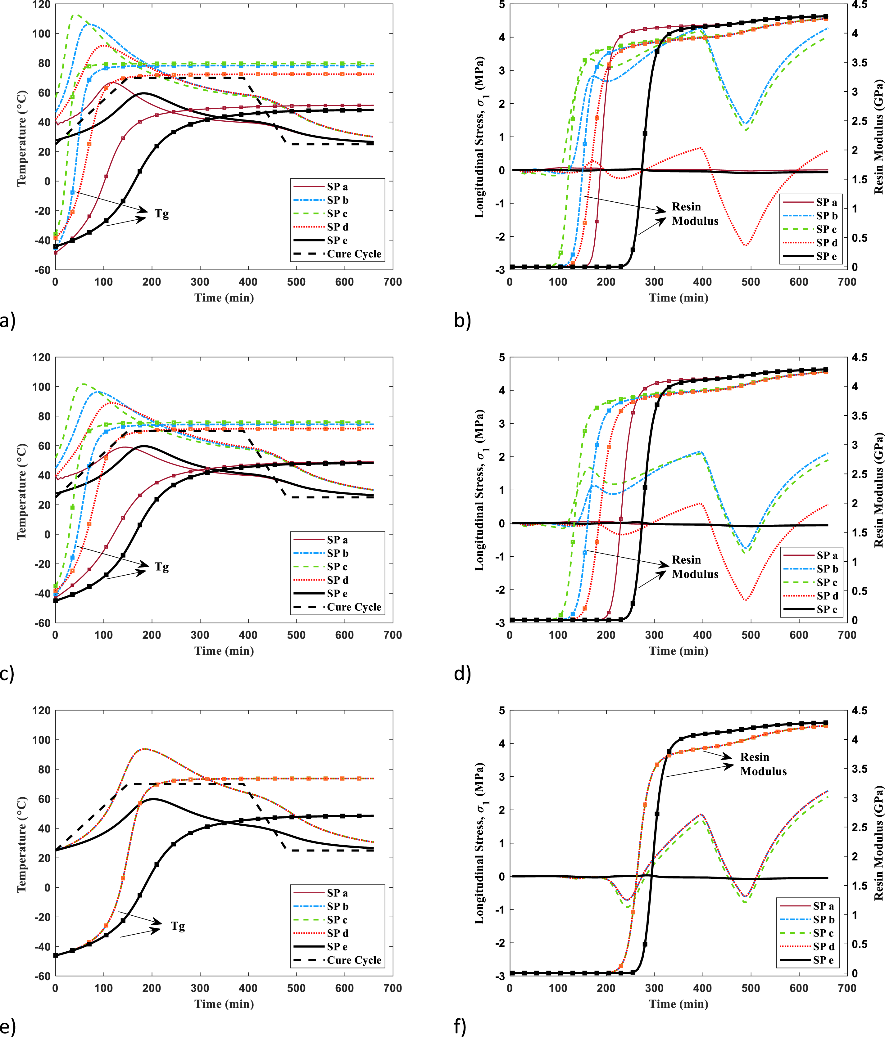

For Scenario 4 (Figure 17(a)), the maximum temperature recorded at SPs a, b, c, d, and e are 66.7°C, 106°C, 113°C, 91.7°C, and 59.5°C, respectively. The distinct temperature history graphs at SPs b, c, and d can be attributed to the variations in temperature and DoC magnitudes at the beginning of the curing process at these locations. Similar to the behavior observed in thick laminates, the resin modulus in ultra-thick laminates (Figure 17) starts to increase significantly at the mentioned SPs when the temperature difference between the glass transition temperature (Tg) and the actual temperature drops below approximately 25°C. First, the modulus enhancement is observed at SP c, followed by SP b, then SP d, SP a, and finally, SP e. Following the vitrification point, the continued increase in resin modulus can be attributed to the ongoing decrease in temperature. Vitrification (rubbery-to-glassy transition) occurred at SPs a-e at 241, 196, 158, 229, and 340 minutes, respectively.

The notable differences in longitudinal residual stress at SPs b, c, and d in the time range of 100 to 150 minutes can be primarily attributed to the disparities in resin modulus at these locations (Figure 17(b)). As a result of the earlier onset of resin modulus development at SP c compared to SP b, and at SP b compared to SP d, comparison of the magnitude of longitudinal residual stresses at these locations exhibits a decreasing trend. The highest stress magnitudes are observed at SP c, followed by SP b and SP d, respectively. The decrease and increase in longitudinal residual stresses at SPs b, c, and d in the time range of 150-270 minutes (ST2-ST3) reflect the competition between chemical shrinkage at the bottom region and thermal shrinkage at the center region. After ST2, the longitudinal residual stresses at SPs b, c, and d exhibit similar patterns of variation. For a more thorough examination of the mechanisms governing the longitudinal stress variations at SPs b, c, and d, the reader is encouraged to refer to the analysis of longitudinal stress variations along the thickness direction (TDLine) presented in the previous sub-section.

According to Figure 17(c), for Scenario 5, the maximum temperatures recorded at SPs a, b, c, d, and e are 59°C, 96.3°C, 101.6°C, 89°C, and 59.7°C, respectively. Vitrification took place at SPs a-e at times 296, 215, 180, 247, and 340 minutes, respectively. The lower maximum temperatures observed at SPs a, b, c, and d for Scenario 5 compared to Scenario 4 (see Figure 17(a) and 17(c) can be attributed to a lower initial maximum temperature and DoC values for Scenario 5 at the onset of the curing process (see Figure 7). Between the times of 100 and 200 minutes, the maximum longitudinal stress at SPs b, c, and d is higher for Scenario 4 compared to Scenario 5. This difference can be attributed to the earlier onset of resin modulus development at SPs b, c, and d in Scenario 4 as opposed to Scenario 5. The timing of modulus evolution directly impacts stress formation within the laminates. During the curing stage, the longitudinal stress evolution behavior observed for Scenario 5 follows a similar pattern as for Scenario 4 discussed earlier. At the end of the curing stage, the longitudinal stress magnitudes at SPs b and c for Scenario 4 are approximately twice that of Scenario 5 (see Figure 17(b) and 17(d)).

As shown in Figure 17(e) and 17(f), for Scenario 6, the temperature, Tg, and resin modulus histories at SPs b, c, and d are identical. This can be attributed to the initial uniform temperature and DoC fields at the beginning of the curing process, along with the positioning of the SPs away from the right and left edges. Furthermore, the temperature, Tg, resin modulus, and longitudinal residual stress histories at the edge SPs a and e are also identical, as depicted in Figure 17(e) and 17(f). The maximum temperatures recorded at SPs a and b are 59.8°C and 93.7°C, respectively. Vitrification also occurred at SPs a and b at times 315 and 357 minutes, respectively. The longitudinal stress history at SP c exhibits some differences when compared to the histories observed at SPs b and d. The observed difference can be attributed to the non-local nature of stress, which depends not only on the properties and conditions at a specific point but also on variations in the solution domain (refer to the corresponding stress contour plots in the coming pages).

Figure 18(a) and 18(b) present the resin modulus contour plots for Scenarios 4 and 5 at three selected curing times: 150 min (ST2), 270 min (ST3), and 390 min (ST4), respectively. For Scenario 6, the resin modulus is presented at the same STs except for ST2 since the resin modulus is not yet developed at this time. Therefore, resin modulus contour plot is presented at 230 min instead of at 150 min (ST2), as shown in Figure 18(c). To provide a more detailed visualization of the spatial distribution and temporal evolution of resin modulus within the ultra-thick laminates, the resin modulus contour plots are adjusted to exclude magnitudes below 0.1 GPa.

Figure 18.

Contour plots of resin modulus (Er) within the ultra-thick laminate at the times of 150 min (ST2), 270 min (ST3), and 390 min (ST4) for (a) Scenario 4, (b) Scenario 5, and (c) at the times of 230 min (after ST2), 270 min (ST3), and 390 min (ST4) for Scenario 6.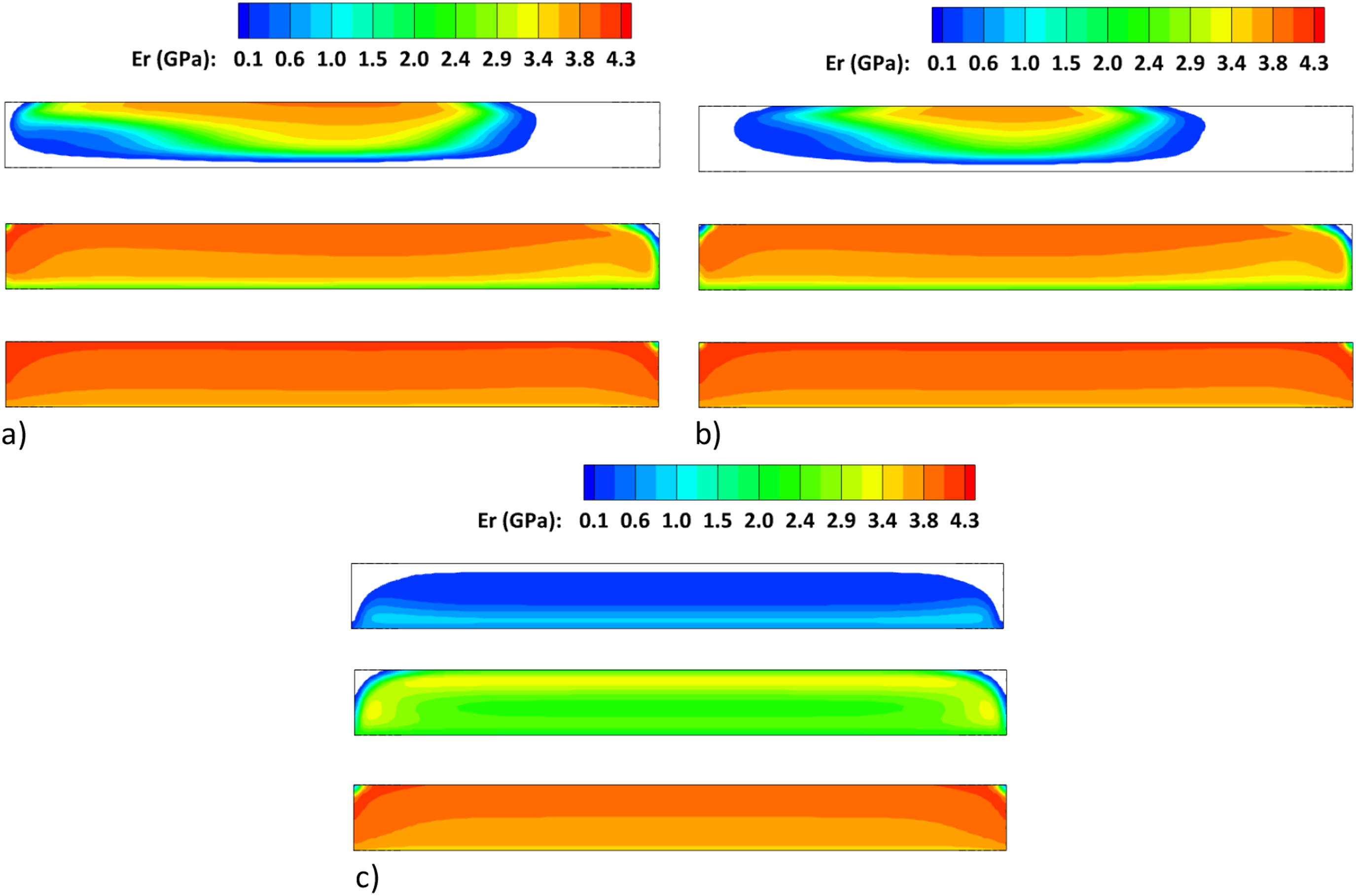

In Scenarios 4 and 5, resin modulus development begins at the top-center regions of the laminate. This early modulus evolution can be attributed to the elevated temperature and DoC levels within the laminates at the onset of the curing process (see Figure 7). In Scenario 6, the initial development of resin modulus is observed at the bottom of the laminate, which is in direct contact with the heat source. At ST3, the resin modulus remains undeveloped in the top-right corner of the laminate for all three scenarios, while the top-left corner exhibits different trends depending on the scenario. At the end of the process, the resin modulus distribution is homogeneous within the laminate for all three scenarios.

Figure 19(a) and 19(b) present longitudinal residual stress contour plots at five STs during the curing process (ST2 to ST6, from top to bottom) for Scenarios 4 and 5, respectively. While, for Scenario 6, Figure 19(c) presents the same stress at four STs (ST3, ST4, ST5, and ST6). This is because of the delay in the development of the resin modulus in Scenario 6 compared to the other two scenarios.

Figure 19.

Longitudinal residual stress contour plots within the ultra-thick laminate at different selected times (ST2 to ST6, from top to bottom) for (a) Scenarios 4, (b) Scenario 5, and (c) at different selected times (ST3 to ST6, from top to bottom) for Scenario 6.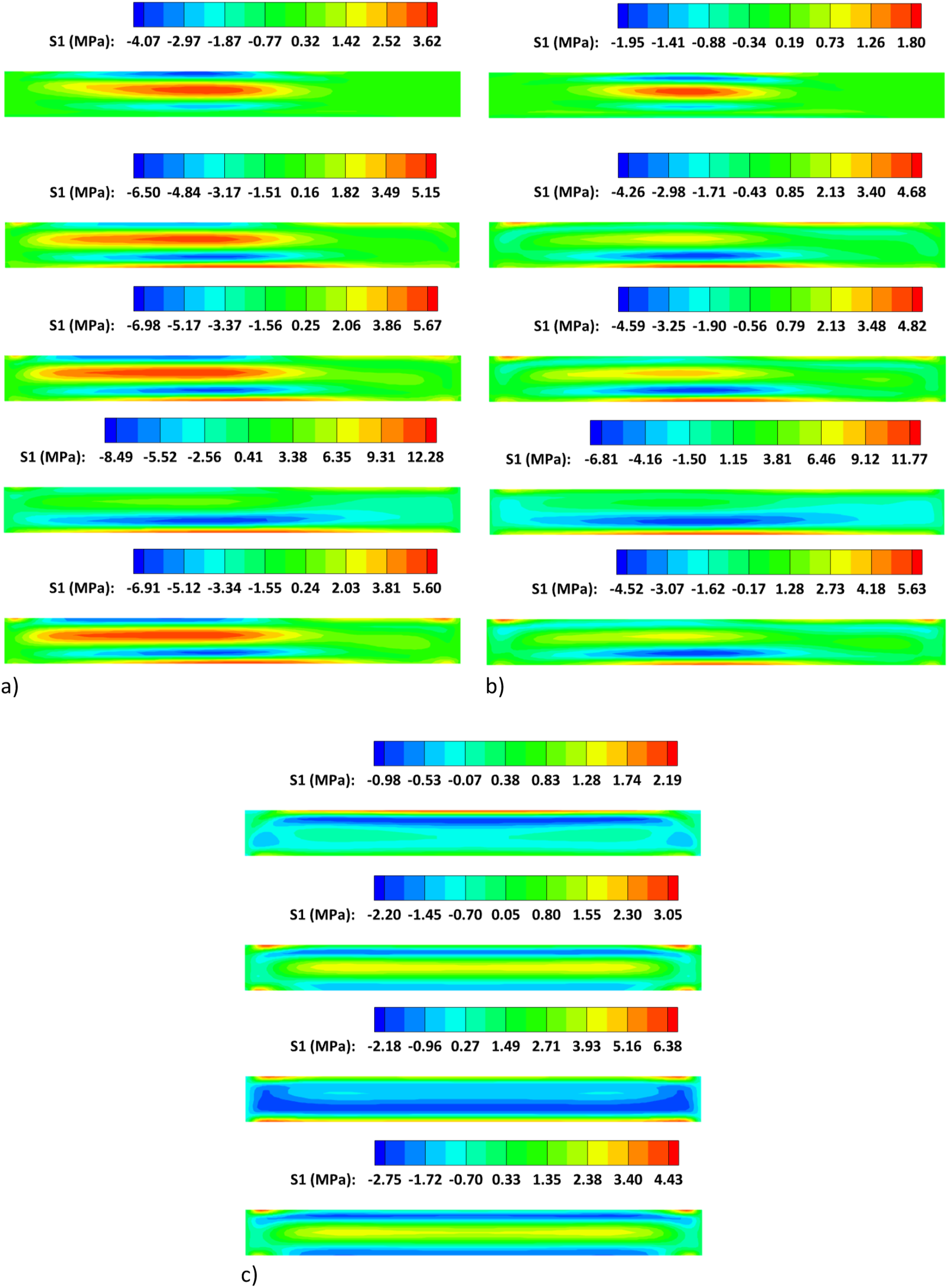

The stress contour plot for Scenarios 4 and 5 exhibits significant spatial variations along both the longitudinal and thickness directions. It seems the region, which has longitudinal stresses with significant magnitudes and variations along the thickness direction, corresponds to the region where resin modulus evolution is initiated from there (see Figure 18(a) and 18(b). Note that the longitudinal stress variations observed along the thickness direction at the mid-length of the laminate (TDLine) during the curing stage were previously discussed (see Figure 16). In contrast to Scenarios 4 and 5, Scenario 6 exhibits a more uniform variation of longitudinal residual stress along the longitudinal direction. During curing, maximum tensile/compressive longitudinal residual stresses are 12.28/8.49 MPa (Scenario 4), 11.77/6.81 MPa (Scenario 5), and 6.38/2.75 MPa (Scenario 6). Therefore, the maximum tensile and compressive longitudinal residual stress experienced within the ultra-thick laminate during the curing stage is associated with Scenario 4, in which the online resin mixing scheme is used.

At the end of the curing process, the maximum tensile/compressive longitudinal residual stress magnitudes (in MPa) observed in the laminate are 5.60/6.91 for Scenario 4, 5.63/4.52 for Scenario 5, and 4.43/2.75 for Scenario 6, respectively. Therefore, the maximum compressive longitudinal residual stress experienced within the ultra-thick laminate at the end of the curing stage is associated with Scenario 4, in which the online resin mixing scheme is used. Although there is a slight difference in tensile residual stress magnitudes when comparing Scenarios 4 and 5, it is worth noting that the maximum tensile residual stress value in Scenario 5 is 0.5% higher than that observed in Scenario 4.

Analysis of interlaminar normal residual stress evolution

Figure 20(a)–20(c) illustrate the distribution of interlaminar normal stress along the right edge (RE) and left edge (LE) of the laminate at ST2, ST3, ST4, ST5, and ST6 for Scenarios 4, 5, and 6, respectively.

Figure 20.

The interlaminar normal stress distributions at the right edge (RE) and left edge (LE) of the ultra-thick laminate at five selected times (ST2, ST3, ST4, ST5, and ST6) for (a) Scenario 4, (b) Scenario 5, (c) Scenario 6, and (d) the interlaminar normal stress distributions along LDLine for Scenarios 4, 5, and 6.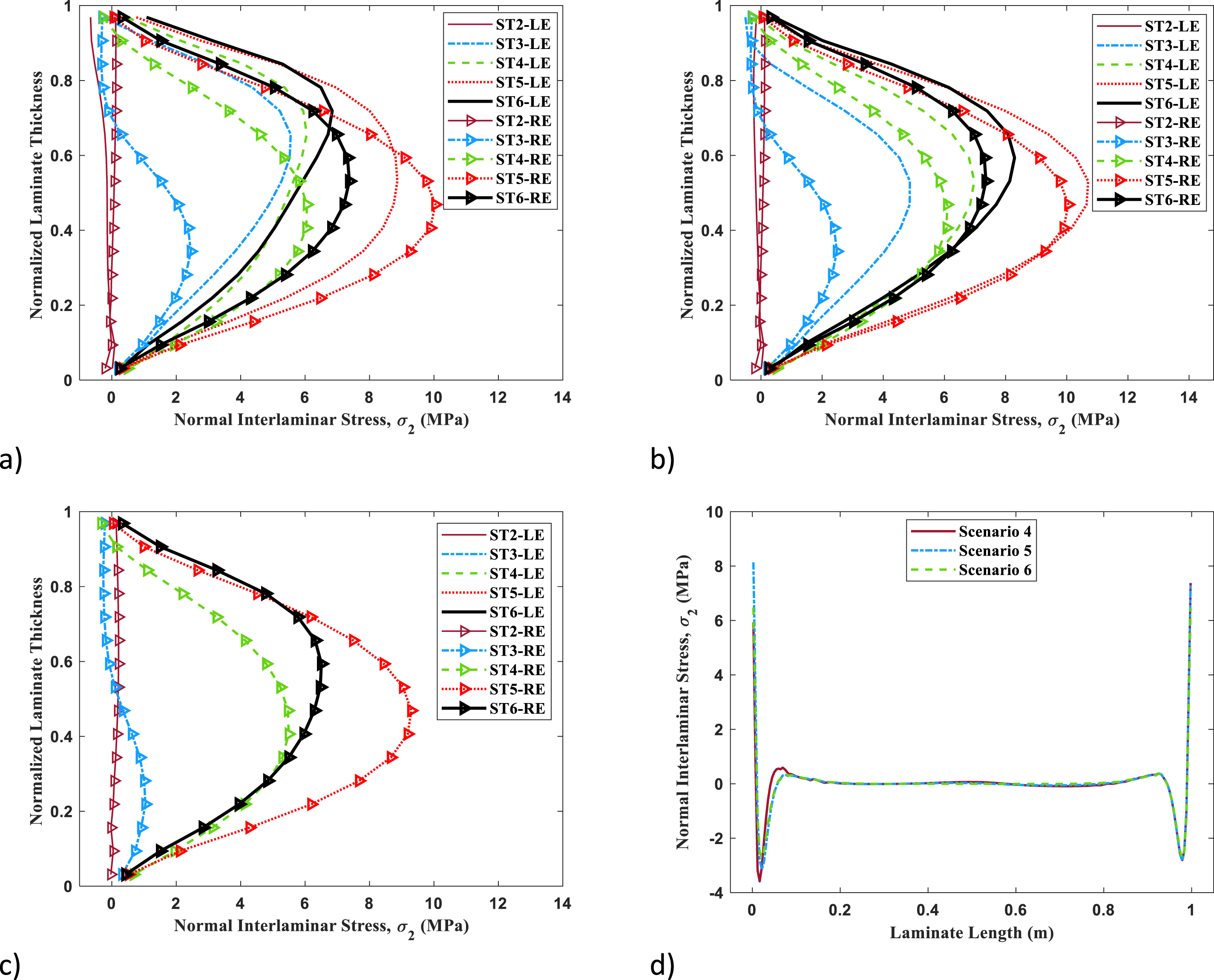

At the end of the curing stage, in the vicinity of the right and left edges of the ultra-thick laminates, the longitudinal stress at the top and bottom regions is tensile. Consequently, it was anticipated that the interlaminar normal stress would also be tensile at least at the top and bottom of these edges, as maintaining moment equilibrium about the out-of-plane axis at these regions of the laminate is required. To gain insight into the issue, it is helpful to isolate a rectangular element in the top-right of the laminate, considering its longitudinal and interlaminar normal stresses, and calculate the balance of moments at the bottom-left corner of the rectangular element. While compressive longitudinal stresses are present within the laminate away from the top and bottom regions, the tensile longitudinal stresses at the top and bottom regions are sufficiently strong to overcome the effect of compressive stresses. However, in order to maintain equilibrium of the longitudinal stresses, the laminate will experience a tensile interlaminar normal stress with a greater magnitude in its central regions.

For Scenario 6, the development of resin modulus and interlaminar normal stress at the right and left edges are the same (as shown in Figures 18(c) and 20(c), respectively). However, for Scenarios 4 and 5, resin modulus and normal interlaminar stress develop earlier at the left edge than at the right edge (see Figures 18(a), 18(b), 20(a), and 20(b)).

Based on Figure 20, at ST2, the interlaminar normal stress is negligible at the right edge of the laminate for all three scenarios due to the lack of resin modulus development in this region. For Scenarios 4 and 5, the early resin modulus development at the left edge, with magnitudes lower than 0.1 GPa (see Figure 18(a) and 18(b), results in the appearance of small compressive interlaminar stresses in this region. The compressive type of the interlaminar normal stress at the left edge in Scenarios 4 and 5 can be attributed to the presence of compressive longitudinal stress at the top of this edge. It is important to note that the type of interlaminar normal stress, whether tensile or compressive, along the right and left edges of the composite laminate is directly influenced by the magnitude and type of longitudinal residual stresses present near and along these edges.

At ST3, for Scenarios 4 and 5, the resin modulus exhibits some development throughout the right edge of the laminate, excluding the top corner region (Figure 18(a) and 18(b)). Therefore, a significant tensile interlaminar stress is developed in this area except at the top corner where a small compressive interlaminar stress as shown in Figure 20(a) and 20(b) happens. At the left edge of the laminates, the resin modulus has developed to a greater extent compared to the right edge. Therefore, the region where tensile interlaminar stress develops at the left edge is larger and experiences higher stress magnitudes than the corresponding region at the right edge. For Scenario 6, at the right and left edges, the observed development of resin modulus at ST3 is confined to the bottom half of the laminate (as illustrated in Figure 18(c)), which corresponds to the development of tensile and compressive interlaminar normal stresses in the bottom and top halves of the laminate, respectively.

At ST4, for Scenarios 4 and 5, the top region of the right edge exhibits a relatively lower magnitude of resin modulus compared to that of the left edge (see Figure 18(a) and 18(b)), which results in a lower magnitude tensile interlaminar normal stress at this region relative to the top region of the left edge, where the resin modulus is sufficiently developed. For Scenario 6, the low magnitudes of resin modulus observed at the top region result in a similar tensile interlaminar normal stress behavior to that observed at the right edge for Scenarios 4 and 5.

At ST5, the magnitude of longitudinal stresses in the laminate increases (see Figure 19(a) and 19(b), leading to an observed increase in the tensile interlaminar normal stress at both the right and left edges for Scenarios 4, 5, and 6 (see Figure 20). At ST5, tensile interlaminar stresses at the right and left edges of the laminate reach their peak values of 10 MPa (RE) and 8.5 MPa (LE) for Scenario 4, and 10 MPa (RE) and 11 MPa (LE) for Scenario 5. For Scenario 6, the maximum tensile stress is also 9.5 MPa for both right and left edges.

At ST6, tensile interlaminar normal stresses decrease as longitudinal stresses diminish (see Figure 19). Consequently, the maximum final interlaminar stresses at the right and left edges of the laminate are as follows: 7 MPa (RE) and 6.5 MPa (LE) for Scenario 4, 7 MPa (RE) and 8.5 MPa (LE) for Scenario 5, and 6 MPa for both edges in Scenario 6.

Comparing the results so far, the maximum interlaminar normal stresses observed during and at the end of the curing stage are attributed to Scenario 5, which are 11 MPa and 8.5 MPa, respectively.

In Scenario 4, the interlaminar normal stress distribution at the left edge displays skewness, with the maximum stress located closer to the top edge than its counterpart at the right edge (Figure 20(a)). This behavior can be attributed to the presence of the maximum DoC gradient in the thickness direction near the left edge of the laminate at the onset of the curing process (see Figure 7(b)). Additionally, resin modulus development initiates earlier at the left edge compared to the right edge in Scenarios 4 and 5 (Figures 17(b), 17(d), and 18(a), and 18(b)), while it coincides at both edges in Scenario 6 (Figures 17(f) and 18(c)). In Scenario 5, the presence of slight skewness in the interlaminar normal stress distribution at the left edge of the laminate along with higher stress magnitudes compared to the right edge, can be attributed to the high DoC gradient in the thickness direction near the left edge at the beginning of the curing process (see Figure 7(d)). Resin modulus development differences between the right and left edges further support this observation.

Figure 20(d) illustrates the interlaminar normal stress distribution along the LDLine of the laminate (see Figure 1) for Scenarios 4, 5, and 6. In each scenario, the tensile interlaminar normal stress at the ends of LDLine is accompanied by a significant compressive interlaminar normal stress to ensure the equilibrium is maintained.

Analysis of curing quality and process-induced deformation

Figure 21(a)–21(c) represent contour plots of DoC at the end of the curing stage for Scenarios 4, 5, and 6, respectively. The maximum DoC values for Scenarios 4, 5, and 6 exhibit values of 0.973, 0.957, and 0.947, respectively. The higher maximum DoC observed in scenario 4 compared to Scenario 5, and in Scenario 5 compared to Scenario 6, can be attributed to the higher temperatures experienced by the laminates for scenarios with higher maximum DoC (see Figure 17(b), 17(d), and 17(f), temperature history at SP c).

Figure 21.

Contour plots of DoC within the ultra-thick laminate at the end of the curing stage for (a) Scenarios 4, (b) Scenario 5, and (c) Scenario 6.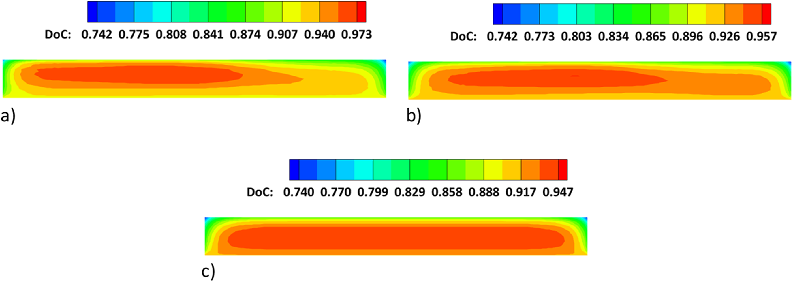

Notably, the maximum DoC values for Scenarios 4 and 5 are located in regions where resin gelation occurs first within the laminate. The more uniform DoC distribution observed in Scenario 6 compared to Scenarios 4 and 5 is attributed to the uniform temperature and DoC distributions considered at the onset of the curing stage (see Table 2).

The DoC values at the top corners of the laminates drop to a minimum of 0.74 (Figure 21), substantially lower than the value of 1 required for full resin curing. This indicates that the current cure cycle is inadequate for proper resin curing across the laminate thickness, especially in the top corners.

Figure 22(a)–22(c) depict the displacement component contour plots in the longitudinal (U1) and transverse (U2) directions on the deformed ultra-thick laminates at the end of the curing stage for Scenarios 4, 5, and 6, respectively. For clarity, laminate deformations in contour plots are exaggerated fivefold. It is essential to note that the presented deformations reflect the cumulative deformations from the onset of resin modulus enhancement until the end of the curing stage. For Scenarios 4 and 5, the resin modulus within the ultra-thick laminate begins to demonstrate a notable increase 80 minutes after the curing process has commenced (see Figure 17(b) and 17(d)). In contrast, Scenario 6 exhibits a significant enhancement in resin modulus starting from 200 minutes following the initiation of the curing stage (see Figure 17(f)).

Figure 22.

Contour plots of the displacement components (U1 and U2) on the deformed ultra-thick laminate at the end of the curing stage for (a) Scenarios 4, (b) Scenario 5, and (c) Scenario 6.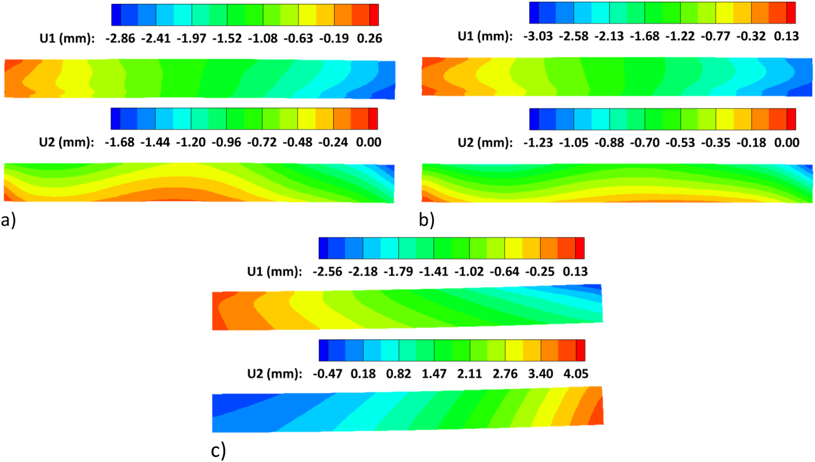

The displacement contour plots (U1 and U2) are similar for Scenarios 4 and 5, but differ from those in Scenario 6. In scenarios 4 and 5, the laminate exhibits a small downward deformation in the region near the right edge. Additionally, localized compressions in the thickness direction lead to localized thickness reduction in the laminate, as observed in the vertical displacement (U2) contour plots (Figure 22(a) and 22(b)). In Scenario 6, a prevalent upward deformation trend is observed in the longitudinal direction, with the magnitude of deformation escalating as the distance from the left edge increases (Figure 22(c)). Across all three scenarios, a degree of contraction in the longitudinal direction is observed. The maximum longitudinal displacement (U1) values recorded for Scenarios 4, 5, and 6 are −2.86 mm, −3.03 mm, and −2.56 mm, respectively, while the corresponding maximum vertical displacement (U2) values are −1.68 mm, −1.23 mm, and 4.05 mm. Therefore, the resin mixing scheme influences the deformation of ultra-thick laminates. However, considering non-uniform temperature and DoC distributions at the end of the bleeding stage as the initial conditions for the curing stage can alter the deformation type of the ultra-thick laminate. Essentially, this emphasizes the significance of taking these distributions into account, as they play a crucial role in shaping the residual stress development and deformation behavior throughout the curing process of ultra-thick laminates.

Thickness effect on simulation results of the curing stage

Table 4 provides an overview of the maximum longitudinal and interlaminar normal stresses observed both at the end and during the curing stage. Based on the results discussed so far, the maximum tensile and compressive longitudinal stresses observed at the end of the curing stage for the thick (50 mm) and ultra-thick (100 mm) laminates vary across the discussed scenarios, with maximum tensile stresses of 6.29 MPa (Scenario 1) and 5.63 MPa (Scenario 5) for the thick and ultra-thick laminates, respectively (see Table 4). Similarly, maximum compressive longitudinal stresses of 3.38 MPa (Scenario 1) and 6.91 MPa (Scenario 4) are observed for the thick and ultra-thick laminates, respectively. As Table 4 shows, the maximum residual tensile and compressive longitudinal stresses in the ultra-thick laminate are 10.5% lower and 104.4% higher relative to those in thick laminates, respectively, highlighting the influence of laminate thickness on the magnitude of residual stresses at the end of the curing process. Notably, the maximum tensile and compressive longitudinal residual stresses in thick and ultra-thick laminates are higher during the curing stage than those observed at the end. The maximum tensile and compressive longitudinal stresses observed during the curing stage for the thick (50 mm) and ultra-thick (100 mm) laminates also vary across the considered scenarios, with maximum tensile stresses of 8.47 MPa (Scenario 1) and 12.28 MPa (Scenario 4) for the thick and ultra-thick laminates, respectively (see Table 4). Similarly, maximum compressive longitudinal stresses of 4.62 MPa (Scenario 1) and 8.49 MPa (Scenario 4) are observed for the thick and ultra-thick laminates, respectively. During curing, ultra-thick laminates exhibit 45% higher tensile and 83.8% higher compressive longitudinal residual stresses than thick laminates. The maximum residual longitudinal stresses in thick and ultra-thick laminates do not exhibit a discernible trend across the different scenarios.

Table 4.

Summary of longitudinal and interlaminar normal stresses during and at the end of the curing stages.

		During curing stage			End of curing stage
		Thick	Ultra-thick	Diff. (%)	Thick	Ultra-thick	Diff. (%)
Longitudinal stress (MPa)	Max. Tensile	8.47 (Scen. 1)	12.28 (Scen. 4)	45	6.29 (Scen. 1)	5.63 (Scen. 5)	−10.5
Longitudinal stress (MPa)	Max. Compressive	4.62 (Scen. 1)	8.49 (Scen. 4)	83.8	3.38 (Scen. 1)	6.91 (Scen. 4)	104.4
Interlaminar Normal stress (MPa)	Max. Tensile	4.3 (Scen. 2)	11 (Scen. 5)	155.8	3.5 (Scen. 1)	8.5 (Scen. 5)	142.9

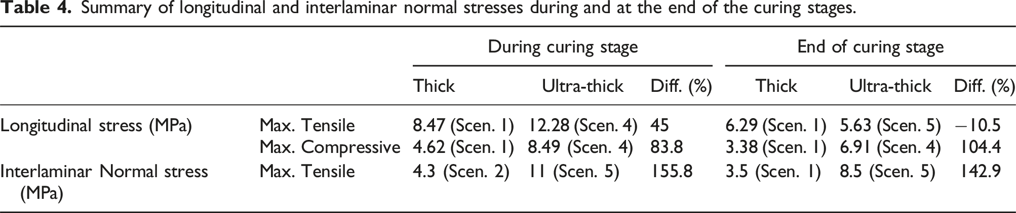
At the end of the curing stage, the maximum interlaminar normal stresses observed in the thick (50 mm) and ultra-thick (100 mm) laminates across different scenarios exhibit maximum values of 3.5 MPa (Scenario 1) and 8.5 MPa (Scenario 5), respectively, highlighting the significant impact of laminate thickness on the development of interlaminar normal residual stresses. Interestingly, the maximum interlaminar normal residual stress in the ultra-thick laminate is 142.9% higher than in the thick laminate. However, during the curing stage, the maximum interlaminar normal residual stresses experienced by the thick (50 mm) and ultra-thick (100 mm) laminates exhibit magnitudes of 4.3 MPa (Scenario 2) and 11 MPa (Scenario 5), which represent a 22.9% and 29.4% increase over the maximum interlaminar normal residual stresses observed at the end of the curing stage. These stresses occur at the left edges of the laminates, highlighting the influence of the resin mixing scheme on the development of these stresses.

For the ultra-thick (100 mm) laminates, the deformation behavior in Scenarios 4 and 5 differs from that in Scenario 6. The deformation behavior in Scenario 6 is similar to that of the thick laminates. The maximum vertical displacement observed in thick laminates is 4.1 mm (Scenario 3), while ultra-thick laminates exhibit a maximum vertical displacement of 10.6 mm (Scenario 6). Notably, these maximum displacements correspond to the scenarios where uniform temperature and DoC distributions are used at the onset of the curing stage. Increasing thickness and usage of non-uniform temperature and DoC distributions as initial conditions for the curing stage can lead to different deformation behaviors of laminates. Therefore, when conducting numerical simulations of ultra-thick laminates to determine their deformation behavior during the curing stage, it is essential to consider non-uniform temperature and DoC distributions (corresponding to the end of the bleeding stage) as initial conditions of the curing stage.

At the end of the curing stage, the ultra-thick laminates exhibit higher maximum DoC values (up to 0.973, see Figure 21) when compared to the thick laminates (up to 0.918, see Figure 14), attributable to the higher temperatures experienced within the ultra-thick laminates during the curing stage. The minimum DoC values observed at the top corners of both thick and ultra-thick laminates are as low as 0.74 (see Figures 14 and 21), well below the value of 1 required for complete resin curing. Thus, the current cure cycle is inadequate for full resin curing, especially in the top corners. To improve the DoC values and reduce residual stresses within ultra-thick laminates, it is necessary to investigate different curing strategies such as mold pre-heating and alternative cure cycles. Future research will prioritize the development and evaluation of alternative cure cycles that effectively address the critical issues of DoC, residual stress, deformations, and curing time in thick and ultra-thick laminates. This will include the identification and testing of various curing strategies to determine the most efficient and effective approach for these laminates.

Conclusion

This study has explored the development of longitudinal and interlaminar normal residual stresses within thick and ultra-thick laminates produced by the VI process, considering the underlying mechanisms that contribute to residual stress formation. In addition, the deformation of these laminates at the end of the curing stage was also investigated. Two different approaches were considered to study the influence of resin curing during the initial three stages (mold filling, flushing, and bleeding) of the VI process on the curing stage. The first approach uses a uniform DoC distribution within the laminates at the beginning of the curing stage, as calculated using the resin curing kinetic equation. This approach also considers the temperature distribution uniform and equal to the ambient temperature. In the second approach, the temperature and DoC distributions at the beginning of the curing stage were obtained using numerical simulation of the initial three stages of the VI process.

At the onset of the curing stage, the findings reveal that the maximum DoCs obtained through approach 2 (0.134 and 0.274) are 61.4% and 110.8% higher for thick (Scenario 1) and ultra-thick (Scenario 4) laminates, respectively, when compared to those obtained using approach 1 (0.083 and 0.13). Furthermore, approach 2 resulted in maximum temperatures of 39°C and 63°C for thick and ultra-thick laminates, respectively. Note that the uniform ambient temperature (25°C) was imposed on the laminate by approach 1. These results emphasize the substantial impact of the chosen approach on the DoC and temperature distributions within thick and ultra-thick laminates at the beginning of the curing stage.

A detailed examination of residual stress development in thick and ultra-thick laminates during the curing stage was conducted. The results revealed a substantial discrepancy between the maximum tensile and compressive longitudinal residual stresses in ultra-thick laminates when compared to their thick laminate counterparts. Furthermore, the distribution of longitudinal residual stresses in the thickness direction for thick and ultra-thick laminates was found to differ significantly. Upon completion of the curing stage, it was observed that the maximum interlaminar normal stress at the left edge of the ultra-thick laminate was 143% greater than that of the thick laminate. This substantial difference underscores the significant impact of laminate thickness on the magnitudes of interlaminar normal stress at the edges of laminates.

The type of resin mixing can affect the magnitudes of longitudinal and interlaminar normal residual stresses at the end of the curing stage. However, the influence of resin mixing type was more significant in ultra-thick laminates than thick laminates.

At the end of the curing stage, it was observed that the maximum vertical displacements for thick laminates were 10.62 mm and 5.69 mm for Scenarios 3 and 1, respectively. These displacements correspond to the utilization of approaches 1 and 2, respectively, highlighting the influence of the applied approach on the deformation behavior of the thick laminates under investigation. In the case of ultra-thick laminates, the maximum vertical displacements were found to be 4.05 mm for Scenario 6 and -1.68 mm for Scenario 4, corresponding to the application of approaches 1 and 2, respectively. The application of approach 2 led to a change in the deformation behavior of the ultra-thick laminate. These findings confirm that accurate deformation prediction requires simulating resin curing effects during initial VI stages. Therefore, when the primary objective is to numerically predict deformations of the thick and ultra-thick laminates, it is crucial to incorporate a comprehensive simulation of the resin curing phenomena occurring in the three initial stages of the VI process (approach 2) for reliable and accurate results.

At the end of the curing stage, the DoC magnitudes varied from 0.74 to 0.918 and 0.74 to 0.973 for thick and ultra-thick laminates, respectively. This indicates that the currently used cure cycle (MRCC) is not suitable for curing thick and ultra-thick laminates, as these DoC magnitudes deviate significantly from the expected values of 1 for complete cure. To improve the DoC values, reduce residual stresses, and minimize curing time in thick and ultra-thick laminates, it is crucial to explore alternative cure cycles that achieve uniform DoC distribution and adequate resin curing throughout the laminate. This will involve investigating different curing strategies, including mold pre-heating, to identify the most effective cure cycle for thick and ultra-thick laminates. Developing and evaluating such alternative cure cycles will be an important focus of future work to address these issues. Another important point to be examined in future work is the influence of tool-part interaction on residual stress evolution within thick and ultra-thick laminates.

Footnotes

Acknowledgments

The authors would like to express their gratitude for the financial support.

Declaration of conflicting interests

The author(s) declared no potential conflicts of interest with respect to the research, authorship, and/or publication of this article.

Funding

The author(s) disclosed receipt of the following financial support for the research, authorship, and/or publication of this article: This research was partially funded by the Iran National Science Foundation (INSF) through grant number 98001017.

ORCID iDs

Mostafa Nasiri

Ali Abedian

Data Availability Statement

The data that support the findings of this study are available from the corresponding author, upon reasonable request.*

References

Struzziero

Teuwen

JJE

. Effect of convection coefficient and thickness on optimal cure cycles for the manufacturing of wind turbine components using VARTM. Compos Appl Sci Manuf 2019; 123: 25–36.

Ruiz

Trochu

. Numerical analysis of cure temperature and internal stresses in thin and thick RTM parts. Compos Appl Sci Manuf 2005; 36(6): 806–826.

Chava

Namilae

. Continuous evolution of processing induced residual stresses in composites: an in-situ approach. Compos Appl Sci Manuf 2021; 145: 106368.

Liu

Zheng

Gao

, et al. Comparative study on the effect of cure parameters on residual deformation for thermoset composite laminates. J Compos Mater 2021; 55(19): 2591–2604.

Kim

H-S

Yoo

S-H

Chang

S-H

. In situ monitoring of the strain evolution and curing reaction of composite laminates to reduce the thermal residual stress using FBG sensor and dielectrometry. Compos B Eng 2013; 44(1): 446–452.

Sorrentino

Esposito

Bellini

. A new methodology to evaluate the influence of curing overheating on the mechanical properties of thick FRP laminates. Compos B Eng 2017; 109: 187–196.

Bogetti

Gillespie

. Process-induced stress and deformation in thick-section thermoset composite laminates. J Compos Mater 1992; 26(5): 626–660.

Ding

Fang

, et al. Experimental and numerical investigation of tool-part interaction on the process-induced distortions in composite structures. Compos Struct 2022; 279: 114871.

Yuan

Wang

Peng

, et al. An analytical model on through-thickness stresses and warpage of composite laminates due to tool–part interaction. Compos B Eng 2016; 91: 408–413.

10.

Lahuerta

Nijssen

van der Meer

, et al. The influence of curing cycle and through thickness variability of properties in thick laminates. J Compos Mater 2017; 51(4): 563–575.

11.

Zhou

Cheng

, et al. Quantitative relations between curing processes and local properties within thick composites based on simulation and machine learning. Mater Des 2023; 226: 111686.

12.

Cao

Pavier

, et al. Investigation of non-uniform gelation effects on residual stresses of thick laminates based on tailed FBG sensor. Compos Struct 2018; 202: 1361–1372.

13.

Ruiz

Trochu

. Multi-criteria thermal optimization in liquid composite molding to reduce processing stresses and cycle time. Compos Appl Sci Manuf 2006; 37(6): 913–924.

14.

Zhang

Hui

, et al. A multi-dwell temperature profile design for the cure of thick CFRP composite laminates. Int J Adv Manuf Technol 2021; 117(3): 1133–1146.

15.

Struzziero

Teuwen

JJE

. A fully coupled thermo-mechanical analysis for the minimisation of spring-in and process time in ultra-thick components for wind turbine blades. Compos Appl Sci Manuf 2020; 139: 106105.

16.

Athreya

Mehta

, et al. Numerical modeling and experimental validation of nonisothermal resin infusion and cure processes in large composites. J Reinforc Plast Compos 2017; 36(10): 780–794.

17.

Nasiri

Abedian

. Influence of resin curing during mold filling on process-induced residual stresses and deformations in ultra-thick vacuum-infused laminates: a multiphysics approach. Polym Compos.

18.

Zhang

Liu

Zheng

, et al. A fast spatio-temporal temperature predictor for vacuum assisted resin infusion molding process based on deep machine learning modeling. J Intell Manuf 2024; 35(4): 1737–1764.

19.

Siddig

Denis

Comas-Cardona

, et al. Infusion and polymerization of thick glass/Elium® acrylic thermoplastic resin composites. In: ICCM23. Belfast: ICCM, 2023.

20.

Chen

. An integrated flow-curing model for predicting residual stresses in textile composites. In: Mechanical Engineering. University of Connecticut, 2019.

21.

Yang

Liu

Jia

, et al. Coupled filling-curing simulation and optimized design of cure cycle in liquid composite molding. Int J Adv Manuf Technol 2024; 132(5): 2489–2501.

22.

Shojaei

Reza Ghaffarian

Mohammad Hossein Karimian

. Three-dimensional process cycle simulation of composite parts manufactured by resin transfer molding. Compos Struct 2004; 65(3): 381–390.

23.

Tan

Pillai

. Numerical simulation of reactive flow in liquid composite molding using flux-corrected transport (FCT) based finite element/control volume (FE/CV) method. Int J Heat Mass Tran 2010; 53(9): 2256–2271.

24.

Gupta

Kelly

. Optimal galerkin finite element methods for non-isothermal liquid composite moulding process simulations. Int J Heat Mass Tran 2013; 64: 609–622.

25.

Yalcinkaya

Caglar

Sozer

. Effect of permeability characterization at different boundary and flow conditions on vacuum infusion process modeling. J Reinforc Plast Compos 2017; 36(7): 491–504.

26.

Robinson

. Simulation of the vacuum assisted resin transfer molding (VARTM) process and the development of light-weight composite bridging. UC San Diego, 2008.

27.

Yong

Aktas

May

, et al. Out-of-plane permeability measurement for reinforcement textiles: a benchmark exercise. Compos Appl Sci Manuf 2021; 148: 106480.

28.

Barcenas

Narayana

Khoun

, et al. Thermochemical and rheological characterization of highly reactive thermoset resins for liquid moulding. J Compos Mater 2023; 57(19): 3013–3024.

29.

Pascault

Williams

RJJ

. Relationships between glass transition temperature and conversion. Polym Bull 1990; 24(1): 115–121.

30.

Struzziero

Nardi

Sinke

, et al. Cure-induced residual stresses for warpage reduction in thermoset laminates. J Compos Mater 2020; 54(22): 3055–3065.

31.

Mesogitis

Skordos

Long

. Stochastic simulation of the influence of fibre path variability on the formation of residual stress and shape distortion. Polym Compos 2017; 38(12): 2642–2652.

32.

Bejan

Poterasu

. Woven composite material design by orthotropic compliance averaging method using mathematica. Comput Methods Appl Mech Eng 1999; 179(1): 53–65.

33.

Zobeiry

Forghani

, et al. Multiscale characterization and representation of composite materials during processing. Philos Trans A Math Phys Eng Sci 2016; 374: 20150278.

34.

Danzi

Schneeberger

Ermanni

. A model for the time-dependent compaction response of woven fiber textiles. Compos Appl Sci Manuf 2018; 105: 180–188.

35.

Yenilmez

Caglar

Sozer

. Viscoelastic modeling of fiber preform compaction in vacuum infusion process. J Compos Mater 2017; 51(30): 4189–4203.

36.

Kim

White

. Viscoelastic analysis of processing-induced residual stresses in thick composite laminates. Mech Adv Mater Struct 1997; 4(4): 361–387.

37.

Herakovich

. Mechanics of fibrous composites. 1st ed. Wiley, 1997.