
Abstract
Sample selection models, variants of which are the Heckman and Heckit models, are increasingly used by political scientists to accommodate data in which censoring of the dependent variable raises concerns of sample selectivity bias. Beyond demonstrating several pitfalls in the calculation of marginal effects and associated levels of statistical significance derived from these models, we argue that many of the empirical questions addressed by political scientists would – for both substantive and statistical reasons – be more appropriately addressed using an alternative but closely related procedure referred to as the two-part model (2 PM). Aside from being simple to estimate, one key advantage of the 2 PM is its less onerous identification requirements. Specifically, the model does not require the specification of so-called exclusion restrictions, variables that are included in the selection equation of the Heckit model but omitted from the outcome equation. Moreover, we argue that the interpretation of the marginal effects from the 2 PM, which are in terms of actual outcomes, are more appropriate for the questions typically addressed by political scientists than the potential outcomes ascribed to the Heckit results. Drawing on data from the Correlates of War database, we present an empirical analysis of conflict intensity illustrating that the choice between the sample selection model and 2 PM can bear fundamentally on the conclusions drawn.
Introduction
Empirical research in political science has increasingly used Heckman’s sample selection model to accommodate datasets in which censoring of the dependent variable raises concerns of biases emerging from sample selectivity. Recent examples include the study by Lebovic (2004) of the influence of democracy on the contribution to peacekeeping operations, the analysis by Drury et al. (2005) of the amount of US disaster relief assistance, and the analysis by Böhmelt (2010) of the effectiveness of third-party intervention in conflict mediation. All of these studies observe the outcome of interest – in these examples various forms of foreign aid – only when it is positive, with the remainder of observations censored at zero. This raises the possibility that the sample used for estimation is non-random, in turn causing bias through the correlation of the error term with the explanatory variables. Heckman (1979) developed a two-stage estimator, alternatively called the Heckit or sample selection model, to mitigate this bias. In stage one, referred to as the selection equation, a probit model is estimated on the entire dataset to capture the determinants of censoring. Stage two, referred to as the outcome equation, involves estimation of a heteroskedasticity-corrected OLS regression on the non-censored observations. To control for potential bias emerging from sample selectivity, this second stage regression appends the inverse Mills ratio calculated from the probit model as an additional regressor.
While the Heckit model is extensively documented and can be readily implemented with standard statistical packages, its application is predicated on a particular conceptualization of the data generation process whose implications for estimation and interpretation often go unheeded by applied researchers. Among the first questions to resolve when modeling censored data is whether the censored observations represent missing values or whether they are more appropriately treated as zeros (Dow & Norton, 2003). With respect to the modeling of foreign aid, for example, a missing value would indicate that there is some latent level of foreign aid that is unobservable to the analyst, while a zero value would indicate that the level of foreign aid is just that, zero. This distinction has far-reaching implications for both the type of model applied to the data and the conclusions drawn from it.
The Heckit model treats censored observations as missing, which gives rise to the sample selection problem that the model is designed to correct. Results are typically interpreted in terms of potential outcomes; that is, the coefficient estimates measure the effect of an explanatory variable on foreign aid levels, irrespective of whether foreign aid is, in fact, expended. Were the censored values of the dependent variable instead regarded as zeros and hence observable, there would be no sample selection problem to address, though the analyst would still be confronted with the challenge of how to model a dependent variable populated with a large share of zeros.
One technique for handling such a data pattern is the two-part model (2 PM). Like the Heckit, this model involves the estimation of a probit and OLS regression, but is distinguished by the omission of the inverse Mills ratio from the latter regression. Results from the 2 PM are interpreted in terms of actual outcomes, with the coefficients measuring the effect of an explanatory variable on the actual amount of foreign aid expended.
The purpose of the present article is to undertake a comparative analysis of the Heckit and two-part models, highlighting the conditions under which each should be used as well as some of the pitfalls in their interpretation, particularly as regards the calculation of marginal effects and associated levels of statistical significance. Our central thesis is that many of the empirical questions addressed by political scientists using the Heckit model would – for both substantive and statistical reasons – be more appropriately addressed using a 2 PM, though we are aware of no instances in the political science literature where the 2 PM has been applied. We regard this neglect as a missed opportunity for three reasons.
First, a strong case can be made that the actual outcomes obtained from the 2 PM provide a tighter conceptual fit to the analytical objectives pursued by a wide range of political science studies, including investigations of federal domestic outlays (Jeydel & Taylor, 2003), military conflict (Koch & Gartner, 2005; Peterson & Graham, 2011), arms exports (Blanton, 2005), foreign direct investment (Jensen, 2003), and refugee flows (Moore & Shellman, 2006). Second, while it is never possible to identify the true data generation process, several methodological studies summarized in Puhani (2000) point to the superiority of the 2 PM over the Heckit based on Monte Carlo evidence.
Third, the 2 PM has less onerous identification requirements. In particular, it absolves the modeler of the need to specify so-called exclusion restrictions, variables that are included in the selection equation of the Heckit model but omitted from the outcome equation. In the absence of such variables, the functional form of the model provides the sole basis for its identification, which, if not achieved, can potentially result in biases that are more severe than the selection bias itself (Brandt & Schneider, 2007). Many – if not most – applied studies in political science that use the Heckit model disregard this important issue entirely.
The following section of the article takes a closer look at the structural differences between the Heckit and two-part models, including the derivation of their marginal effects as well as a brief discussion of statistical inference. Thereafter, we present an empirical example illustrating how the conclusions drawn from an analysis may be substantially altered depending on whether the censored values of the dependent variables are modeled as missing values or zeros. This example uses data compiled by Sweeney (2003) from the Correlates of War (COW) database to analyze the incidence and intensity of interstate conflict. The penultimate section provides guidance on the choice between the models, and the final section of the article concludes.
Two-part and Heckit models
For many years the Tobit model was among the most frequently applied tools in political science research for addressing data with a large share of zeros. In a highly influential article, Sigelman & Zeng (1999) called this practice into question, noting several restrictive features of the Tobit and illustrating the use of the Heckman model as an often superior alternative. As discussed in Wooldridge (2010) and others (e.g. Lin & Schmidt, 1984), among these restrictions is the Tobit model’s assumption that any variable which increases the probability of a non-zero value must also increase the mean of positive values. Quoting at length from Maddala (1992), Sigelman & Zeng (1999) additionally make what they deem to be an elementary – if not routinely neglected – point that the Tobit model is only appropriate in cases where the dependent variable can, in principle, take on negative values. They list several studies from the literature that use a Tobit model on a dependent variable for which the idea of negative values is indeed questionable, including analyses of PAC contributions to congressional candidates and the use of force in foreign policy.
Although Sigelman & Zeng (1999) provide useful insights into the proper use and interpretation of the Heckman model, their analysis leaves out some important aspects, most notably the correct calculation of statistical significance and questions relating to model identification. In what follows, we attempt to augment their work by filling in these gaps and by illustrating the advantages of including the two-part model in the practitioner’s toolkit.
Overview of the models
To accommodate missing or zero values of a dependent variable, two-stage estimation procedures can be employed, such as the sample selection model by Heckman (1979) or the two-part model, the latter of which was developed by Cragg (1971) as an extension to the Tobit model. Both types of models order observations of the outcome variable y into two regimes. The first stage defines a dichotomous variable R, indicating the regime into which the observation falls:
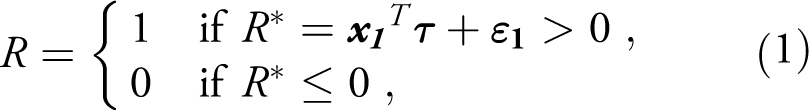
where
After estimating τ using Probit estimation methods, the second stage of both models involves estimating the parameters β via an OLS regression conditional on R = 1, i. e. y > 0:
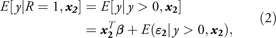
where
The prediction of the dependent variable consists of two parts, with the first part resulting from the first stage (1),
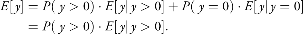
In the 2 PM, where it is assumed that

As Wooldridge (2010: 697) notes, the 2 PM assumes that both parts of the model are independent conditional on the observed characteristics
In this regard, a key distinguishing feature between the 2 PM and the Heckit model is that the second stage OLS regression of the latter is based on a conditional expectation that includes the inverse Mill’s ratio as an additional regressor to control for sample selectivity:
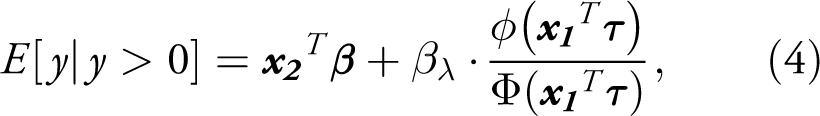
where
Model identification
In contrast to the 2 PM, one of the critical steps in specifying the Heckit model is the selection of exclusion restrictions, variables included in
Within the field of political science, Sartori (2003) is one of the few authors to take on the issue of identification directly when she develops an estimator for binary outcome selection models that does not require exclusion restrictions. In this respect, her model is similar to the 2 PM, though it is tailored to the specific case in which both the selection variables and the outcome variables are binary. Brandt & Schneider (2007) undertake an analysis that includes the case in which a selection model is used with a continuous outcome variable. Noting the extreme sensitivity of the results to the identification of the selection process, the conclusion they draw from a Monte Carlo analysis echoes that of earlier studies: that the cure afforded by the selection model may be worse than the disease.
This message has yet to find resonance in the applied literature, perhaps owing in part to the perception that the selection model and its companion, the Tobit model, are still the best options when dealing with censored data. Based on a review of over 20 articles from political science journals that used the Heckit model, listed in Table I, we were hard-pressed to find instances in which exclusion restrictions, identification, and/or associated problems with multicollinearity and bias receive even passing mention. Although several studies specify variables in x 1 that could potentially be regarded as exclusion restrictions, virtually none – with the notable exceptions of Shrestha & Feiock (2011) and Karreth & Tir (2013) – provide a theoretical justification that elaborates why these variables are hypothesized to uniquely determine the selection process but not the outcome variable. Likewise, having invoked selection bias as the justification for employing the Heckit model, the common practice is to subsequently ignore this issue in the discussion of the results, with no interpretation ascribed to the coefficients on the exclusion restrictions in the selection equation and an often erroneous interpretation ascribed to the magnitude and statistical significance of the coefficients in the outcome equation. Moreover, none of the articles listed in the table specify the basic question of whether the potential or actual outcomes are of interest.
Interpretation and statistical inference
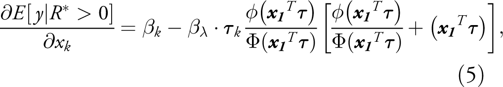
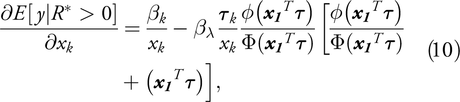
For both the Heckit and 2 PM, part of the challenge in this respect is in extracting quantities of substantive interest from the model coefficients. Noting the widespread misinterpretation of results from the Heckit model, Sigelman & Zeng (1999) demonstrate that the marginal effects of the variables that appear in both the selection and outcome equations are generally not given by the coefficient estimates, themselves, but rather must be calculated by differentiating Equation (4). This differentiation yields a unique conditional marginal effect for every observation in the data:
where
In their discussion, Sigelman & Zeng (1999) omit the precise interpretation of Equation (5), which is that of a potential outcome. This interpretation is relevant when the aim is to measure the effect of an explanatory variable for all observations in the data, including those for which the dependent variable is unobserved. For example, in research on wages – perhaps the most widespread application of the model – the concern is typically with quantifying the influence of attributes such as schooling on the potential wage of all working-age individuals, irrespective of whether the individual is in fact employed. But whether the notion of potential outcomes is equally apt for issues such as foreign aid, the use of military force or arms exports seems more questionable. With respect to arms exports, for example, the question arises as to whether interest really centers on modeling the latent expected value of arms exports that might have occurred under different circumstances for countries that export no arms, or on the actual observed level of exports for countries that do export arms.
Political science applications of the sample selection model
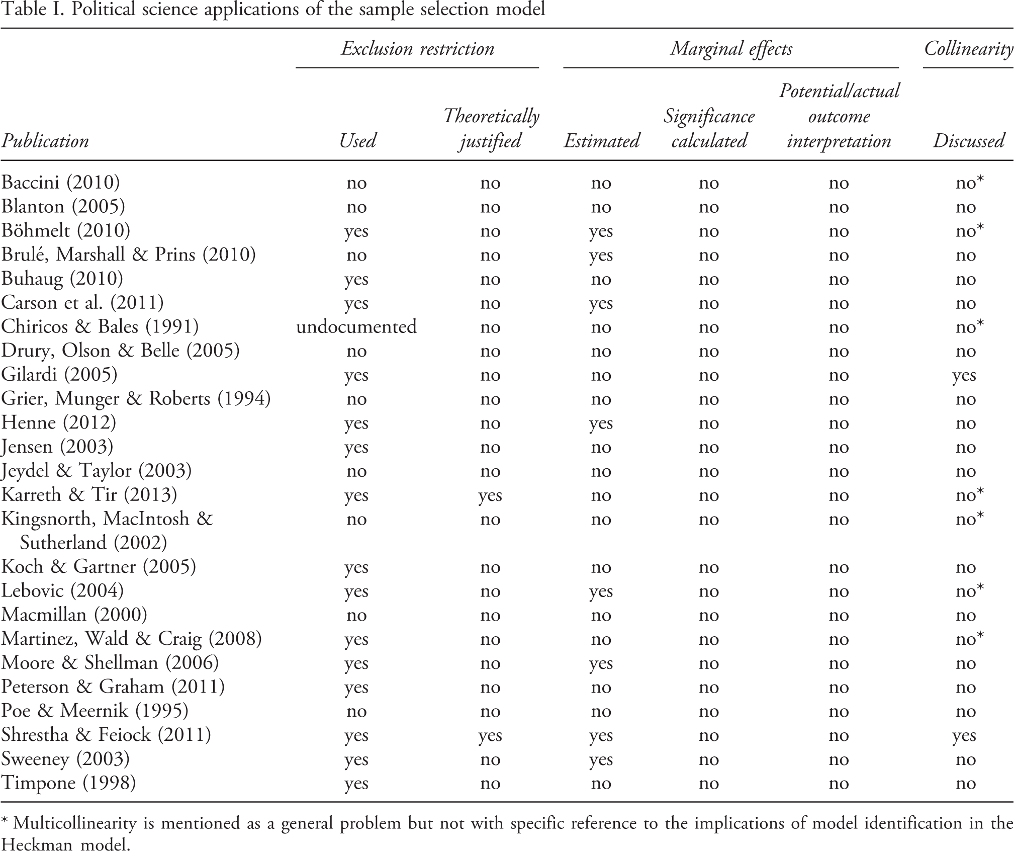
* Multicollinearity is mentioned as a general problem but not with specific reference to the implications of model identification in the Heckman model.
As Dow & Norton (2003) show, the Heckman model can also be used to retrieve such an actual outcome, with the marginal effect given by: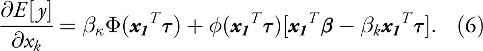
In practice, however, the Heckit model is rarely used for this purpose, perhaps owing in part to the need to select exclusion restrictions for the first stage of the model. As Duan et al. (1984) have argued, another reason is that the 2 PM typically has a lower mean square error than the Heckit when analyzing actual outcomes.
The marginal effect corresponding to the actual outcome from the 2 PM is likewise observation-specific and given by the differentiation of Equation (3):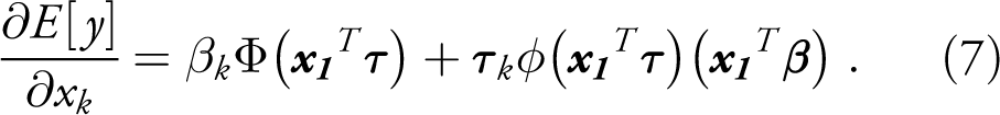
It bears emphasizing that the formulae (6) and (7) are only valid for the particular case in which the dependent variable and the explanatory variable of interest are continuous and are measured in levels; they are not valid for logged variables, dummies, or other functional forms. This point appears to be often overlooked in applications to political data, though it can have a major bearing on the estimate. If the variable is a dummy, for example, it instead makes sense to take the difference in the expected value function when x is set at 1 and 0, thereby capturing the discrete change in y. Presuming interest is on the potential outcome, the marginal effects of dummies in the Heckit model would then be calculated as: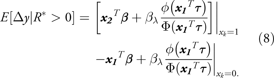
The marginal effect for dummies in the 2 PM, corresponding to the actual outcome, is: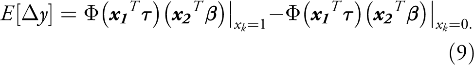
Other formulas would be required for cases in which the dependent variable, explanatory variable, or both are in logs, one of which is illustrated in the next section. In general, these formulas involve taking the partial derivatives of the expected values with respect to the variable of interest. As illustrated by Frondel & Vance (2012), somewhat more involved formulae are required for calculating the marginal effects of interaction terms, requiring the calculation of the second derivative,
An additional complication in interpreting the marginal effects from the Heckit and 2 PM relates to the calculation of their statistical significance. Because the formulae for the marginal effects are non-linear and comprised of multiple parameters, calculation of their standard errors is typically too complex to undertake analytically. Consequently, most studies abstain from assessing the statistical precision of the marginal effect estimates. As a work-around to this difficulty, Sigelman & Zeng (1999) suggest assessing the sensitivity of the estimate by referencing its standard deviation as well as its minimum and maximum values, a recommendation taken up by Sweeney (2003) and Brulé, Marshall & Prins (2010). Although the spread of the marginal effect is of interest in its own right, the drawback of this approach is that it cannot be used to test the hypothesis that the estimate is statistically significant. Indeed, a marginal effect estimated over a tight range of values may well be statistically insignificant and vice versa; what matters is the precision with which the underlying parameters are estimated.
Various methods exist for quantifying this precision, one of which is the delta method, which involves using a Taylor series to create a linear approximation of a non-linear function for computing the variance. An alternative is to bootstrap the standard errors. Both approaches, which are described in more detail in Vance (2009), can be readily implemented using most statistical software and yield an estimate of the standard error corresponding to the marginal effect of each observation in the data. In lieu of these procedures, many authors implicitly assume that the significance levels obtained on the coefficients carry over to the marginal effects and draw inferences accordingly. As demonstrated from the application of the delta method in the following section, this approach is ill-advised: the statistical significance level of the coefficient estimates provides no indication of the precision with which the marginal effects are estimated.
An empirical example
To illustrate the practical implications of the above issues, we undertake a comparative analysis of Heckman’s sample selection model and the 2 PM by drawing on the study of conflict severity by Sweeney (2003). This analysis is primarily concerned with the effects of military capability, interest similarity, and their interaction as causes of conflict severity among dyads. To test the significance of these determinants, the author estimates the maximum likelihood variant of the selection model, conventionally referred to as the Heckman model, using data from the Correlates of War militarized interstate dispute dataset, from which he derives a severity of dispute measure suggested by Diehl & Goertz (2000) for use as the dependent variable. This variable is censored at zero for cases in which the dispute severity is – using the logic of the Heckman model – not sufficiently intense to be observable; otherwise it assumes some positive value as calculated by a weighted combination of factors, including fatalities and the level of hostility.
The first column of Table II presents the coefficient estimates from the selection equation applied in both the Heckman and 2 PM. Column 2 presents the coefficients from the outcome equation of the Heckman model, which are identical to those presented as Model 1 in Sweeney’s original article, and column 3 contains the coefficient estimates from the outcome equation of the 2 PM. While the discussion that follows will focus primarily on the marginal effects derived from the estimates in columns 2 and 3, we note for now that the magnitude of most of the coefficient estimates are similar. One exception is the coefficient on the dummy variable Contiguous, whose magnitude and precision is considerably higher in the 2 PM, reaching statistical significance at the 1% level. Also of note is the statistical insignificance of the coefficient on the IMR, which would suggest rejecting the Heckit model in favor of the 2 PM. 1
Sample selection and two-part models of dyadic dispute onset and severity, 1886–1992
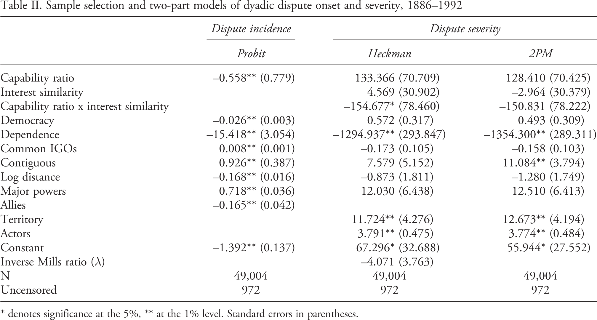
* denotes significance at the 5%, ** at the 1% level. Standard errors in parentheses.
Heckman results revisited
Sweeney focuses attention primarily on the first three variables in the outcome equation of Table II, a logged measure of the military capability of the states in the dyad (Capability ratio), a measure of their interest similarity (Interest similarity), and the interaction of the two. Additional controls are included for the democratization of the dyad (Democracy), its bilateral trade (Dependence), common membership in intergovernmental organizations (Common IGOs), a dummy indicating whether the states are contiguous (Contiguous), the logged distance between them in thousands of kilometers (Log distance), and dummies indicating whether the dyad is comprised of major powers (Major powers), whether the dyad members are allies (Allies), and whether the dispute is over territory (Territory). The model also includes a measure of the number of actors involved in the dispute (Actors).
While the question of model identification via exclusion restrictions is not taken up in the article, the dummy variable Allies is presumably intended to serve this purpose, being included as a determinant of conflict incidence but excluded as a determinant of conflict intensity. Whether a theoretical case for this choice can be made is questionable. Of the 972 observations on positive conflict intensity observed in the data, 251, about 25%, took place among dyads classified as allies. It is plausible that this attribute would not only affect the probability of conflict, but also its intensity, rendering it an inappropriate variable for identifying the model.
Table III presents select marginal effects derived from the model. Columns 1 and 2 present Sweeney’s derivation of the mean marginal effects averaged over the observations – all of which are calculated using Equation (5) – and their associated standard deviation, respectively. Column 3 presents an updated calculation of the mean marginal effect that takes into account the functional form of the explanatory variables (continuous, dummy, logged, or interacted) and column 4 presents the associated standard error, calculated using the delta method.
Mean marginal effect estimates
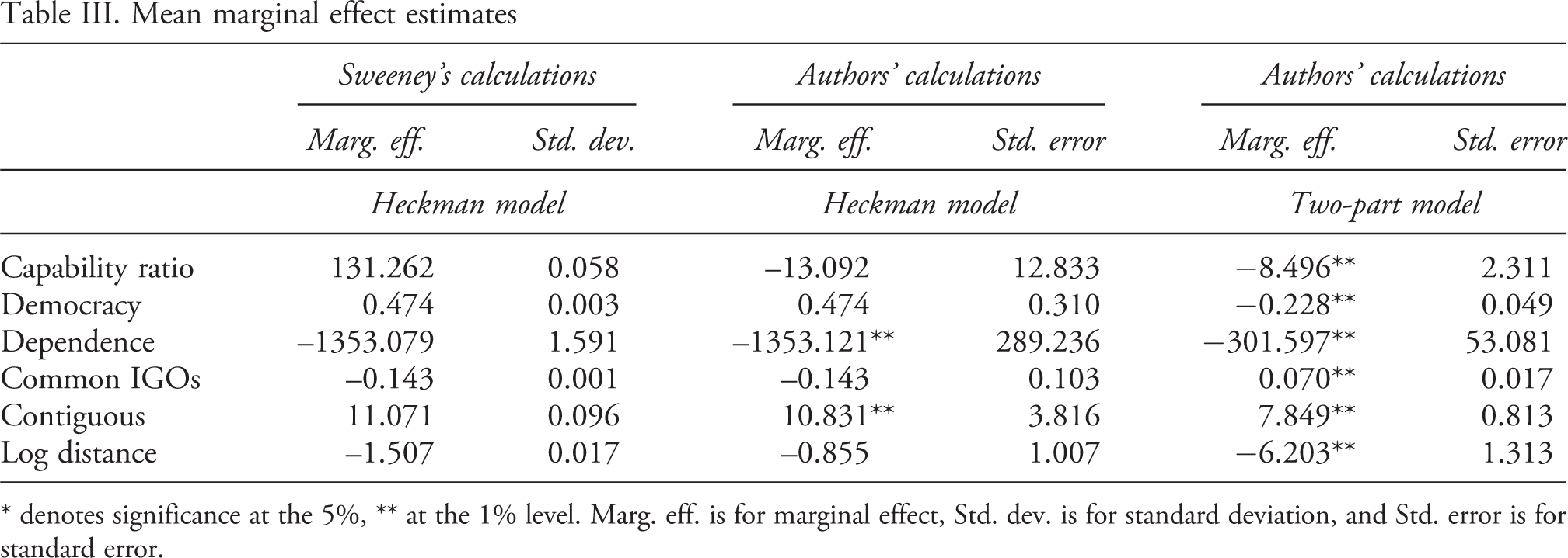
* denotes significance at the 5%, ** at the 1% level. Marg. eff. is for marginal effect, Std. dev. is for standard deviation, and Std. error is for standard error.
An even sharper discrepancy is seen for the variable Capability ratio, the variable of primary interest in the original study, which is both logged and interacted with the variable Interest similarity in the outcome equation. The marginal effect for this variable is given by:
where
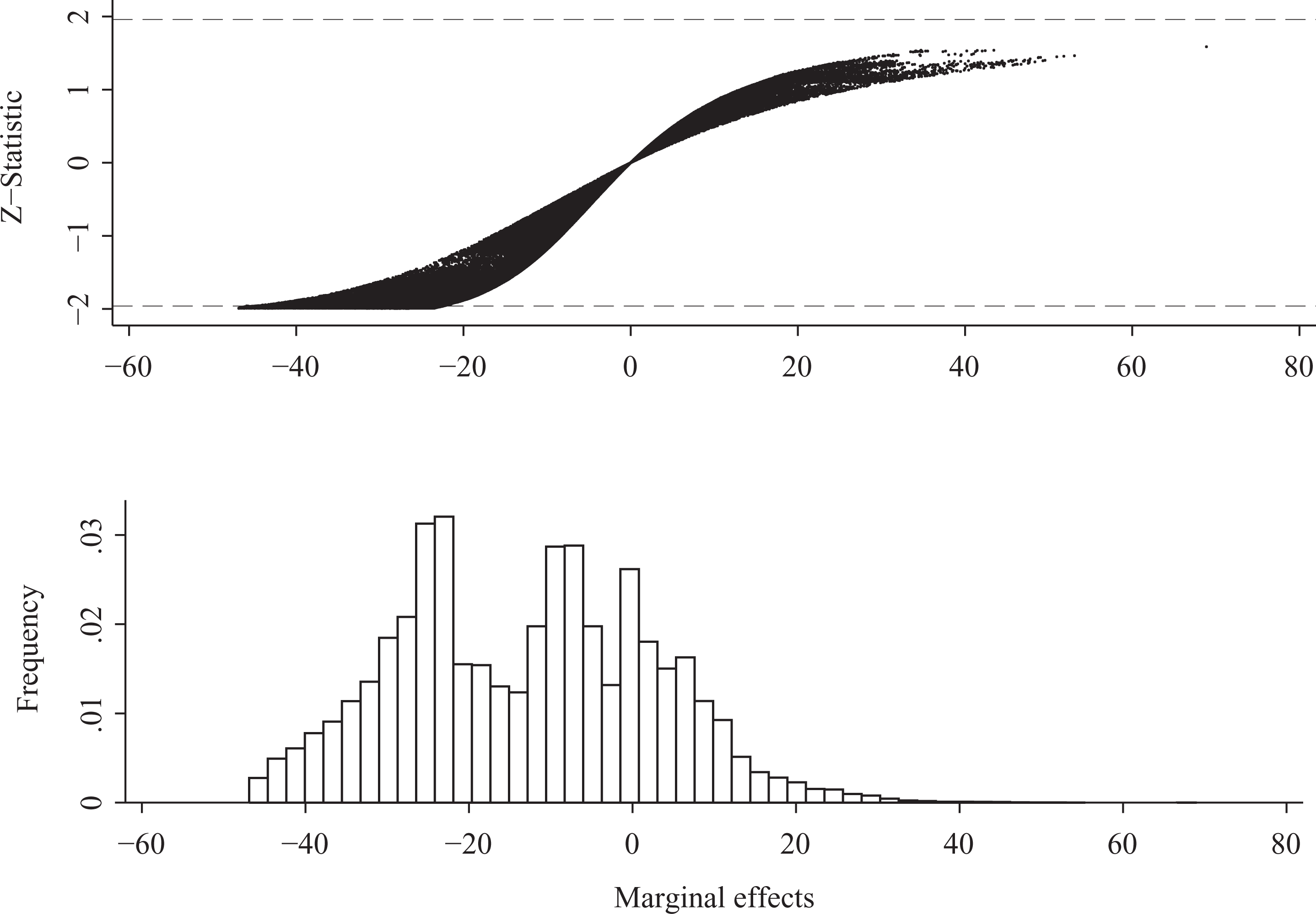
Further insight into the effect of the Capability ratio can be gleaned from plotting each observation-specific marginal effect against its associated z-statistic. The top panel of Figure 1 presents this plot for the whole range of observations. Relatively few points fall outside the absolute 1.96 threshold that indicates significance at the 5% level, and all of these have a marginal effect less than or equal to –25. The majority of marginal effects estimates – including all of those with a positive sign – are statistically insignificant. The histogram in Panel 2 facilitates a more transparent view of the distribution of marginal effects that shows the density corresponding to each value; three peaks in the density are visible at values of around –25, –8, and 0. This pattern highlights how in non-linear models the individual marginal effects can vary significantly depending upon at what point in the data the effects are calculated. Overall, the impression conveyed by Figure 1 is markedly different from the seemingly tightly estimated mean of 131.26 (with a standard deviation of 0.058) in column 1 of Table III.
In this regard, it bears noting that the standard deviations describing the spread of the marginal effects in column 2 are not remotely related to the statistical significance of these effects. Nor is it possible to infer the significance level of the marginal effects by referencing the standard errors in Table II. For example, the coefficient of the Contiguous dummy in Table II is statistically insignificant, leading Sweeney (2003: 746) to discard its importance, even though its marginal effect is significant at the 1% level. The opposite pattern is seen for the variable Democracy: its coefficient is statistically significant at the 10% level while the marginal effect is insignificant.
Two-part results
The final two columns of Table III present the marginal effects and standard errors derived from the 2 PM. The marginal effects of continuous level variables and of dummies are derived from Equations (7) and (9), respectively. The formula for logged variables is given by
Marginal effects of capability ratio from the Heckman model
If the logged variable is additionally interacted with a levels variable, as in the case of the interaction of the Capability Ratio with Interest Similarity, then the formula is given by:
Several notable differences are revealed by a comparison of the 2 PM and Heckman results, both with respect to the magnitude and sign of the marginal effects and their statistical significance. For example, while the magnitude of the mean estimate on the Capability Ratio from the 2 PM is, at –8.5, roughly 35% lower than that of the Heckman model, its precision is considerably higher. Figure 2 plots the observation-specific marginal effects against the Z-statistic. The plot is limited to the 920 uncensored observations on warring dyads, in line with the 2PM’s focus on actual outcomes. Statistically significant results are obtained over most of the observations in the data. Moreover, with the exception of a single observation, all of the estimated results fall below zero. Thus, contrasting with Sweeney (2003), this finding lends support to the hypothesis that dyads characterized by a preponderance of power of one of the states have less intense conflicts.
Two other contrasting results pertain to the variables Democracy and Common IGOs. The marginal effects of these variables are positive and negative, respectively, in the Heckman model, though neither is statistically significant. Conversely, they have the opposite signs and are highly significant in the 2 PM. Specifically, the results suggest that each unit increase in the democracy index is associated with a 0.22 decrease in conflict intensity among warring dyads, providing some confirmation to the argument that democracies are more peaceful vis-à-vis each other. By contrast, each unit increase in the index of membership in intergovernmental organizations is associated with a 0.017 increase in conflict intensity. While at first blush counter-intuitive, this may reflect the tendency for states to seek membership in IGOs on the basis of interests for which they have a large stake, with a corresponding willingness to wage war.
Which model to use?
The foregoing comparison brings into sharp relief why careful reflection surrounding selection of the appropriate model is warranted; the results and conclusions drawn from the analysis may depend fundamentally on this choice. Unfortunately, there are no hard and fast rules that point to the superiority of one model over the other in any given situation. As Madden (2008) has suggested, it therefore behooves researchers to consider a combination of criteria – theoretical, practical, and statistical – for guiding model selection.
With respect to theoretical considerations, the most important issue to resolve is whether the goal of the study is to model potential or actual outcomes, along with the related question of whether the censored observations on the dependent variable constitute Marginal effects of capability ratio from the 2 PM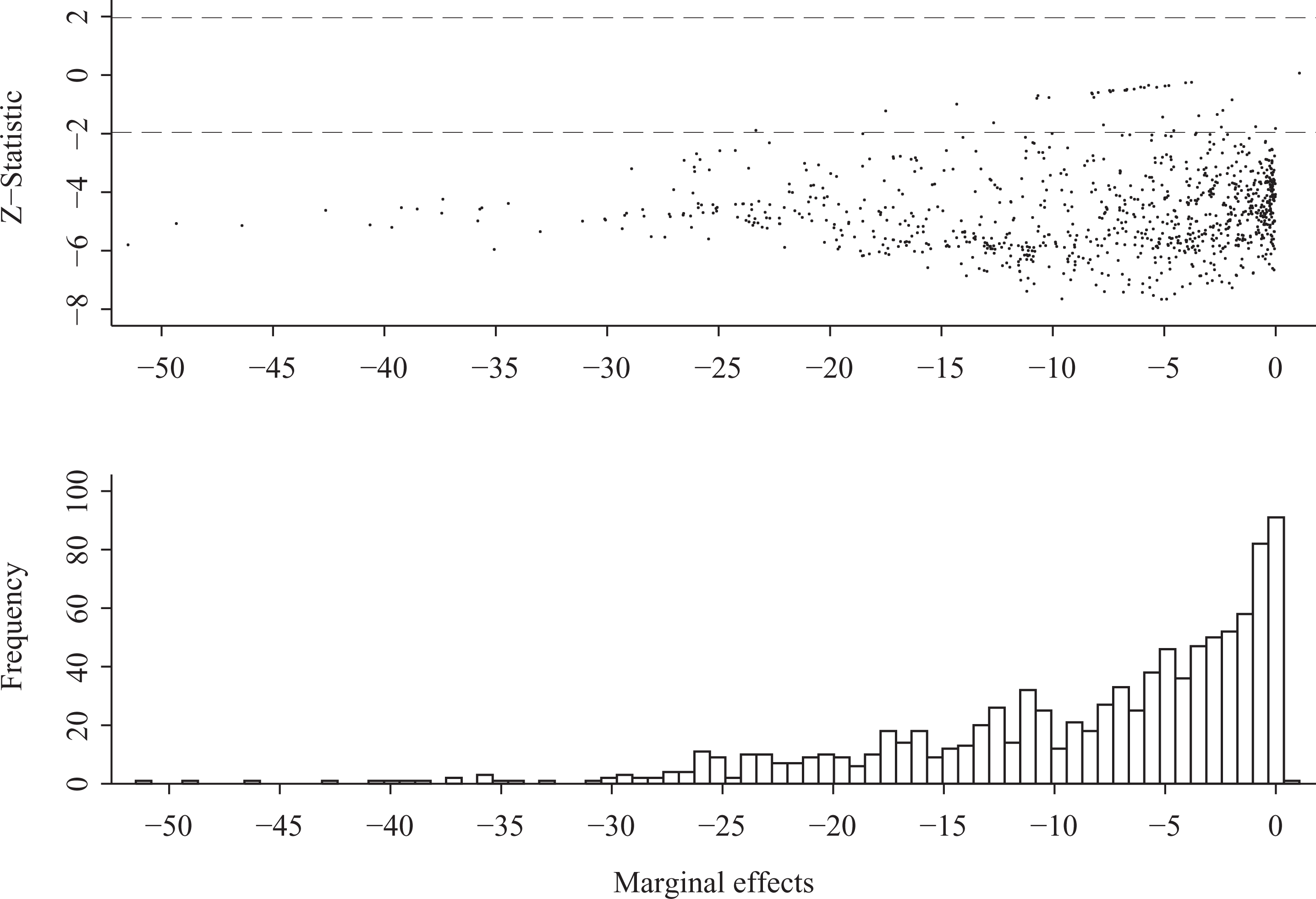
Nevertheless, we speculate that many political science applications using data with a large share of zeros aim to model actual outcomes, even when this objective is not stated explicitly. In one recent example, Carson et al. (2011) estimate a Heckman model to analyze the determinants of whether political challengers run for office in US Congressional races and, given so, the share of the vote they win in the election. The outcome equation of the model thus examines ‘election results once experienced candidates have made their entry decisions’ (Carson et al., 2011: 472). This phrasing, as well as the subsequent interpretation of the results in terms of the challengers who actually run for office (at the exclusion of those who might have run), suggests that the authors are primarily concerned with the actual outcomes of elections rather than the outcomes that might have occurred for those who did not run.
Presuming that the actual outcome is of interest, then the Heckman model, coupled with Equation (6) to recover the corresponding marginal effects, may still be the appropriate choice. Whether this is the case will depend on additional statistical and practical considerations. The balance would tilt toward application of a Heckman model if: (1) the analyst has reservations about the 2PM’s assumption that the discrete and continuous parts of the model are independent conditional on
Even when theoretically supported exclusion restrictions can be identified and a statistically significant coefficient on the inverse Mills coefficient points to the application of a Heckman model, caution is warranted. Wooldridge (2010) presents an example of an a Exponential Type II Tobit, of which the Heckit model is one variety, yielding an implausibly signed yet highly significant estimate of the selectivity parameter along with other difficult-to-interpret results, leading him to conclude that the ‘model has some serious shortcomings even if we accept the exclusion restrictions’ (Wooldridge, 2010: 702). Based on results from a Monte Carlo example, Dow & Norton (2003) also urge caution. Their simulations show that when there is a high degree of correlation between a coefficient and the inverse Mills coefficient, the magnitude of the former may be unusually small and that of the latter unusually high, biasing the results of a t-test on the inverse Mills ratio in favor of the Heckman model in exactly those models in which the t-statistic on a coefficient of interest is unusually small.
It is therefore imperative to undertake statistical diagnostic tests to assess the extent to which multicollinearity may afflict the results. One such diagnostic is afforded by the condition number, among several suggested by Belsley (1991) for assessing the extent of multicollinearity. This measure, which indicates how close a data matrix
Conclusion
Censored data is a prevalent feature of political science research, one that has been increasingly addressed by applying Heckman’s sample selection model. The purpose of the present article has been to cast a critical light on how this empirical approach is commonly implemented in the applied literature. Using the Heckman analysis of conflict intensity by Sweeney (2003), we pointed out several pitfalls in the derivation of marginal effects and their statistical significance. Our estimates, which took into account the functional form of the explanatory variable of interest, suggested fundamentally different conclusions than those reached by Sweeney concerning the impact of key variables in the model. Beyond this, we pursued the more basic issue of the selection model’s applicability to the questions typically addressed by political scientists, and suggested that a closely related alternative, the two-part model, may afford a more appropriate means for modeling the data generation process.
Whether this is the case hinges on whether the aim of the analysis is to model potential or actual outcomes. Potential outcomes are of relevance when the modeler treats the censored values as unobserved and wants to estimate the effect of an independent variable for both these and the observed realizations of the dependent variable. Sample selection bias may emerge in this case if there are unobserved variables that determine both selection into the sample and the outcome variable. To correct for this bias requires the specification of theoretically supported exclusion restrictions in the selection equation of the model, a critical step that is often disregarded in applied work.
When the aim is to instead model actual outcomes – that is, the effect of an independent variable on positive values of the dependent variable – sample selection bias is not of relevance because the censored values of the dependent variable are observed and treated as zeros. We believe this case is far more prevalent in political science data. Foreign aid was cited as one of several examples of a fully observed dependent variable for which the notion of missing values is inappropriate: the absence of foreign aid plausibly represents a case in which zero foreign aid is expended, just as the absence of conflict, refugee flows, arms sales, or foreign direct investment plausibly represents instances in which each of these dependent variables is zero. This interpretation suggests the application of the two-part model. One of the key practical advantages of the model is that no exclusion restrictions are required for its identification, making it less sensitive to specification errors.
Instances may nevertheless arise when the choice between the models is unclear. When this occurs, we would advocate estimating both models to explore the extent to which the results diverge. If the divergence is found to be substantial, then more exploration would be required to identify the source of the discrepancy. At the least, such a circumstance would dictate greater caution in drawing conclusions from the analysis, including a careful appraisal of whether sample selectivity poses a potential source of bias and if so, how it can be remedied through the judicious selection of exclusion restrictions.
Footnotes
Replication data
Acknowledgements
We express our gratitude for the highly constructive comments of four anonymous reviewers. We also thank Kevin Sweeney for assembling the data, making the dataset available, and providing helpful insights on the implementation of the Heckman model.
Notes
References
Supplementary Material
Please find the following supplemental material available below.
For Open Access articles published under a Creative Commons License, all supplemental material carries the same license as the article it is associated with.
For non-Open Access articles published, all supplemental material carries a non-exclusive license, and permission requests for re-use of supplemental material or any part of supplemental material shall be sent directly to the copyright owner as specified in the copyright notice associated with the article.