
Abstract
The aim of this paper is to provide a mathematical method for minimizing the vibrations produced by hydraulic dampers, while maintaining the same damping force characteristics. The vibration level depends on the force–pressure characteristics of valve systems, which determine the damping force and high-frequency acceleration characteristic of a damper, and which need to be optimally tuned to lower the noise level. The paper considers a model-based approach to obtain the optimal pressure–flow characteristic via simulations conducted with the use of coupled models, including the damper and the servo-hydraulic tester model. The objectives of this work were as follows: (i) develop or adapt a double-tube damper model including pressure–flow valve characteristics; (ii) define key parameters of the valve characteristics influencing the high-frequency piston-rod acceleration, which is considered as a measure of vibration level; (iii) identify the parameter values (trends) minimizing the piston-rod acceleration using two alternative methods, namely a quick-and-dirty method based on a design of experiment (DOE) plan and a nonlinear programming method; (iv) obtain the optimal pressure–flow characteristic minimizing the vibration level by means of simulation; and (v) perform an experimental study comparing the high-frequency content of acceleration produced by the damper assembled with the original and optimized valve system using a laboratory setup.
1. Introduction
The roles of a hydraulic damper working in vehicle suspension are, in a sense, contradictory. First, an ideal hydraulic damper should guarantee good road handling, 1 second, it has to be designed for durability, 2 third, the radiated noise and emitted vibrations should have as little power as possible, 3 and lastly, it should ensure passenger comfort. Noise is the audible effect of structural and forced vibrations, and its reduction is carried out by hydraulic damper manufacturers as a product design and optimization activity.
The major goal of this paper is to reduce (minimize) the noise effect resulting from hydraulic damper vibrations. On the other hand, modified valve design properties should not affect valve durability and performance required by the customer.
Noise concerns in hydraulic dampers can be divided into three categories. The first is fluid flow noise, or ‘swish noise’, caused by the oil being forced through openings in the valves. The type and temperature of the oil, its velocity, and the orifice geometry all have an effect on this. In addition, the structural design of the hydraulic damper shell may either reduce or amplify the noise. Swish noise is considered by the vehicle manufacturer as air-borne noise radiated off the hydraulic damper to the vehicle body. 4 This noise is easily reproducible in a laboratory environment and its contribution is regulated by a time or frequency domain amplitude set by the vehicle or shock manufacturer. The second type of hydraulic damper noise is often described as regular operational noise or ‘chuckle noise’. It can be observed in vehicles during low-displacement, higher-frequency events, such as driving over a slightly rough road. This effect is neither audible nor detectable with microphones on a servo-hydraulic tester. It is measurable as a force discontinuity into the vehicle and can come from a number of sources in the hydraulic damper, e.g. hydraulic transitions. It is often traceable to the valve discs closing and opening, but can also be caused by cavitation/aeration in the oil and air being pulled through the valves. At very low velocities, it is also sometimes attributed to friction forces within the hydraulic damper. This noise (vibration) is very much dependent on the damping force corresponding to internal hydraulic damper configuration, e.g. selection of valve design and settings. The optimized valve settings enable this type of noise to be attenuated. The tunable parameters of the valves are linked to the hydraulic system (e.g. area of pre-orifices) and mechanical system (e.g. spring preload and stiffness). Some external ‘chuckle noise’ contributors are temperature, excitation parameters, like velocity and stroke, and mounting conditions of the hydraulic damper in a vehicle or on a test rig. The force discontinuity or resulting output acceleration usually has an amplitude level specification, in either the time or frequency domain and the design can thus be evaluated during engineering development testing. The third category of noise includes more unusual or irregular abnormal sounds, such as ‘squeak’ (mechanical noise). Often difficult to resolve, these noises are usually caused by component manufacturing defects, incorrect hydraulic damper assembly or fixation in the suspension, oil contamination, other tolerance build-up or out-of-specification conditions aggravated by a sensitive design, e.g. excessive looseness of parts.
Noise and vibration evaluation is performed on the entire vehicle under road and laboratory conditions. However, it is also frequently performed on isolated systems of gradually increasing complexity in laboratory conditions, i.e. suspension or hydraulic damper level. This approach allows interactions with the vehicle body to be eliminated and then, in turn, test conditions to be more precisely controlled. Laboratory experiments are more repeatable than on-road driving sessions. It is also easier to simulate typical road maneuvers and measure certain signals, such as tire forces, or use special measurement equipment. 1 On the other hand, laboratory-based tests enable the reduction of costs and allow tests to be performed faster. Vibration tests performed on a servo-hydraulic tester are intended to quantify and rank the intensity of vibrations generated by hydraulic dampers. The interested reader can find more information in previous studies.4,5 Such a hydraulic damper evaluation method is explored in the paper using a simulation model instead of physical prototypes, saving time and money.
Recently, a model-based approach has been used to virtually prototype new designs without building physical prototypes. A simulation approach is used mostly to obtain optimal combinations of design parameter values. It is important to identify the trends in parameter values which optimize specific properties of hydraulic dampers, i.e. vibrations. This allows quick progress in lowering the piston-rod assembly acceleration level by means of simulation. The intention is to achieve 80% improvement based on simulation, while the missing 20% can be achieved by investigating a physical prototype. Another important aspect is that a simulation approach allows the best knowledge to be built and the establishment of design guidelines to improve the design process and reduce the, very expensive and ineffective, trial-and-error approach at a prototype workshop.
A model-based approach requires a simulation model with parameters corresponding to hydraulic damper design features. The work validates the complete first-principle model of a damper and servo-hydraulic tester whose prediction correlates well with the measurement data. 5 This model was proposed to be applied in this paper. The model can become a valuable analytical aided tool present in the process of damper design improvement, since the physical parameters and embedded characteristics in the model reflect the design tuning parameters. The model therefore allows the trends in values of design parameters to be shown; however, it is necessary to develop an optimization method to avoid trial-and-error when altering the parameter ranges.
The optimization process is proposed to be supported with two alternative approaches, namely: (i) Design For Six Sigma (DFSS) and (ii) a nonlinear programming method. DFSS is a so-called quick-and-dirty method commonly used in the automotive industry to analyze simulation and measurement data. One of the tools intended to optimize design is design of experiment (DOE), which has been shown to be useful and practical in the engineering environment.6,7 DOE enables the construction of an efficient simulation experiment, which provides data to be generalized using a regression model, called here an optimization model. The optimization model needs to be identified using data obtained by running the simulation model of a damper and servo-hydraulic tester. A response surface method is used to obtain the minimum of the vibration level as a function of design parameters. DOE, the regression model, and response surface are functions of MiniTab used to perform the required calculations. 8 On the other hand, a nonlinear programming method is directly performed in a space of model parameters. Nevertheless, the optimization process is, in most cases, a non-convex optimization problem and the criterion function may have several local minima. It is therefore most natural to use physical insight to provide initial values to ensure robustness and fast convergence of the optimization process, as well as to reduce the dimensionality of the parameter space by selecting only those parameter values which are difficult to derive. Using physics-based initial conditions has a significant advantage over blind (random) initialization of the optimization routine and, furthermore, physical meaning of the parameters allows additional constraints to be set on the error function and/or model parameters, narrowing the domain in which the optimum is being searched for.
The discussed model-based approach, developed in this paper as a method, can be directly deployed in the engineering environment as a systematic process in order to optimize new hydraulic damper designs. Another contribution of the paper is the review of model adjustment methods, e.g. modeled aeration effect with the use of a mass-flow approach.
The objectives of this work are as follows: (i) develop or adapt a double-tube damper model including pressure-flow valve characteristics; (ii) define key parameters of the valve characteristics influencing the high-frequency piston-rod acceleration, which is considered as a measure of vibration level; (iii) identify the parameters values (trends) minimizing the piston-rod acceleration using two alternative methods, namely a quick-and-dirty method based on a DOE plan and a nonlinear programming method; (iv) obtain the optimal pressure-flow characteristic minimizing the vibration level by means of simulation; and (v) perform an experimental study comparing the high-frequency content of acceleration produced by the damper assembled with the original and optimized valve system using a laboratory setup.
The remaining content of the paper is divided into four sections. Section 2 presents the hydraulic damper model, whilst Section 3 presents the optimization process towards minimizing vibration level. Section 4 illustrates the accuracy of the model and validates the prediction of the optimization model. Lastly, Section 5 presents a summary of the paper.
2. The model of a hydraulic damper and servo-hydraulic tester
This section discusses necessary modifications of the variable damping hydraulic damper, previously reported by Czop and Sławik, 5 to formulate a double tube hydraulic damper model to be coupled to the servo-hydraulic model, also reported previously. 5 The paper applies the same methodology, therefore the structure of the combined model (hydraulic damper + servo-hydraulic tester) remains the same. However, the parameters of the damper and tester are different since different units and laboratory setups were used in this study. The evaluation method of hydraulic damper vibrations referred to in this paper uses a servo-hydraulic tester to enable the transfer of random excitation to a hydraulic damper in the range 0–30 Hz, and to measure its response in the form of piston-rod acceleration in a broader range 0–700 Hz. 5
2.1. Operating principles of a hydraulic damper
The type of hydraulic damper (Figure 1) considered is a double-tube type consisting of three chambers, two of variable volumes (rebound and compression chambers) and one of fixed volume (reserve chambers). The chambers are connected by flow restrictions (orifices and valves). The piston is kinematically forced to move inside the compression and rebound chambers, which are formed as a cylinder, a pressure differential is built across the piston and forces liquid to flow through restrictions located in the piston, cylinder-end assembly, and from the rebound chamber to the reserve chamber through rod guide restriction.
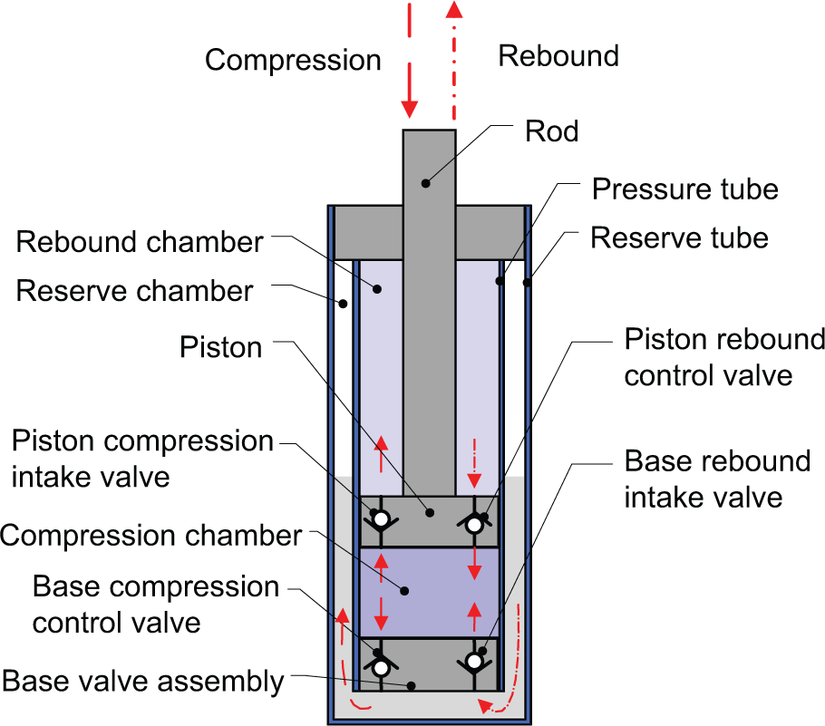
Hydraulic damper working principle.
The action of the piston transfers the liquid surrounding the rod to the reserve chamber. The reserve chamber is partially filled with fluid (oil) and partially filled with gas (nitrogen). The combined volume of the compression and rebound chambers during piston movement changes by an amount equivalent to the inserted, or withdrawn, rod volume. The oil is transferred from the reserve chamber to the compression chamber through the cylinder-end assembly located at the bottom of the compression chamber. Two types of valves, i.e. intake and control valves, are used in a double-tube hydraulic damper to enable liquid flow from the compression to the rebound chamber and from the rebound to the compression chamber.
2.2. Model of a hydraulic damper
The model of a hydraulic damper introduced in this section was derived using the mass flow approach based on the previously presented model. 5 The proposed model formulation facilitates the inclusion of the oil–gas emulsion model necessary for the multi-tube type hydraulic dampers considered in this paper, in which oil surface is exposed to free gas in the reserve chamber. The emulsion model captures the effect of significant changes in oil properties (e.g. bulk module) due to the presence of gas fractions dissolved in the oil. The model assumes constant oil temperature.
The model of a servo-hydraulic test rig is the model developed previously based on a volumetric flow model. 5 This is because servo-hydraulic installations are equipped with accumulators providing separation between gas and liquid volumes using an elastic diaphragm or a floating piston. In turn, oil properties are assumed to be unaffected by the presence of gaseous fraction in the oil and significant changes in the oil bulk module. The model assumes constant oil temperature.
The presented hydraulic damper model has been developed based on the following assumptions: (i) the dependency between density and pressure is nonlinear (oil–gas emulsion); (ii) pressure and density are uniformly distributed in particular chambers; (iii) pressure–flow characteristics of all restrictions are given as monotonic functions; (iv) valves open and close abruptly in a completely symmetrical manner (valve dynamic is not considered); (v) oil temperature is constant; and (vi) the low-amplitude (<10 mm) random excitation is used therefore the stretch effect of the tube due to internal pressure is neglected.
2.2.1 Force equilibrium
The behavior of a hydraulic damper connected with a top-mount can be described by the following equation:
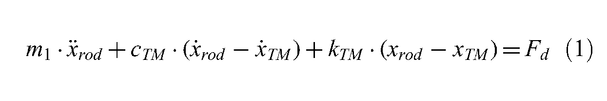
The force Fd generated by a hydraulic damper is obtained by taking the equilibrium of forces acting on the inertial piston-rod assembly into account:9–11
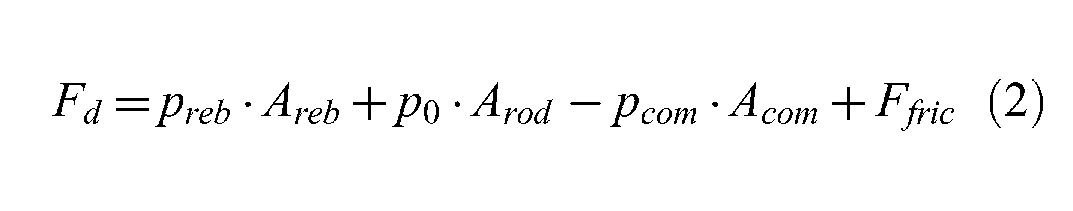
where Arod, Acom, Areb are the areas (m 2 ) of the rod, compression, and rebound side of the piston; pcom, preb are the pressures (Pa) in the compression and rebound chambers; p0 is the atmospheric pressure, p0 = 1 × 10⁵ Pa; and Ffric is the dry friction force between the piston and pressure tube.
The dry friction force Ffric between the piston and pressure tube is modeled as follows:
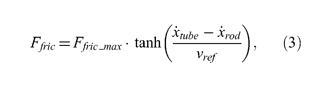
where the friction force Ffric depends on the direction of relative velocity
The proposed friction model uses the hyperbolic tangent function tanh(.), which provides a smooth switching of friction force similar to the measurement data. The maximum friction force Ffric_max is experimentally obtained using a hydraulic damper without valve restrictions for the low reference velocity vref = 0.01 m/s (equation (2))
2.2.2 Model of flow restrictions
Intake and control valves are adjusted to ensure customer specifications regarding the force versus velocity characteristic are met. The flow through a valve system can be modeled either in a (i) first-principle or (ii) data-driven model. This paper takes into account the experimental data-driven model (static pressure-flow curves) which was parametrized for optimization purposes using physical interpretable parameters.
The measured static pressure-flow characteristics of all restrictions are required in the model to capture the relationship between the pressure drop Δp across the considered valve assembly and the volumetric flow rate q through the valve assembly. Czop and Sławik reported the pressure–flow characteristics which were measured on a flow-bench device and used in the model. 5
2.2.3 Damper model
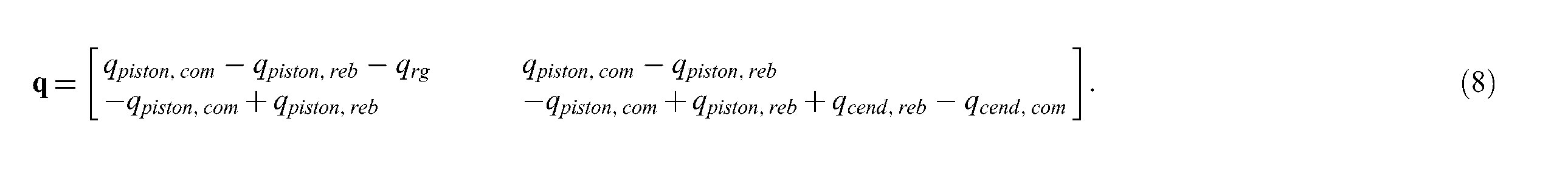
Changes in the oil mass in the compression and rebound chambers are obtained using the following equations:
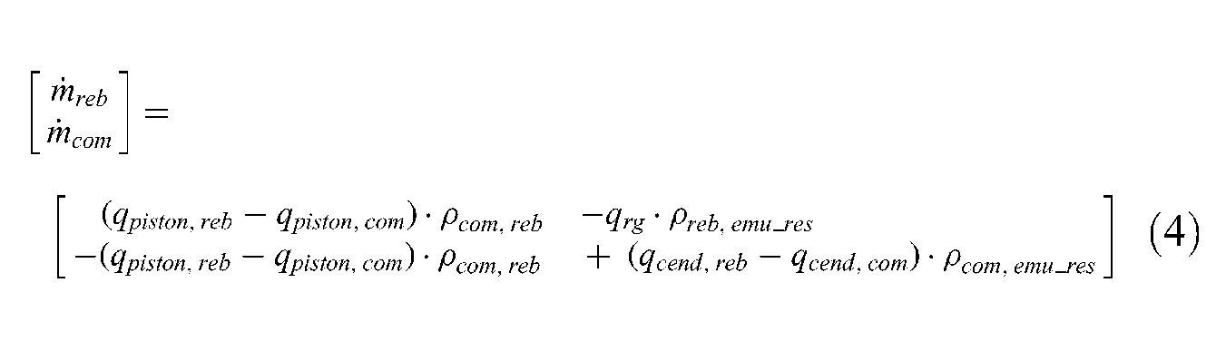
where
Rearranging the mass flow equation and knowing that
the following differential equations are obtained
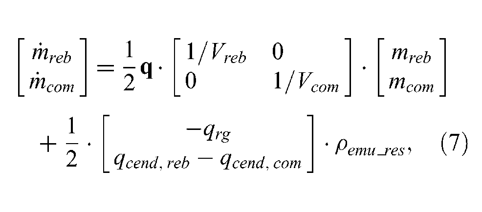
where
The volumes of the Vcom compression and Vreb rebound chambers are obtained with the following algebraic formula:
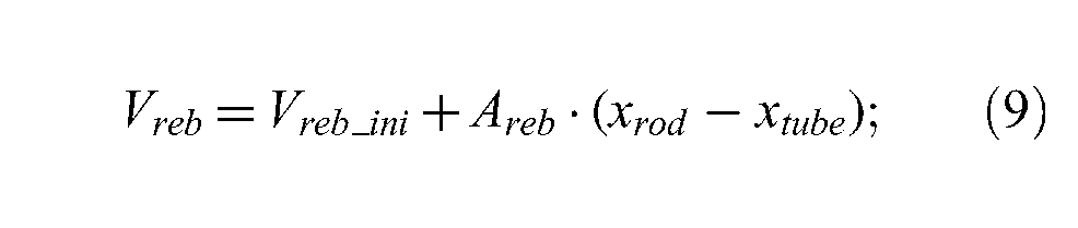
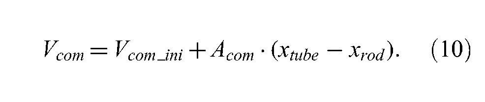
where (xtube–xrod) is the relative movement between the piston-rod assembly and the body of the hydraulic damper, Vreb_ini and Vcom_ini are the rebound and compression chamber volumes at the displacement xtube– xrod = 0. The total oil mass in particular chambers is obtained as follows:
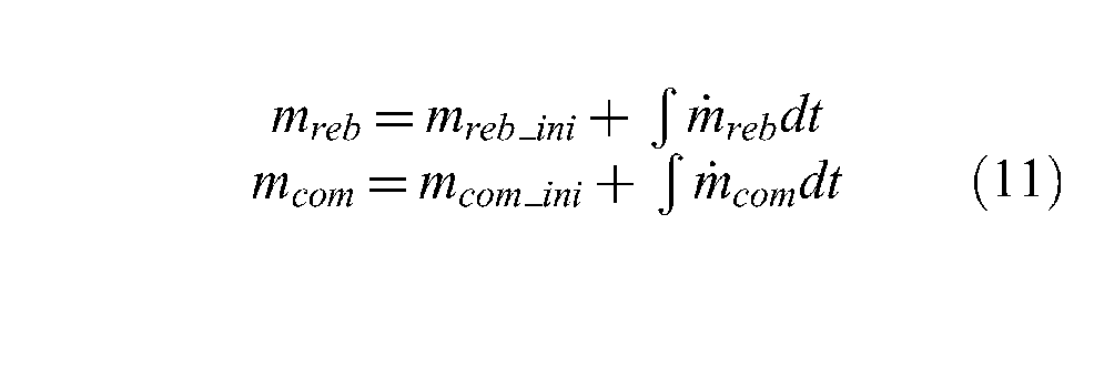
based on the initial oil mass and the mass changes in the rebound and compression chambers. The mass of the oil in the reserve chamber is calculated based on the oil mass balance of the entire hydraulic damper:
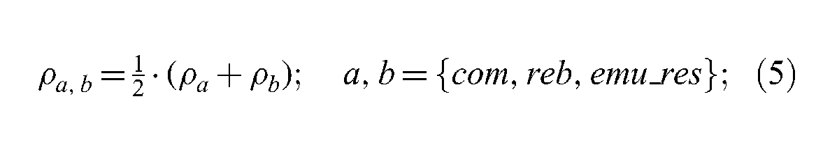
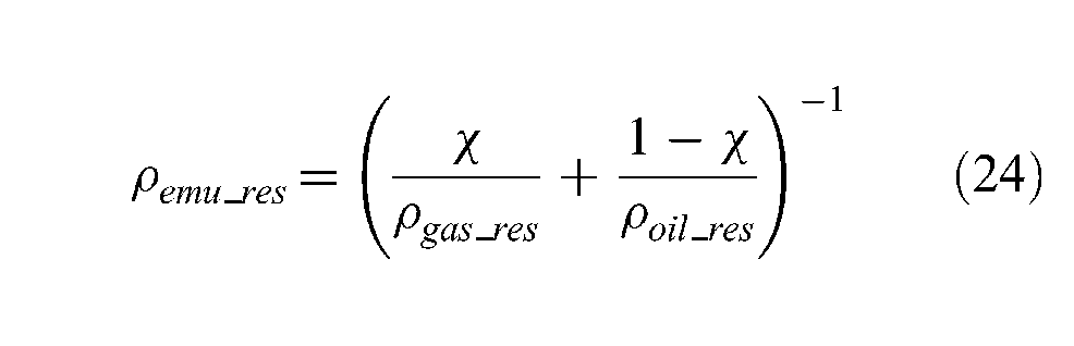
The average density of the oil–gas emulsion in the reserve chamber ρemu_res is a function of the average density of the oil–gas emulsion and gas in the reserve chamber ρres:
The average density ρres can be calculated with the formula

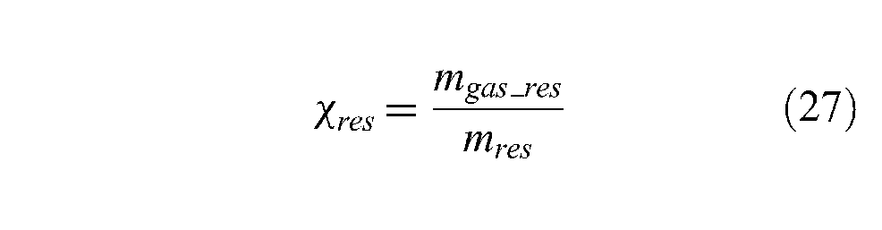
where mgas_res is the mass of free gas in the reserve chamber (kg), memu_res the mass of the oil–gas emulsion in the reserve chamber (kg), memu the mass of the oil–gas emulsion in the whole double-tube damper (kg), mreb the mass of the oil–gas emulsion in the rebound chamber (kg), mcom the mass of the oil–gas emulsion in the compression chamber (kg), and Vres the volume of the reserve chamber (m 3 ).
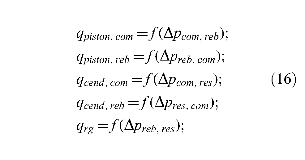
The volumetric flows q through the piston, cylinder-end, and rod guide depend on the pressure drop Δp and are given as static characteristics:
The pressures pcom, preb, and pres can be determined as a function of density
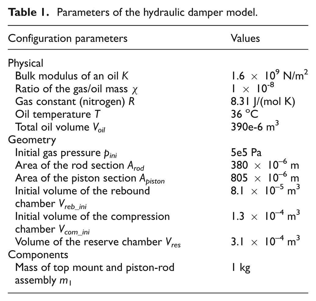
The model parameters are listed in Table 1.
Parameters of the hydraulic damper model.
2.2.4 Two-phase gas–liquid flow model
A liquid that was exposed to a soluble gas (i.e. the liquid had a contact surface with the atmosphere of a gas that can dissolve in it can be in one of three forms: (i) liquid–gas solution, (ii) liquid–gas bubble emulsion or (iii) foam (froth). The physical properties of the liquid–gas solution are not significantly different from the properties of the pure liquid; values of the density and the bulk modulus remain very close to the ones of pure liquid. 13 The liquid–gas solution is, however, prone to bubble formation; when the pressure of the liquid–gas solution decreases, the liquid is no longer capable of retaining all the gas in a dissolved form and so bubbles occur. 13 The presence of gas modifies the density and bulk module of the oil and causes a delay in the build-up of damping force and the hysteresis loop in the force–velocity response. In the case of the oil and gas-bubble emulsions, it is assumed that the volume of gas bubbles is significantly smaller than the volume of the liquid. On the other hand, the foam (froth) is the state of the gas–liquid mixture in which the volume of the bubbles of gas is larger than the volume of the liquid.
Dixon provides a theoretical overview of the emulsification and de-emulsification processes. 12 The homogeneous emulsion model assumes that the particles of gas and the liquid have the same velocity and are in the same thermal equilibrium. Additionally, the solubility of gas in liquid is constant and equal in all chambers. The density ρ of the oil–gas emulsion forming in a hydraulic damper is obtained with use of the following formulas: 12
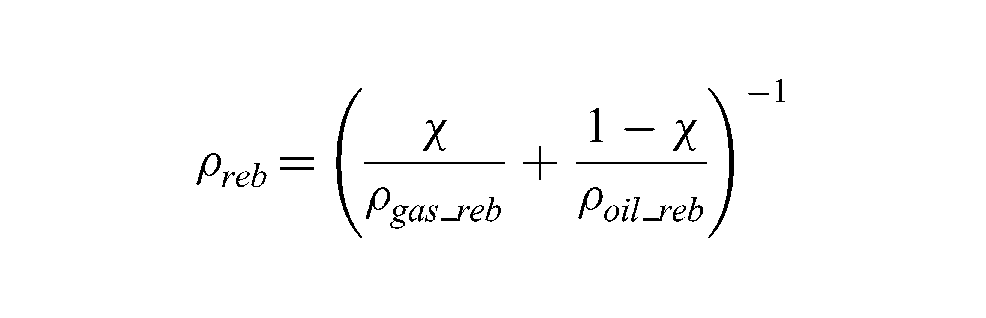
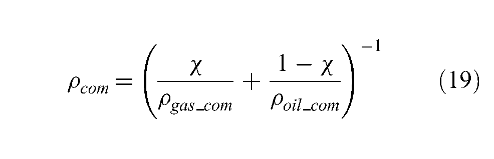
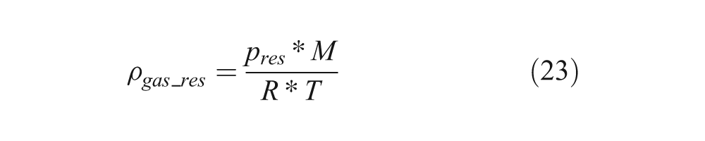
where the χ value is a ratio of the mass of gas to the total mass of oil and gas present in an emulsion. The initial guess of the χ value was evaluated with Henry’s law, 12 then refined using the measured force–displacement curves. The density of gaseous fraction of the oil–gas emulsion is obtained using an ideal gas equation:

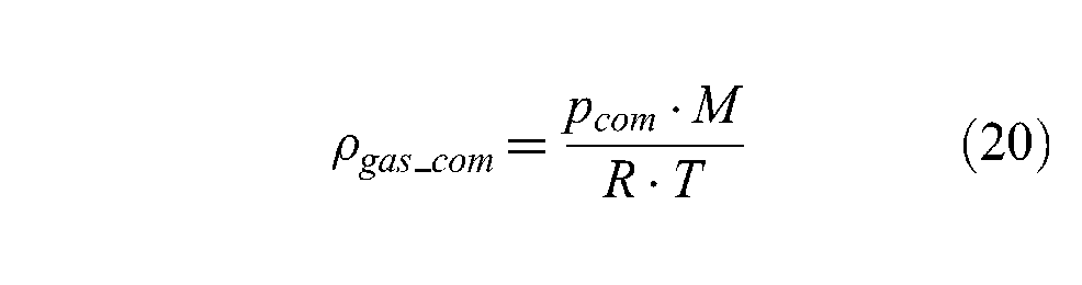
where M, R, and T are the gas constant, the molar mass of gas, and the temperature, respectively. The pressure in the compression and rebound chambers is determined as follows:
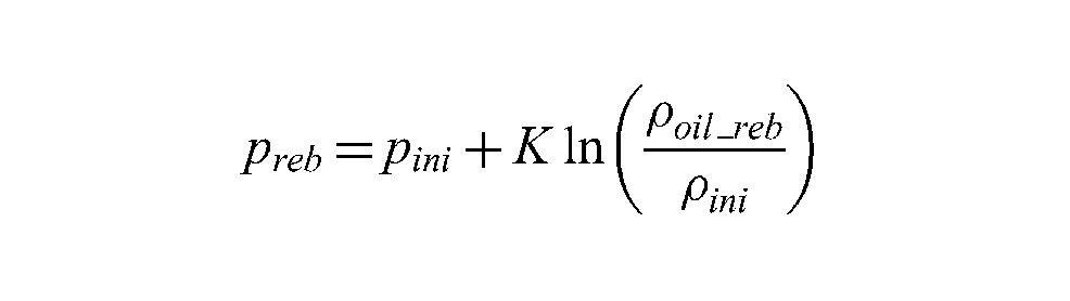
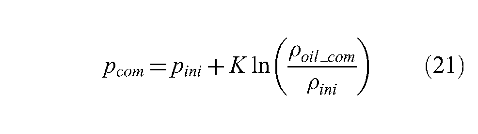
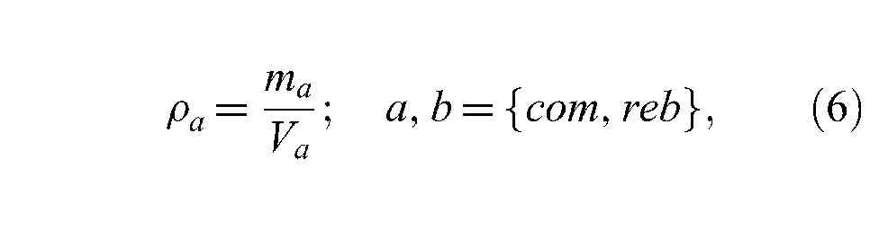
The density of the emulsion is then calculated as a ratio of the oil mass in the chamber and the volume of the chamber. The resultant pressure–density relation of the oil–gas emulsion is presented in Figure 2.
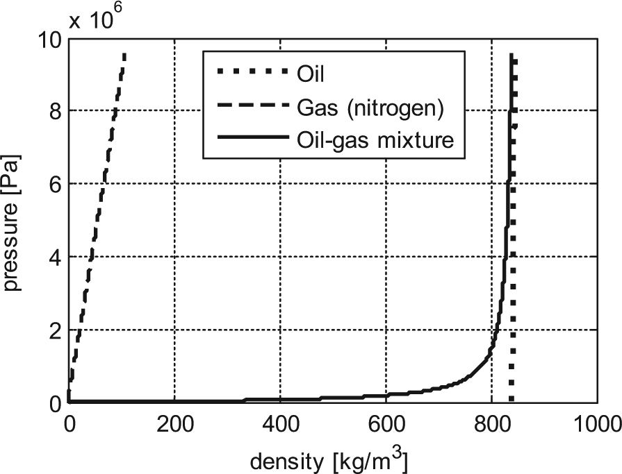
Density–pressure relation for gas (isothermal), oil, and oil–gas emulsion.
The reserve chamber contains a free gas and the oil-gas emulsion, therefore more extended calculations are required (Figure 3).
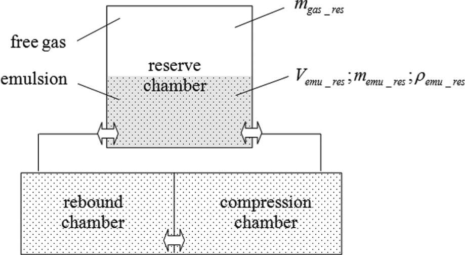
Schematic presentation of the content of hydraulic damper chambers.
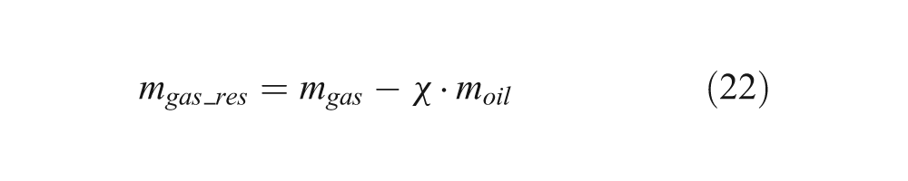
The mass of free gas in the reserve chamber is calculated using the assumption that the χ value is equal in all chambers:
The density of free gas and gas dissolved in the emulsion occupying the reserve chamber is determined as:
The average density of the oil–gas emulsion in the reserve chamber is calculated based on the obtained densities, as follows:
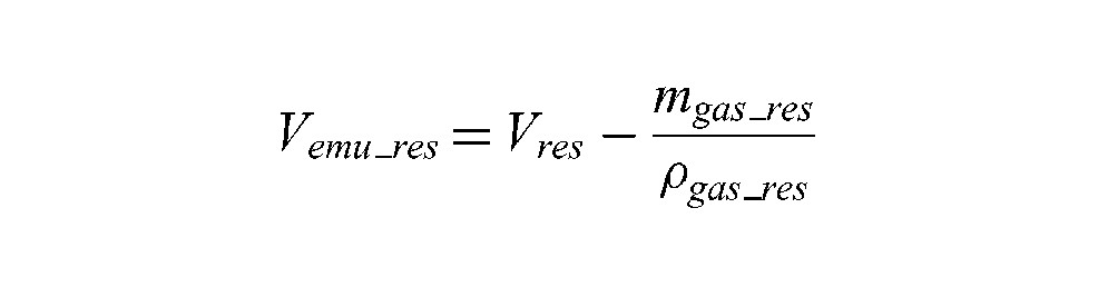
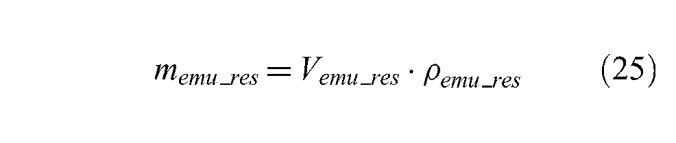
Using the calculated values, the volume Vemu_res and the mass memu_res of the oil–gas emulsion in the reserve chamber are:
Finally, the average density of the oil–gas emulsion and gas in the reserve chamber is calculated using the following formula:
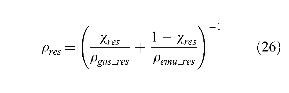
where
2.3. Combined model
The hydraulic damper and the servo-hydraulic tester models were coupled and tuned. A hydraulic damper is rigidly attached to the main frame of the servo-hydraulic tester through a top fixation (the load cell) and a top mount (Figure 4). The bottom end of the hydraulic damper is rigidly connected to the rod of the hydraulic actuator. The equivalent system of the servo-hydraulic tester is formulated as a serial connection of mass, damping, and stiffness equivalent elements. In this model, the coefficients representing the damping and stiffness of a hydraulic damper and a hydraulic actuator are nonlinear, and their values result from the nonlinear hydraulic flow equations presented in the previous sections.
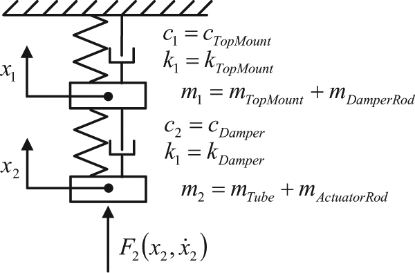
Equivalent stiffness–damping representations of the combined system of a hydraulic damper and a test-rig.
The fundamental modes of the complete system (hydraulic damper + tester) are covered by the proposed model. The complete force balance is given by the following differential equations:
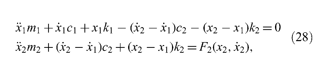
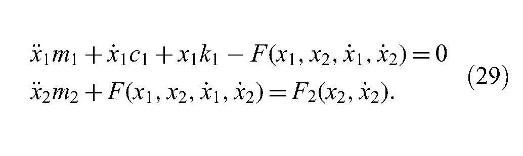
Taking into account the nonlinear term of damper force F, which depends on the relative displacement (x2−x1) and its velocity, equation (28) can be written in the following form:
The mass distribution results from the spatial discretization of the construction, i.e. the actuator rod, the hydraulic damper tube, and the rod attached to the traveling part of the top mount.
3. Key parameters of a pressure–flow characteristic to be optimized
A double-tube damper consists of four valve systems which mutually interact contributing to the total damping force of a hydraulic damper. The damper is equipped with two intake and two control valves (Figure 1). The control valves determine the damping force characteristic of a damper, while the intake valves should ideally not generate any damping force, allowing the flow in one direction and stopping in the reverse direction. Nevertheless, the base intake has fewer possibilities for optimization since it is a coil–spring valve whose tunability is limited to the opening stiffness and spring preload. Therefore, the piston intake valve was chosen to be optimized to reduce the vibrations of a hydraulic damper. The goal of optimization is to obtain a pressure–flow characteristic of a valve system which minimizes the vibration level produced by a hydraulic damper while maintaining the same damping force.
A typical piston intake valve is characterized by the pressure–flow characteristics, as presented in Figure 5. The controller regulates the flow through the valve allowing the pressure-flow characteristic of a valve to be captured. The pressure is a differential pressure measured before and after the flow tool evaluating the pressure drop across the valve assembly for a given flow rate. The pressure–flow characteristic and its model are both shown in Figure 5.
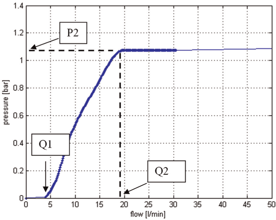
Parametrization of the valve pressure–flow characteristic.
The model of the pressure–flow characteristic is formulated based on the three key design parameters indicated in Figure 5. These parameters were formulated based on the engineering experience that they can be easily translated into the valve design properties.
The beginning part of the characteristic, up to 17 l/min, is the bleed region when the valve disc is closed and oil flows through the initial orifices (bleed discs) or notches in the valve seat. The first design parameter Q1 defines the valve flow when the intake valve is still closed. The second design parameter Q2 defines the valve blow-off threshold when the built pressure is enough to separate the disc from the valve seat. In this point pressure P2 acting on the valve is in equilibrium with the disc spring preload initially applied to this valve. The design parameter Q2 is defined by the area of the bleeds given in squared millimeters. The flow is proportional to the area. It is assumed that the range for this parameter is from 0.1 to 9.5 l/min. When the valve opens, stiffness of the valve spring controls the height of the opening, balancing the pressure. In this region pressure increases slowly while flow rate increases significantly until the moment when the valve is fully opened (outside the range of measurements).
The optimization goal is to find a trade-off among those three parameters. Two alternative methods were proposed in order to find the optimal parameter values, namely the quick-and-dirty model surface response and nonlinear programming method.
4. Optimization with the use of design of experiment plan
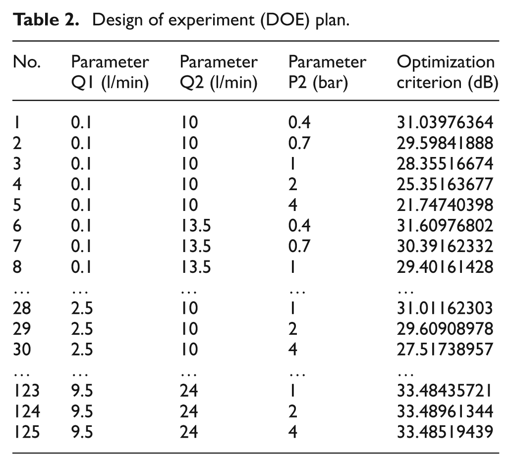
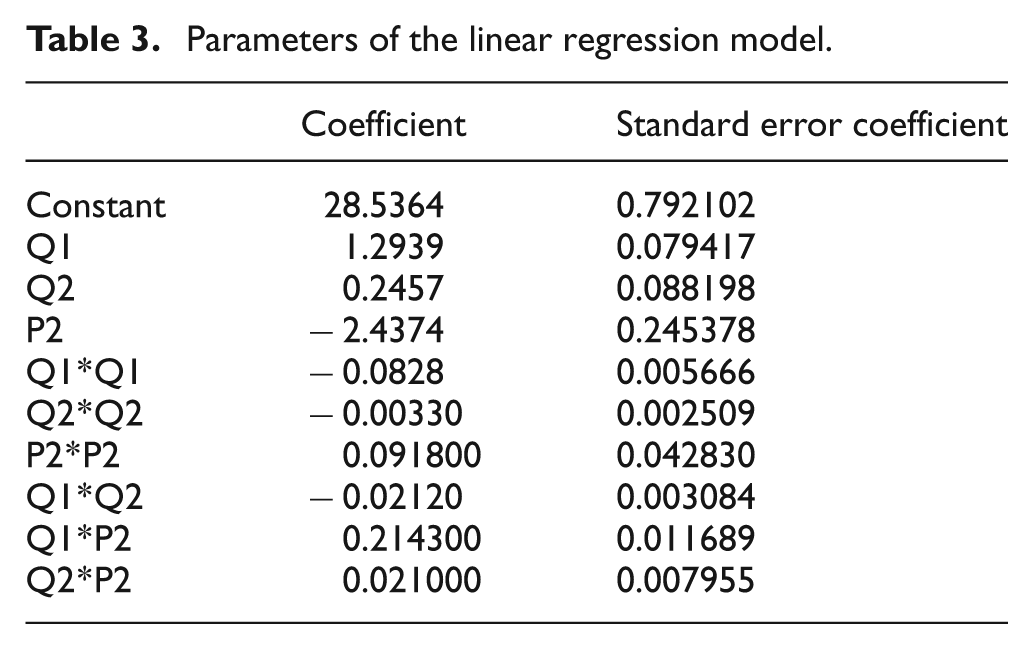
Design of experiment (DOE) is a quick-and-dirty method for simultaneously investigating the effects of multiple variables on an output variable (response). The experiments consist of a series of simulation runs (Table 2), in which input variables are modified according to the experiment scenario. DOE was prepared using MiniTab statistical software. 8 The ‘response surface design experiments’ option available in MiniTab was chosen to model the influence of parameters of the pressure-flow characteristic on the maximum vibration level (peak value) in the power spectrum obtained using a piston-rod acceleration signal. The DOE plan includes three independent parameters Q1 (l/min), Q2 (l/min), and P2 (bar). The vibration level is expressed in the dB scale. An optimization model was developed using MiniTab statistical software using linear regression. 8 The coefficients of the model are reported in Table 2. The model fit to simulation data achieved a high value of 94.29%.
Design of experiment (DOE) plan.
The optimization process was validated regarding its correctness based on the following diagnostic measures and characteristics (Figure 6):
normal probability plot to detect abnormality;
histogram of the residuals to detect multiple peaks, outliers, and abnormality;
residuals versus the fitted values to detect non-constant variance, missing higher-order terms, and outliers,
residuals versus order to detect the time-dependence of residuals. The measures indicate normal distribution of residuals without any outliers or other abnormalities and confirm good model fit to the data.
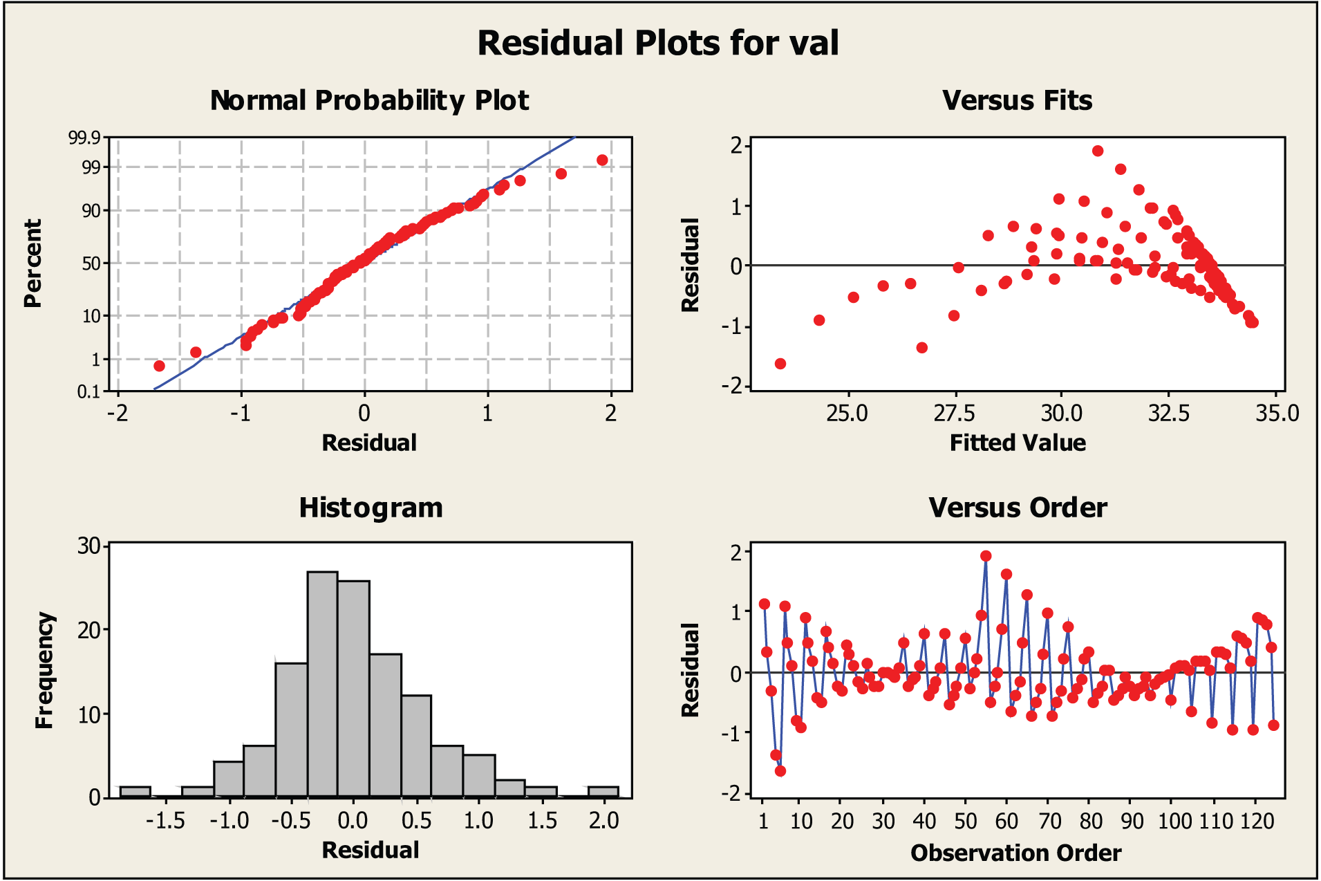
Diagnostic check of the optimization model based on the model residuals.
The selection process of optimal design parameters is performed visually based on the contour plots of the best-fit surface, the so-called response surface, created separately for each set of DOE measurements. The response surface, drafted on the basis of the linear regression model equations, indicates the direction in which the values of design parameters should be changed to minimize the vibration level. The surface has four dimensions; therefore it was decomposed into three two-dimensional sub-surfaces (Figure 7). The top-left sub-surface recommends minimizing Q1 and Q2 to lower the vibration level. The top-right sub-surface recommends maximizing P2 and minimizing Q1 to lower the vibration level, while the bottom-left sub-surface recommends maximizing P2 and minimizing Q2 to lower the vibration level, however, the contribution of the P2*Q2 interaction is less significant compared to the previous ones.
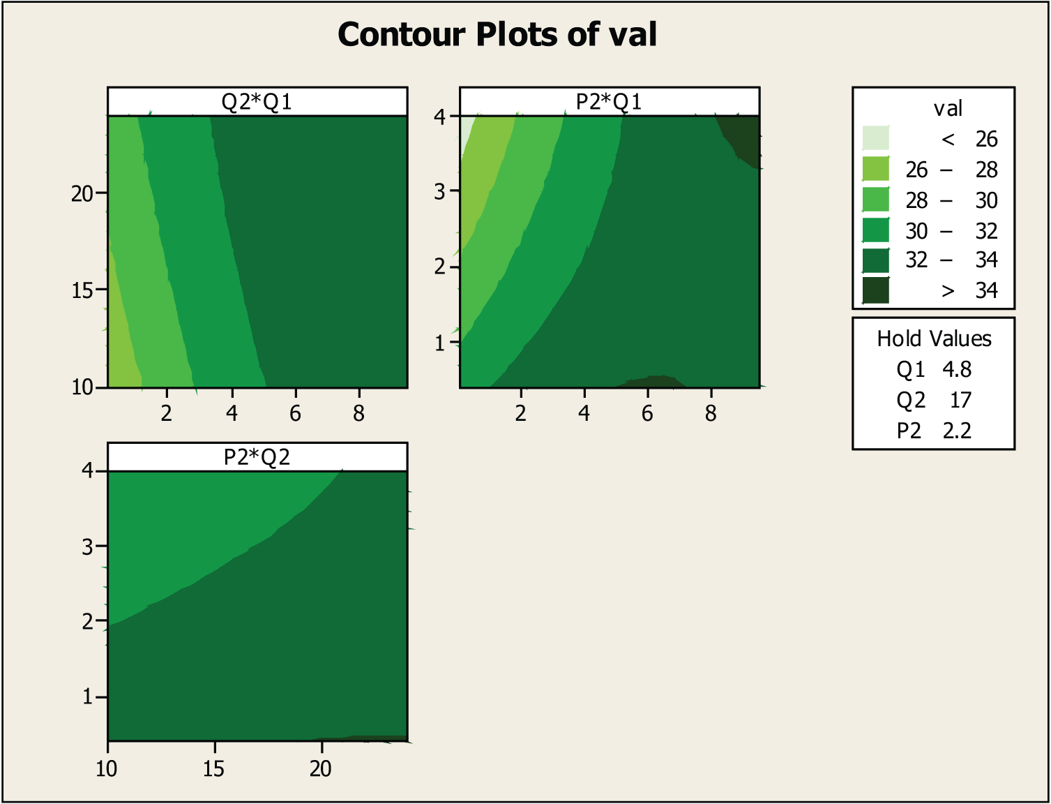
Results of application of the response surface method presented with the use of 2D sub-surfaces.
In the case of higher-dimensional parameter spaces, other visualization techniques are used,9,14 as presented in Figure 8.
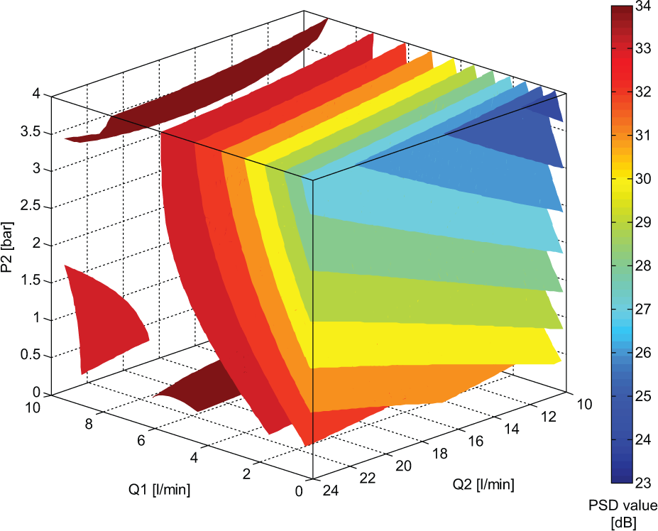
Results of application of the response surface method presented with the use of 4D surface.
The optimal solution is achievable for Q1 = 0.1 l/min, Q2 = 10 l/min, and P2 = 4 bar. The parameter values achieved the boundary limits indicating an improvement direction. Nevertheless, in typical applications, vibrations are minimized to maintain a trade-off among acceleration level, required ride comfort, and valve durability. In turn, the optimal solution has to be adapted to many constraints resulting from available standardized manufacturing components and customer preferences.
The Pareto graph in Figure 9 provides a ranking of model variables and their interactions plotted on the basis of the standardized model error reported in Table 3.
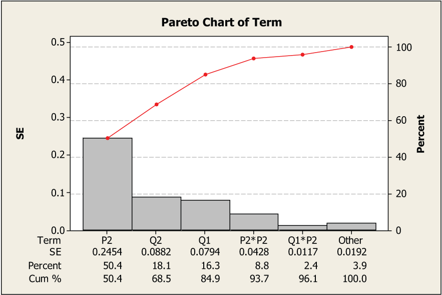
Ranking of model variables and their interactions.
Parameters of the linear regression model.
The graph indicates which variables are the most sensitive in terms of achieving improvements in reduction of the vibrations.
5. Optimization with the use of nonlinear programming method
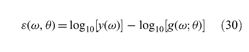
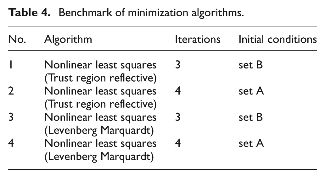
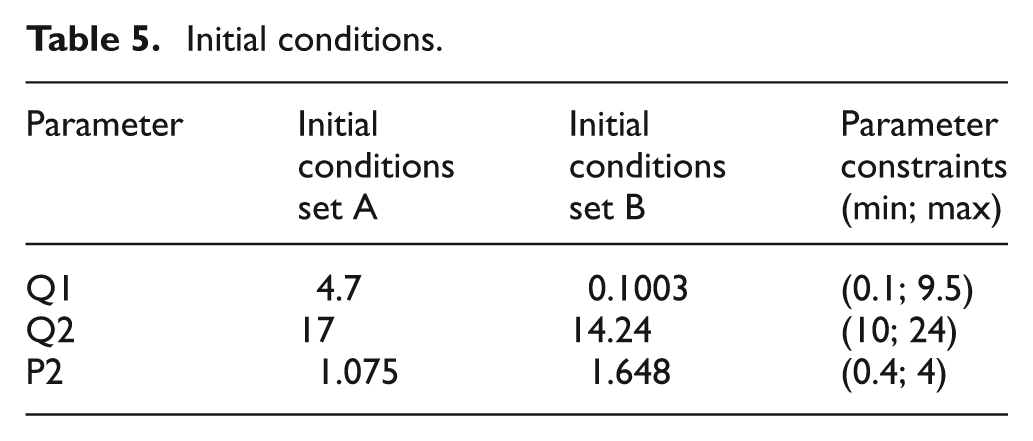
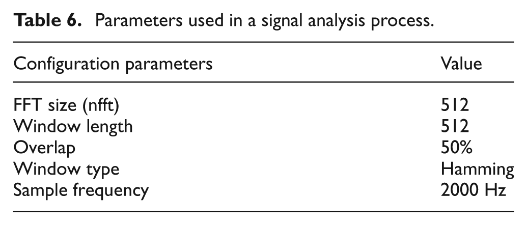
Nonlinear programming was used in order to minimize the error function between the hydraulic damper model prediction and its measured response. The optimization was conducted using combinations of second-order methods (Table 4)15–17 and two sets of initial conditions (Table 5). The sum of squared errors was used as the error criterion to evaluate the fit of the model to operational data in the frequency domain based on the piston-rod damper acceleration. 5 The acceleration power spectrum was obtained using a signal analysis process, as shown in Table 6. The objective function is defined as follows:
Benchmark of minimization algorithms.
Initial conditions.
Parameters used in a signal analysis process.
The optimization process was validated regarding its correctness based on the following diagnostic measures and characteristics:
The model parameter trends visualized in the function of iterations required to achieve the optimization algorithm-stop conditions are the so-called convergence trajectory plots (Figure 10). They are used to evaluate the robustness of the algorithm based on the smoothness in approaching the algorithm stop-criterion (Table 4).
Repeatability tests when the initial guess values of the model parameters are changed to examine the robustness of the convergence algorithm regarding the repeatability of the estimated parameter values. This test quantifies resistance of the algorithm to local minima (Table 5).
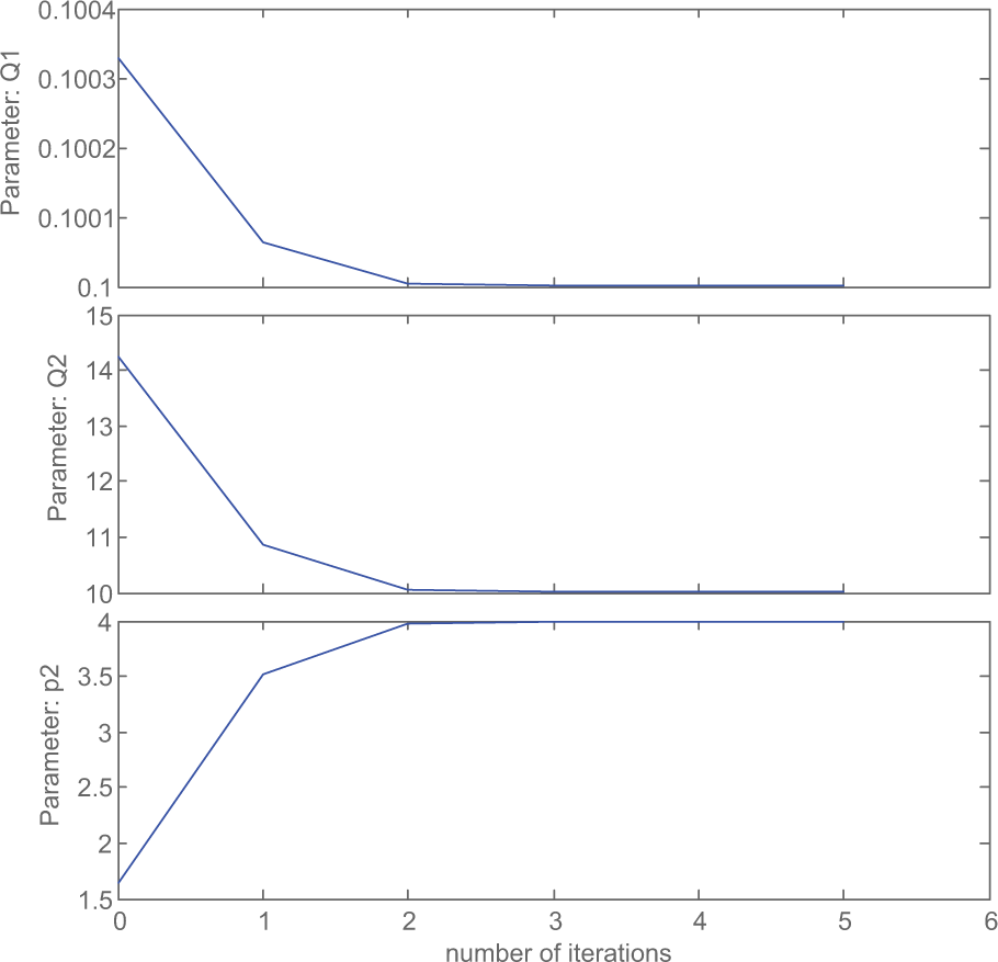
Convergence trajectory plots (set A, Table 4).
The convergence trajectory plots show trends towards constant values of the parameters, which correspond to convergence towards the minimum of the criterion function, within a few iterations (Figure 10). The same optimal solution as in Section 4 was found, i.e. Q1 = 0.1 l/min, Q2 = 10 l/min, and P2 = 4 bar. The optimization was repeated with other sets of initial values and achieved the same solution (Tables 4 and 5). Both nonlinear programming algorithms have proved resistant to the initial conditions (Table 4). The convergence process was longer by one iteration using Set A of initial conditions (Table 5).
6. Validation of the optimized valve design
The simulation model used to find optimal pressure–flow characteristics has to be accurate enough and therefore requires operational validation. Validation was performed on a Hydropuls® MSP25 servo-hydraulic test-rig, equipped with an IST8000 electronic controller (Figure 11). The test rig was used to load a hydraulic damper and capture its dynamic characteristics, i.e. displacement vs. force. Data acquisition was performed with an 8-channel ICP amplifier manufactured by LMS. The test rig is equipped with an oil supply system (the so-called servo-pack) that provides a pressure of 28 MPa at a flow-rate of 90 l/min. The actuator provides a 25 kN force at the rod, while the maximum stroke is 250 mm at the maximum achievable velocity of 3 m/s. The actuator rod is coupled to the adapter, which transfers the force to a hydraulic damper mounted on a test rig.
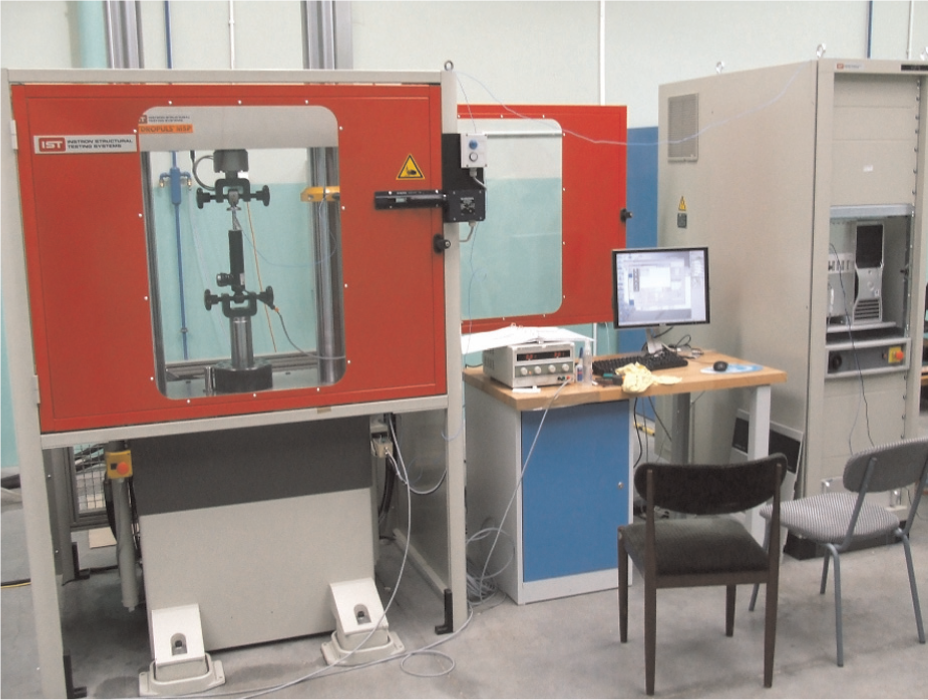
A servo-hydraulic test-rig used in experimental investigations.
The main components of the servo-hydraulic system are the hydraulic actuator with an integrated displacement transducer in a piston-rod assembly (IST-Schenk) and the three-stage servo-valve system. The test rig is equipped with a PID-FF controller. The feed-forward (FF) section in this controller passes a proportion of the command signal to the controller output through a high-pass filter to block the command mean level. Different control settings are used depending on the type of excitation signal. The excitation signal is converted into a voltage applied to the servo-valve, which controls the amount of oil supplied to the chambers of the actuator.
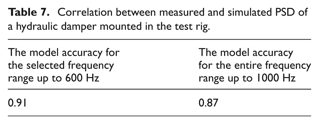
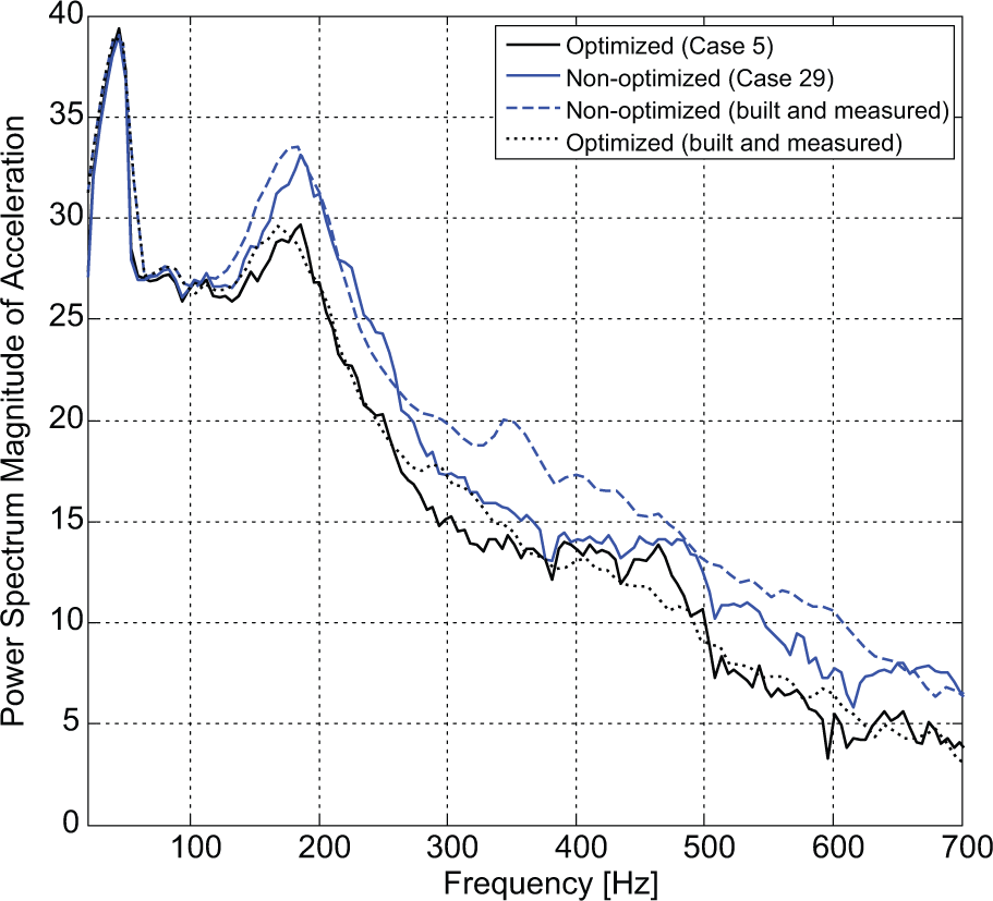
The validation of the combined model of the hydraulic damper and the servo-hydraulic tester was performed with the use of a pink noise signal of the maximum peak-to-peak amplitude of 10mm and frequency band 0–50 Hz was used to excite wide-band vibrations of a hydraulic damper similar to those in road conditions. The high-frequency results obtained from measurements and simulations were compared in the frequency domain and are evaluated in Table 7. The results are shown graphically in Figure 12.
Correlation between measured and simulated PSD of a hydraulic damper mounted in the test rig.
The results of simulation experiments were used as guidelines to build the experimental pressure–flow valve characteristics to meet the recommended changes in parameters. Two approximated valve settings were built and measured, namely (i) reference not-optimized (close to the Case 29 from Table 2) and (ii) optimized setting (close to the Case 5 from Table 2). The non-optimized and optimized pressure–flow characteristics are presented in Figure 13.
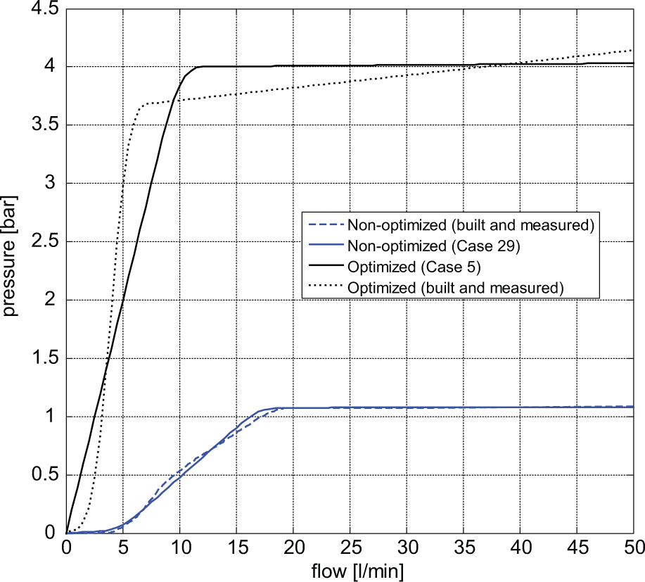
The hydraulic damper was equipped with a modified (optimized) valve to quantify the operational improvements in reducing the vibration level. The comparison is shown in Figure 13.
The hydraulic damper equipped with the optimized piston intake valve produced lower vibration compared to the reference, not optimized, valve. The difference of 4 dB is significant since it is measured within an uncertainty tolerance of measurements of 1.5 dB in the frequency range of interest between 100 and 250 Hz.
7. Summary
The paper describes a method towards reduction of vibrations produced by hydraulic dampers without affecting the damping force characteristics. The paper applies the model-based approach to obtain the optimal pressure-flow characteristics by simulations conducted with the use of coupled models including the damper and servo-hydraulic tester model. The presence of the tester model is required due to high non-linear coupling of the tested object (damper) and the tester itself to be used for noise evaluation. The models replicate, by means of simulation, the process of vibration evaluation used in the automotive industry as an alternative to vehicle-level tests. 5
This paper proposes two alternative optimization methods, namely a quick-and-dirty method based on a design of experiment (DOE) plan and a nonlinear programming method based on the minimization of criterion function. In both cases, the trends in design parameters are obtained to provide an input to a designer and test engineer to prepare the best valve design and make the choice of the optimal valve design. The proposed optimization methods are based on the model which should include relevant physical phenomena in order to trend valve design physical properties. This aspect is discussed in detail by Czop and Sławik. 5 The physical phenomena not included in the simulation model cannot be taken into account in the valve process optimization. This states the major limitation of the method.
The optimization process was defined through five objectives which were addressed in the paper. The first objective was to develop a double-tube damper model. The model was adapted and customized for a double-tube hydraulic damper based on earlier work, 5 tuned and validated using available measurement data. The second objective of this work, namely define key parameters of the pressure–flow characteristic was fulfilled by determining three parameters, Q1, Q2, and P2. The interpretation of these parameters is given in Section 3. The third objective was to apply two optimization methods to lower vibrations of a hydraulic damper. Two methods were used and discussed in the fourth and fifth sections. The optimal tuning parameters minimizing damper vibration level were obtained based on the response surface plots and using the nonlinear least squares minimization algorithm completing the fourth objective. The fifth objective was to perform an experimental case study to show if the proposed optimized pressure-flow characteristic decreases the vibration level. The hydraulic damper equipped with the optimized piston intake valve produced lower vibration compared to the original, not optimized, valve. The difference of 4 dB is significant since it is measured within an uncertainty tolerance of measurements of 1.5 dB in the frequency range of interest between 100 and 250 Hz.
The final solution is not only a mathematically obtained optimum, but most importantly, it addresses customer preferences and manufacturing constraints, i.e. valve parameters have standardized discrete values, such as disc diameters. Nevertheless, the availability of the optimum function is a great advantage in a valve design process since the choice of a new valve configuration can be immediately recalculated providing a starting point in further optimization or supporting the sensitivity analysis process.
Future investigations are planned to focus on deployment of a new analytical tool in the engineering development process which allows automatic performance of the optimization process.
Footnotes
Funding
The authors gratefully acknowledge the financial support of the research project: N N502 087838 funded by the Polish Ministry of Science (MNiI) and RGH-9/RMT0/2012 founded by the Rector of Silesian Technical University.