
Abstract
The amount of food transported long distances in reefer containers is constantly increasing and so is the cost per mile because of rising fuel prices. One way to reduce the cost is to minimize the energy consumed by reefer containers through a better controller but in order to achieve this a fast and flexible simulation model is needed for controller development. The simulation model may also be used for developing fault diagnosis methods for the reefer container and thereby further lowering costs by reducing the amount of functioning spare parts that is replaced and by providing early warning for faults enabling preventive maintenance. In this paper the feasibility of using different simulation methods is assessed with the goal of identifying a fast but accurate method that works well in a multi-rate environment. A modular multi-rate simulation environment for a dynamical system consisting of components with different dynamical speeds is presented with an improvement of previous results. The simulation speed is improved by 350% with no reduction in the accuracy of the solution, by substituting the M
1. Introduction
Reefer containers are used extensively to transport food all over the world and by mid-2008 there was a worldwide fleet of 11.4 million twenty foot equivalent (TEU) predicted to grow by 69% to 19.3 million TEU by 2013, according to the Reefer Shipping Market Annual Report. 1 The container cargo market is highly competitive and therefore it is interesting to examine any possible means of lowering the total cost of ownership (TCO), which covers the cost of initial procurement and operation during its lifetime, of a reefer container. The average lifetime expectancy for a reefer is 12 years and the cost of procurement is small compared to the cost of inspection, repairs and energy over the lifetime of the container. This of course means that there is a potential for lowering the TCO through a reduction of these three factors; that will be clarified in the following. Before every trip a reefer must complete a pre-trip inspection (PTI) test which is a self test where the container tests that its cooling capacity is as specified and that there are no other obvious problems. This requires that the container is taken to a special PTI area on the harbor where it is plugged in and the PTI test is started by an operator, for a fee that covers handling and power. The PTI test is executed in this way because it is a programmed sequence that requires the container to be empty so that it may change the temperature set point and cooling capacity without risk of damaging the cargo. But if this self check could be done by examining the relationship between control signals and sensor inputs without changing set point or cooling capacity it would be possible to avoid the PTI test because the container controller would be aware of the capabilities of the container at all times. This self check may be extended further from covering just the available cooling capacity and elementary faults to accurate detection and identification of the majority of likely failures on the container, thereby lowering the time and effort needed to carry out maintenance during the trip. It can also enable early warning on errors that increase over time, which opens up the possibility to carry out preventive maintenance between trips where parts that are close to failing can be replaced, and that is always preferable over repairs that have to be carried out at sea while the container is in use. These measures would increase reliability due to better and in-time maintenance of the container and thereby also decrease the chance of losing cargo due to system failure. But in order to accurately identify faults it is necessary to use model- or observer-based fault detection and isolation (FDI) techniques and for that an accurate model that can be embedded in the container controller is needed. In general, a fairly high-fidelity model can be required in order to detect certain types of fault. Some faults might require a good static model fit, whereas other faults might require the model to fit well dynamically. 2 In this paper, we will mainly focus on the latter class of faults.
The average power consumption of a reefer is 3.6 kW per TEU 3 and assuming an idle time of 50% the total power consumption of the world’s reefer container fleet is above 20 GW. In recent years the shipping business has been looking into ways to cut costs, and the energy consumed by reefers, that earlier was deemed insignificant compared to the main engine energy consumption, has now come into focus. There are two ways to lower energy consumption: by changing the mechanical design of the reefer and the cooling system or by optimizing the way it is controlled. This paper uses the Star Cool container 4 as an example but the mechanical design of this reefer is already nearly optimal, leaving control optimization as the best option for efficiency improvements. The refrigeration unit is controlled by a microprocessor with a control algorithm already optimized for energy efficiency, on the short term. On the long term, however, the potential for energy savings is large if daily variations in ambient temperature are exploited by cooling more when the ambient temperature is low and less when it is high.5,6 This method ‘stores’ some cooling in the cargo during low ambient temperature periods when refrigeration system efficiency is higher and takes it back when the ambient temperature is high and refrigeration system efficiency is lower. The cargo in a reefer container is the single largest thermal capacitance of the system with a time constant that is several orders of magnitude higher than the smallest time constant of the refrigeration system dynamics, which yields a very stiff system. Controller development is an iterative process where a design is tested, evaluated, modified and tested over again and again until a satisfactory result is achieved. On a system like this the time taken can be very long because a test must last several days, due to daily temperature variations and since the system in general has large time constants. If many iterations are needed the time required will be too much and too expensive. Therefore a simulation model is needed to speed up the iterative cycle, and in order to optimize the controller with respect to energy consumption the model must capture both the dynamics of the cargo and the refrigeration plant. The control optimization problem for the reefer container is to keep the cargo within certain temperature limits while using as little energy as possible. Because the efficiency of the refrigeration system is inversely proportional to the ambient temperature and the ambient temperature cycles during a day it is beneficial to apply the cooling when the ambient temperature is at its lowest and use the cargo mass as a ‘storage’ for cooling. This will however require that the simulator and the model are stable, fast, have adequate accuracy and are computationally light-weight enough to run on an embedded system.
There exist many different modeling and simulation tools where models composed of different components may be simulated numerically and in the following a few general-purpose simulators and energy system simulators are described.
Within the field of energy system simulation the modular approach is well known and has been used in for example the simulation environment TRNSYS 7 for more than 35 years to simulate the behavior of a composition of system components over time, using a numerical solver. TRNSYS provides a library of common energy system components that may be combined using a custom system description language.
Another approach is used by
Fault detection and estimation has been shown to work well for refrigeration systems and in Yang et al. 12 a complete FDI approach consisting of an extended Kalman filter and a bank of unknown input observers are described. The combination is shown to have detection and identification capability for sensor and parametric faults on a refrigeration system but it depends on an accurate model for design of the extended Kalman filter and the unknown input observers.
In Kübler and Schiehlen 13 is a modular multi-rate approach where the components may be simulated by different solvers. The component interconnections are managed by a time-discrete linker and scheduler that connects the inputs and outputs of the components and exchanges data at discrete time instants. The advantage of this approach is that it is possible to combine simulators from multiple domains in science and engineering that were not originally designed to work together. Coupling systems with different dynamical behavior with discrete-time linker algebraic loops may cause instability and in Kübler and Schiehlen 13 this problem is described and a method that guarantees stability when algebraic loops are present is proposed. The modular approach has several advantages: it is faster to build a new simulation model from a library of components than starting from scratch and it is also easier to maintain because the code is naturally divided and therefore less likely to be entangled across component models. Simulating a stiff system as a monolithic block has some drawbacks especially under changing conditions on the fast states, 14 because the stiff solver must evaluate the entire system in steps small enough to achieve satisfactory accuracy on the fast states. This is however more than adequate for the slow states and therefore many of the calculations done on them is essentially a waste of computer power. A way to lessen this problem is to convert the ODEs of the fastest states into algebraic equations,14,15 but this can not be used on all states in the current application because too much precision is lost. Another way of reducing the computational load is by using a multi-rate simulator that divides the model into components by their dynamical speeds and thereby yields a significant increase in speed, as shown by Howe 16 and Pearce et al., 17 because slow components are no longer simulated at an unnecessary small step size. In Sørensen and Stoustrup 18 a modular multi-rate simulation environment for simulations of a refrigeration container was described and the theoretical increase in speed was calculated.
For the reefer container application there is a need to simulate the model in small single steps in order to incorporate an external controller, and this is possible with the modular multi-rate approach. An attempt is made to quantify the impact of the multi-rate method on speed and accuracy through multiple simulation experiments on the refrigeration system using different simulator configurations on the refrigeration container model and comparing the results. Furthermore, an attempt is made to increase the simulation speed by using a simple solver tailored for the problem at hand instead of
This paper presents a simulation environment for
2. Methods
This section investigates the benefits and disadvantages of multi-rate and monolithic simulation methods applied to a modular model of the Star Cool refrigeration container, with special emphasis on finding a simple solver that is suitable for implementation on an embedded platform. The simple solver should be able to simulate the model with a precision that is adequate for FDI and for the model to be used as an observer for a model-based controller. Furthermore it must be able to simulate the model in short steps such that it can produce an output at regular intervals that may be used by the FDI and control algorithms on the container controller.
2.1. Refrigeration system model
The model of the Star Cool refrigeration container is used for development, testing and validation of control and fault detection algorithms and therefore the model reflects the system properties that are important for these tasks. The salient properties are the dynamics of the refrigeration system used for control of the evaporator and the dynamics of the container walls and cargo that are relevant for control of the compressor speed. The equations are based on first principles where infinitesimal terms that have little impact on the accuracy or stability of the solution have been removed. This results in a set of mainly first-order equations that due to the highly nonlinear relationship between evaporation temperature and pressure of the refrigerant have varying time constants. One good thing about a refrigeration system is that while operating within the normal limits for the system it settles at a steady state when the control inputs and ambient conditions are steady. Therefore the accuracy of the model is adequate if the equations can capture the varying rates of exponential decay towards an input-dependent steady state. The system has the property that the slow states are isolated in the component that models the container walls and the cargo, and the fast states are present in five different refrigeration system component models. The refrigeration system is divided in components because it is easier to maintain code that is divided in modules with clean interfaces but it also gives the advantage that each component model can easily be substituted by another component if needed. This division also enables the use of custom solvers for each component, depending on what is better suited to the component. A schematic of the refrigeration system is shown in Figure 1 and the details of the system model have been described in Sørensen and Stoustrup. 18
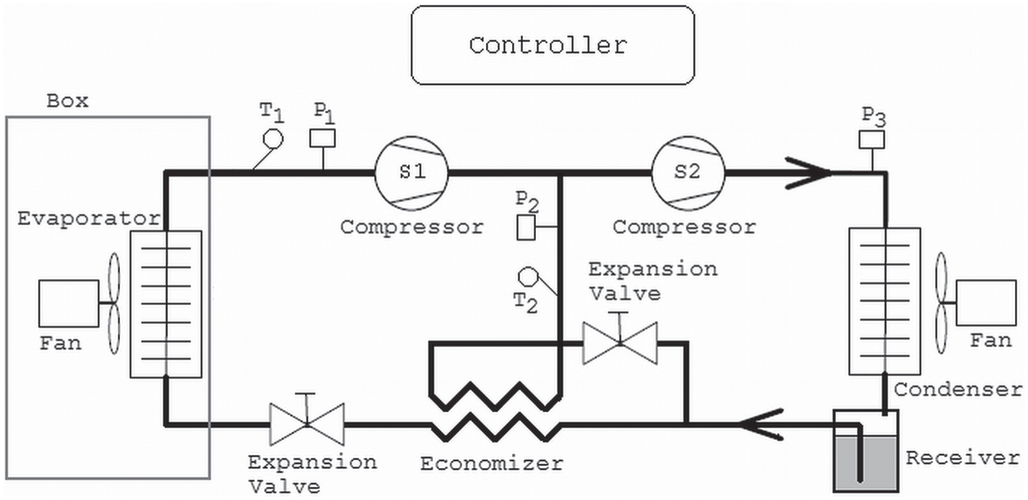
Refrigeration system for the reefer container.
The model has 80 states of which 30 are discrete and 50 are continuous, divided into three discrete and six continuous component models. The model framework is described in the Section 2.2, and the simulation methods are described in Section 2.3.
2.2. Modeling
The model of the refrigeration system is divided into components that each represent a physical component of the system, in other words, a condenser or an evaporator. Each component model is described by two files: an m file that holds the input/output equations of the model and an XML file that describes the properties of the inputs and outputs of the m file. The simulation model is the overall model for the refrigeration plant and its properties are described by an
2.2.1. Component model syntax
Modeling of component models is basically the same as for normal ODE model functions that may be solved by
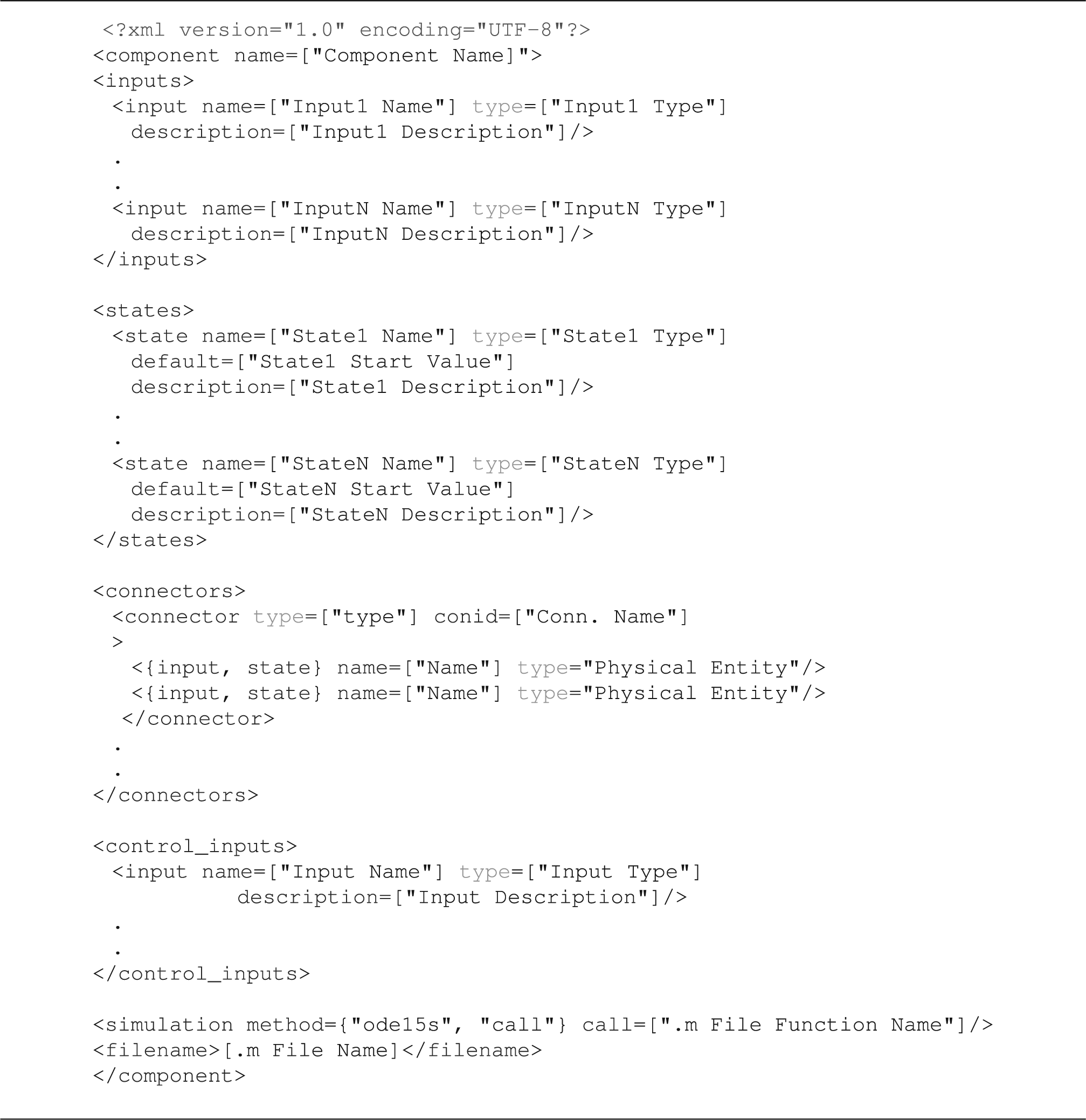
Component model syntax.
The <
Because this environment is used for refrigeration systems, it has a built-in connector class for refrigeration pipe interfaces but obviously, for other applications, other connections will be relevant; see ‘Simulation model syntax’ in Section 2.2.2. On the refrigeration pipe interface three variables exist: a mass flow
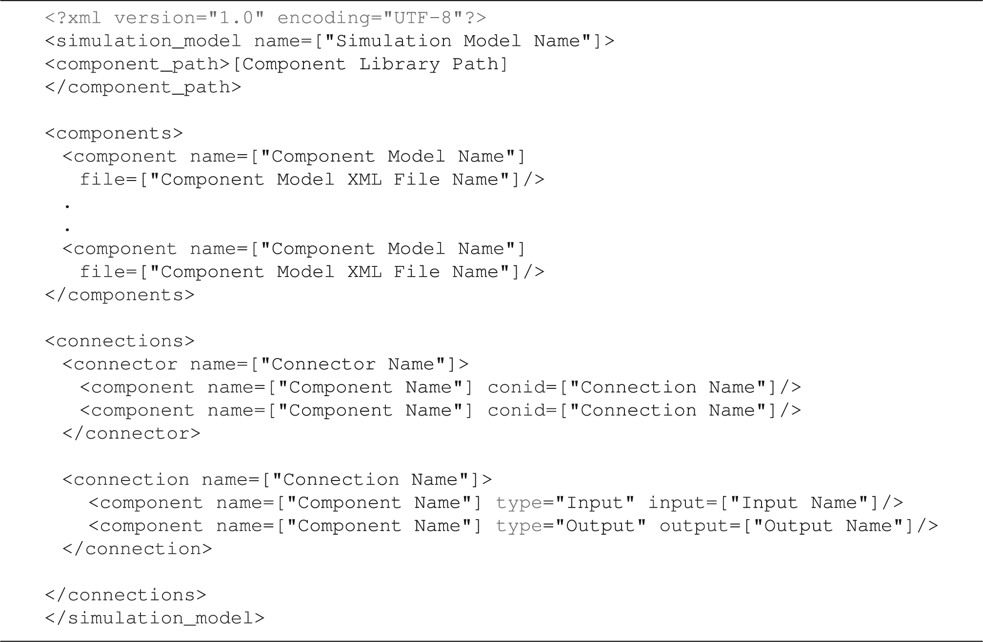
Simulation model syntax.
2.2.2. Simulation model syntax
The syntax for the simulation model XML file is shown in Listing 2.
The simulation model is composed of a set of component models and their connections described by the simulation model XML file, containing a list of the included component models and a description of how the components are connected. The <
The model may be loaded into
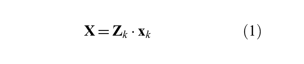
where the index
Because
2.3. Simulation
2.3.1. Multi-rate simulation
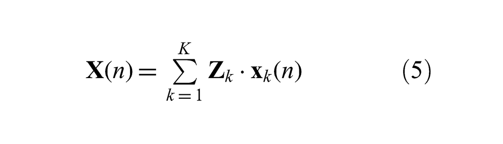
Multi-rate simulation of the system model is done in discrete time steps defined in the time vector given in the simulation function call. In each of the time steps the component models are simulated separately, according to the method defined in the component model XML file, and the results are then combined into the
Example of a simulation model structure.
The discretization of the signals between the component models is equivalent to inserting a ZOH between all models as shown in Figure 2. The inputs to the individual component models are calculated by applying (2) and (3), and given as arguments to the appropriate simulation function such that
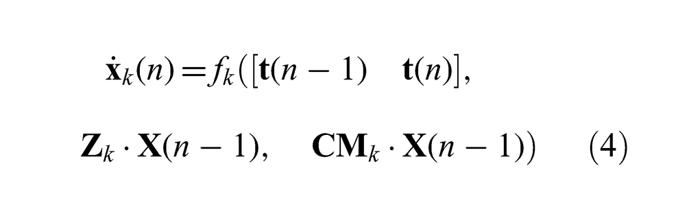
where
where
2.3.2. Monolithic simulation
In a monolithic simulation the entire collection of component models is lumped together by a wrapper function and treated as a single model that may be simulated by ode15s or another solver that accepts functions with a similar interface. This means that for every iteration of the solver all component functions are evaluated in order to find a derivative for the entire collection of component models.
In Sørensen and Stoustrup 18 the multi-rate simulation speed of the reefer container system was compared to the calculated speed for a monolithic simulation of the same system, showing that the modular approach was more than three times faster than the monolithic one. There was no comparison to an actual monolithic simulation of the system but by introducing a monolithic wrapper this is now possible.
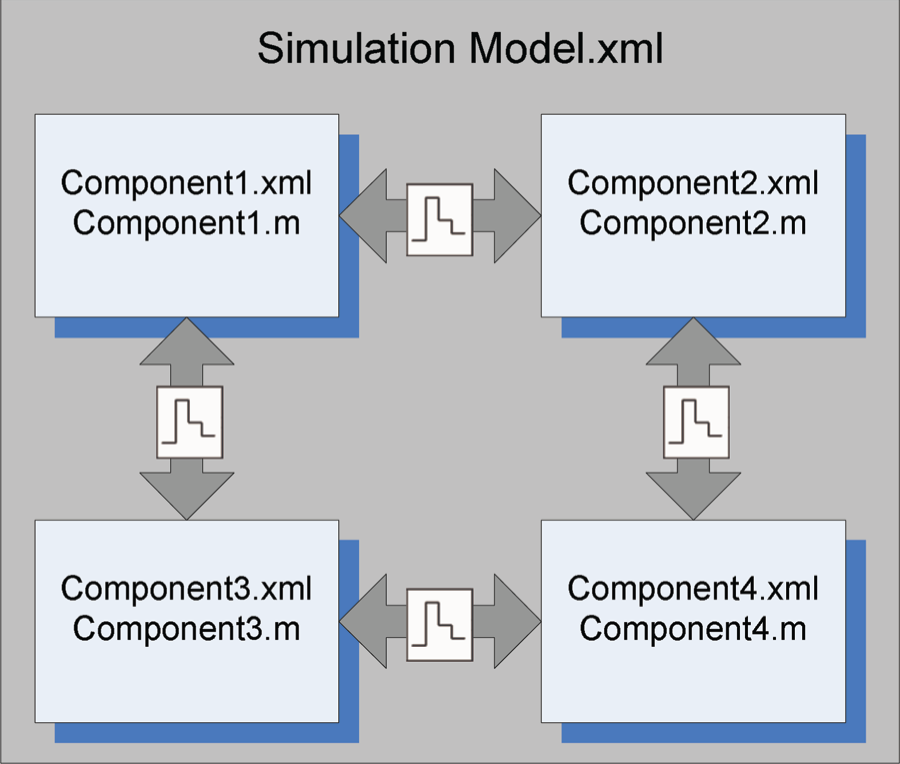
The monolithic wrapper encapsulates the entire model into one function as shown in the example in Figure 3. The function
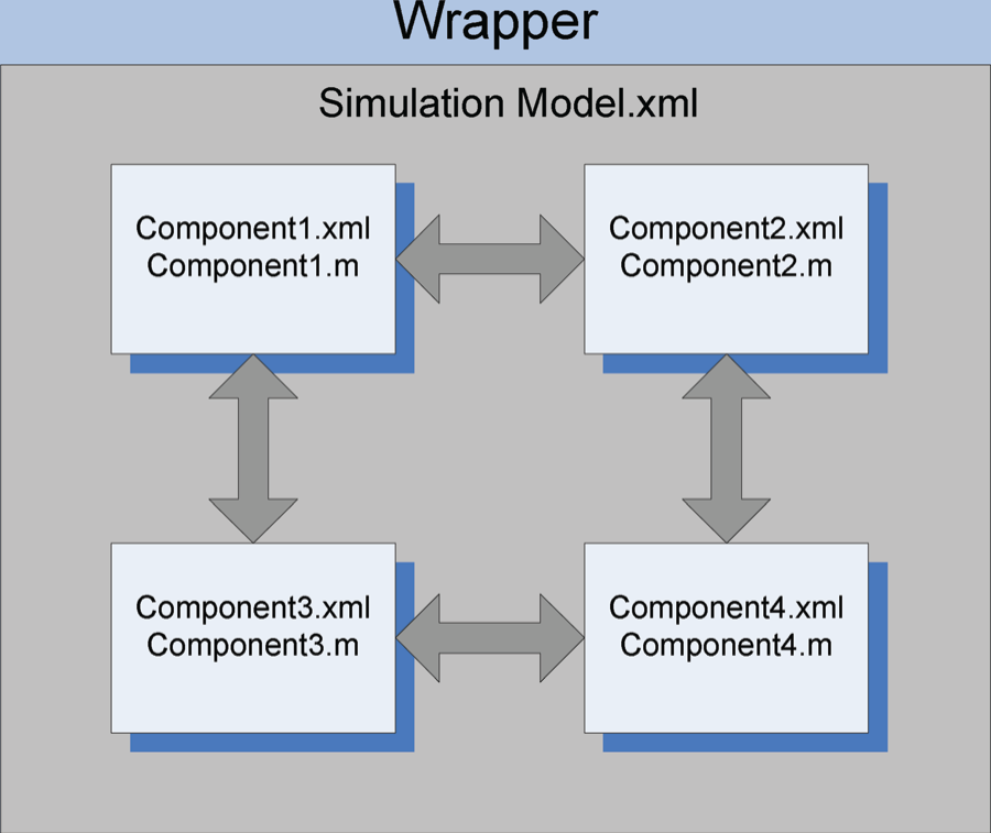
The monolithic wrapper.
In order to achieve a fair comparison to the modular simulation, the monolithic solver’s maximum step size is increased from the default 0.1 s to 1 s such that it can use multiple steps if the dynamics require it, but also run faster if possible. The wrapper will forward results from the ODE and DAE components directly because their output is the state vector gradient, but for the algebraic functions the output is simply the new state at the next sample point and therefore the gradient must be calculated and forwarded to the solver. This is simply the difference between the new and the old state because the algebraic functions of this model are designed for a sample time of 1 s.
2.3.3. Implications of using the ode15s solver
When calling the ode15s solver there is a considerable startup overhead and because the solver is called for each of the continuous components in every discrete time step the total time lost to this is large. According to Shampine and Reichelt 19 the ode15s solver relies on a Jacobian that is generated automatically when it is not supplied by the user, as is the case in this study. Because the calculation of the Jacobian requires a lot of computations the solver only generates the Jacobian when simulation is started, when the order and step size are changed or if the solution is converging too slowly. Another drawback of using the solver in short steps is that it uses a very small step size in the beginning of the simulation period and then gradually increases it. Because the simulation period is so short the solver never reaches larger step sizes and therefore it never reaches the efficiency expected of a variable time step solver, leading to a longer simulation time. In fact, if the model is simulated for 1000 s as a monolithic block by ode15s in one go, the model can be simulated at a speed that is higher than the speed of a multi-rate simulation using ode15s and this shows that a great deal can be gained by using the solver differently, but interaction with the model during simulation is more difficult when the model is simulated in one go by ode15s.
2.3.4. Proposed numerical method
The main goal of the simulation algorithm is to lower the computational burden in order to increase simulation speed and this means that the model should be simulated using as few evaluations of the component model functions as possible and that the startup overhead for the simulation algorithm should be low. The chosen method, a variable-step forward Euler (VS-FE), is the simplest possible and it requires only one evaluation of the component model function per step but it can be unstable if the selected step size is too large.
The stability region for the explicit Euler method consists of the points in the region
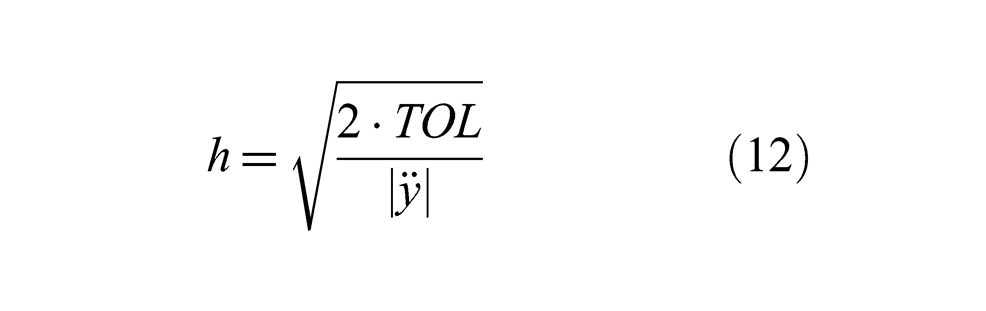
Although the solution converges when using the maximum permissible step size it gives a very inaccurate result because the error is dependent on the step size as shown in (11) and in reality the used step size should be orders of magnitude smaller than the maximum permissible step size in order to ensure a smooth solution.
For higher-order numerical algorithms the local error is found by comparing the results of two different-order calculations and while this requires more calls to the model function and thus increases the computational burden, it also yields better accuracy because an accurate error estimate gives a good step size. Step-size selection algorithms normally compare the local truncation error of the solver with a given fixed tolerance and select the step size such that the local truncation error is smaller than or equal to the tolerance. The method proposed here is an adaptation of a textbook method that is described in Kreyzig
21
and Butcher.
20
The local error
where
where
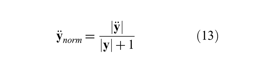
The different types of state in the container model are numerically very different and therefore the second-order derivative is also numerically very different. This means that if the step size is to be determined from the largest second-order derivative given by a model with multiple states the larger states will usually also have the larger second-order derivative. The consequence of this is that states that are small may have a relatively large second-order derivative but it will be ignored and that can result in numerical instability for states of small magnitude. For this model the notion of an absolute error tolerance is therefore impractical and in order to address this problem the second-order derivative is normalized with respect to the size of the states as shown in (13):
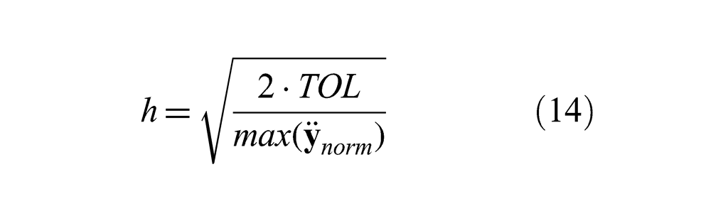
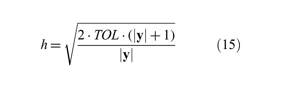
Normalizing the second-order derivative has a drawback: if a state approaches zero the normalized second-order derivative will approach infinity and result in very small steps. This issue is addressed by adding one to the state vector and therefore as a state approaches zero its normalized second-order derivative will approach the real second-order derivative. Due to the normalization of the second-order derivative
In the remaining part of this section the proposed simulation algorithm and its step-size calculation method is described and analyzed, starting with the
2.4. Experiments
The required accuracy for the problem at hand is given by the objectives of the model: it must be adequate for controller experiments and for the model to be used as an observer for FDI in an embedded system. For the controller experiments it is important that the closed loop dynamical behavior of the system is accurate but because the controllers are designed to be robust to a rather large variance in the mechanical system of the containers due to wear and tear and faulty or inadequate maintenance, a maximum error of 2% is acceptable. The average error is the normalized average error on all states and the maximum error is the largest error on any of the states. The errors are calculated from the states of all components except the controller because it will be replaced by an external controller when the model is moved to the embedded system.
When used as an observer for fault detection it is important that the faults are low because a large uncertainty on the simulation result will require higher fault detection thresholds to avoid false positives and thus the ability to detect small faults will be limited or the time to detect a fault will be too long. As an observer the model will be running in open loop and therefore it is important that the long-term static behavior is accurate. A requirement has been chosen that the maximum error on the variables important for control of the system stays below 5% for a three-hour open loop simulation where the control inputs are recorded from a real container.
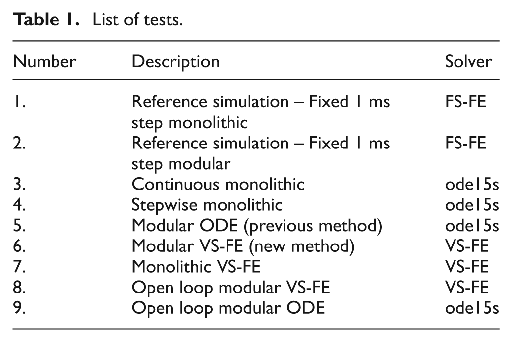
The proposed simulation method is tested in a variety of different scenarios in order to qualify its performance and accuracy in the modes of operation in which it is to be used. Furthermore, a series of experiments are carried out to investigate the ode15s overhead and the nature of the reduction in accuracy caused by the proposed VS-FE method. Table 1 shows a short list of the tests carried out.
List of tests.
In order to calculate the error of the different experiments it is necessary to have a reference simulation that represents the true solution and this is achieved by simulating the model with a fixed step size that is very small compared to the dynamics of the system. In this case a 1 ms step size is found to be adequate by simulating at both 1 ms and 2 ms step sizes and comparing the results, from which it was concluded that the error had converged. Two reference simulations are made: the first test is a monolithic simulation where the model is simulated as one large block at a 1 ms resolution and that represents the true solution without the impact from the ZOH of the modular simulation environment. The second reference is a modular simulation where the components are simulated independently with a 1 ms step size for 1 s at a time and the purpose is to isolate the error introduced by the ZOH between the component models.
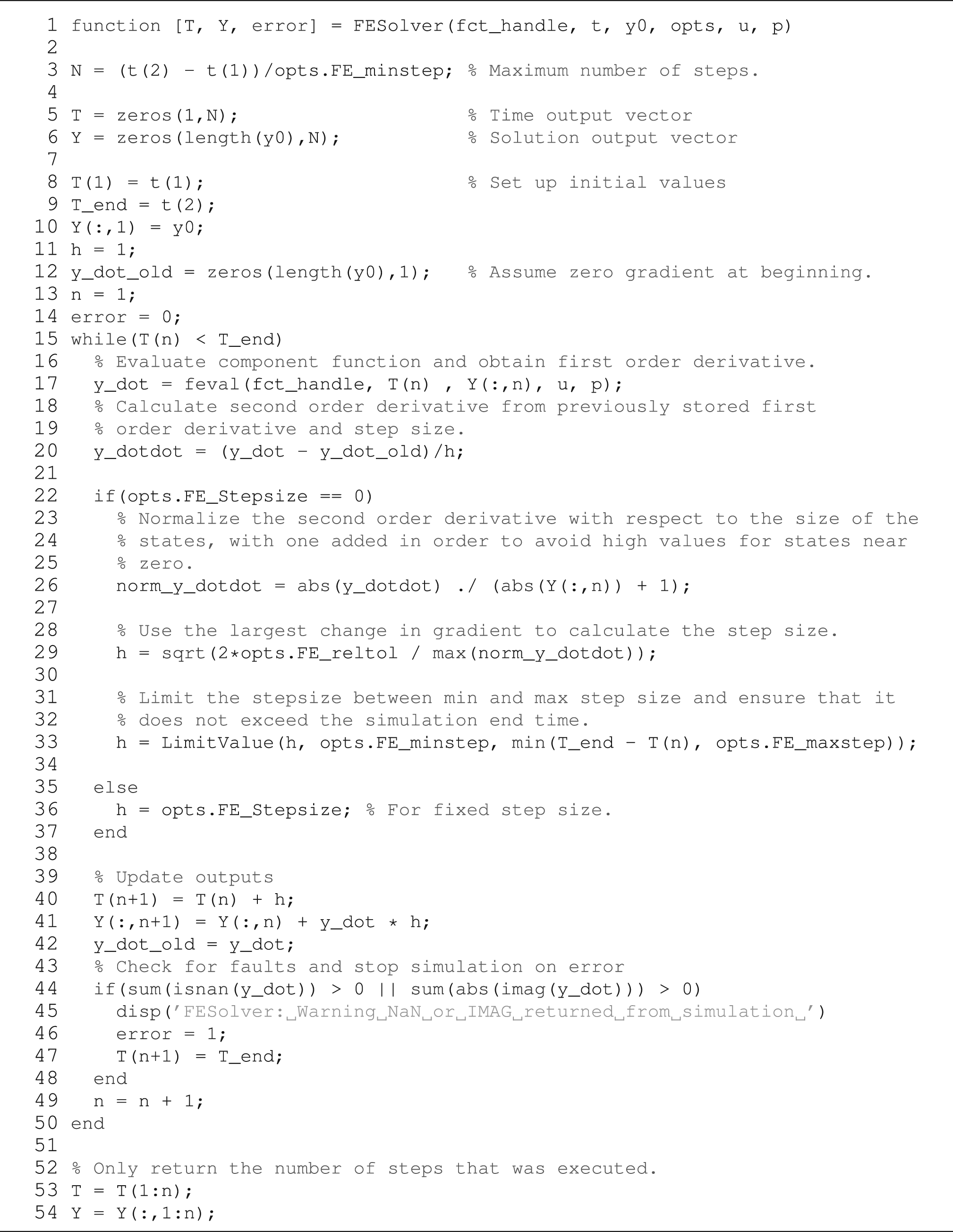
Proposed simulation algorithm.
In these two tests the model is simulated monolithically by the ode15s solver as a sequence of 1 s steps and in one continuous go in order to identify the startup overhead of the solver.
This is the simulation method presented by Sørensen and Stoustrup 18 and it is used as a baseline for verification of the new VS-FE solver.
The VS-FE solver is compared to both reference simulations and to Test 5 in order to verify the performance of the simple solver in a modular environment.
It may be a viable option to simulate the model monolithically in order to avoid any implications from the modular simulation and therefore this test is carried out to verify the speed and accuracy of this solution.
In order to verify the long-term stability and accuracy of the simulation environment the VS-FE solver is used to simulate the system in open loop over a three-hour period with control signals recorded from a real container. The output of the model on the measurements that are important for control of the system is then tested for accuracy by comparing it with sensor measurements from the same real-life data set as the control signals.
The simulation model controller used in this experiment is programmed to ramp the compressor speed nine times during a 1000 s simulation in order to excite the system and create some events that challenge the solver with large gradients on the system states. The modular simulation model that was presented by Sørensen and Stoustrup 18 was not excited as much as in this test, leading to a low error due to the small gradients on the model states. When the system is excited more strongly the state gradients will be higher yielding a larger difference in the zero gradient of the ZOH in the modular environment, which gives a larger error.
3. Results
In this section the results of the tests carried out in Section 2.4 are listed and analyzed in order to identify viable options for simulating the model for controller experiments and for use as an observer on an embedded system. The measured variables are the simulation time, the average error and the maximum error. The average error is the normalized average error on all states and the maximum error is the largest error on any of the states. The errors are calculated from the states of all components except the controller because its states may go to zero and yield an infinite normalized error.
In Figure 4 the main results are shown and the references for calculating the errors are the monolithic reference for the monolithic simulations and the modular reference for the modular simulations. The error tolerance for the VS-FE method has been selected such that the error is approximately the same as that produced by the ode15s solver with standard tolerance settings 19 in order to make comparison of the results easier. From the results in Figure 4 it can be seen that the simple VS-FE solver is able to outperform the more advanced ode15s solver and in the following the reason for this will be analyzed.
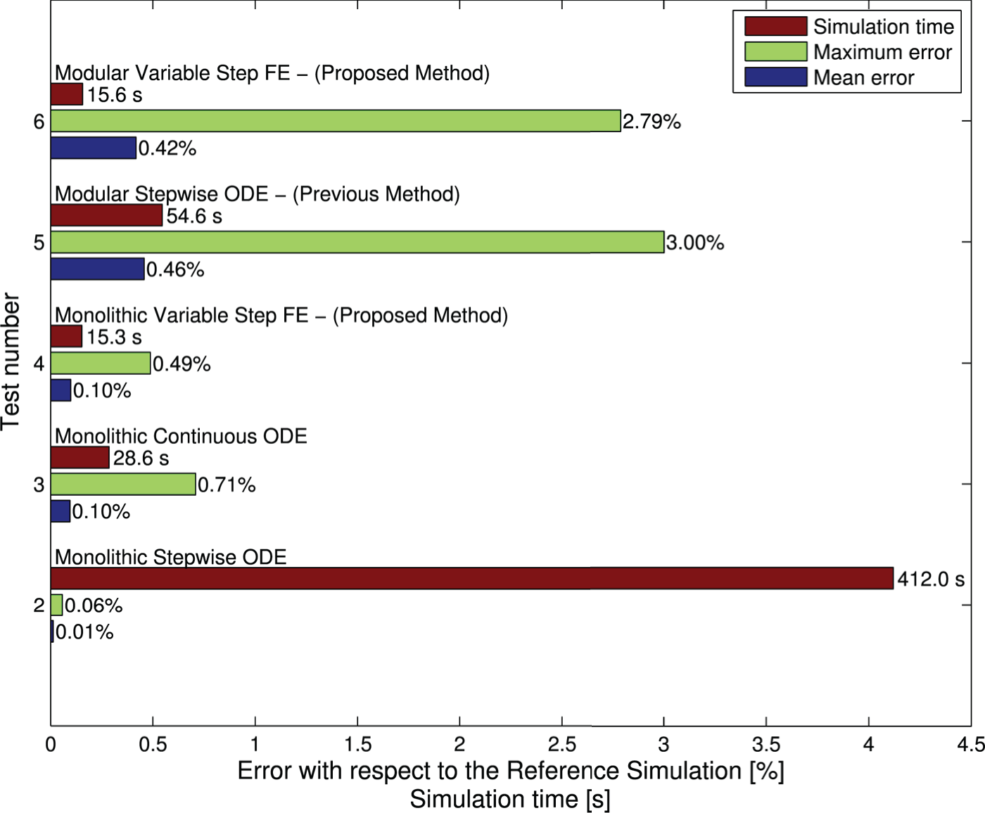
Comparison of test results for monolithic and modular methods.
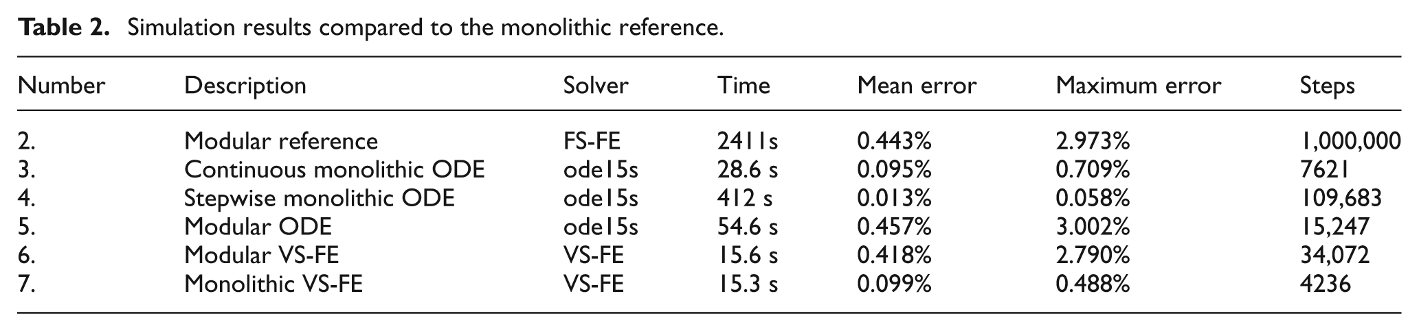
The results of the relevant tests compared to the monolithic reference can be seen in Table 2, where the time column is the time used simulating the 1000 s test and the steps column has the number of steps used by the solver. For modular simulations the number of steps is the sum of steps used on the nine components, and for monolithic simulations it is the number of times the monolithic wrapper function has been called by the solver.
Simulation results compared to the monolithic reference.
The error for Test 2 – Modular reference shows the magnitude of the error introduced from the multi-rate simulation itself and it is a consequence of the ZOH delays between component models. Therefore this error is also large when gradients are as large as they are in this test, due to the high excitation of the model. In a controller experiment setup the ZOH delays are not critical because they are small compared to the dynamics that are important for control, which according to Rasmussen et al. 22 for a refrigeration system are the thermal masses of the evaporator and the condenser. Under normal operation the refrigeration system is in steady state most of the time and therefore the temporal inaccuracy during steep gradients imposed by the ZOH delays has little impact on the accuracy of long-term simulations.
Test 3 – Continuous Monolithic ODE and Test 4 – Stepwise Monolithic ODE illustrate the importance of using the
The results for the old method
18
running on this test sequence are shown in Test 5 – Modular ODE and it can be seen that the error is a bit higher than the error for Test 2 which indicates that
Simulation profile for the modular simulation with the
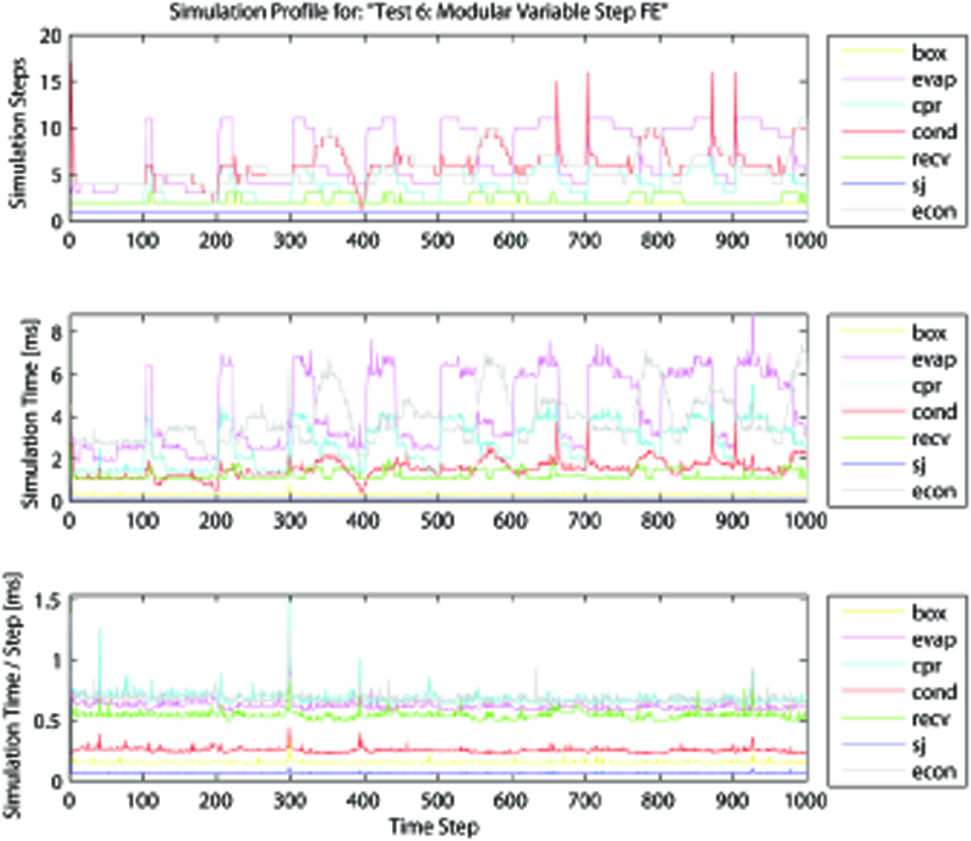
The simple solver shows an unexpected result in Test 6 – Modular VS-FE: it has a shorter simulation time than the old method but it still manages to produce a smaller error than the modular reference simulation. This is because the solver’s crude first-order method causes it to settle faster than the analytical solution and that cancels out some of the error caused by the ZOH in the modular environment. This means that a good comparison of Tests 5 and 6 is difficult when using the monolithic reference and therefore a comparison with the modular reference is also carried out. The simulation profile for this test is shown in Figure 6 and it can be seen that the step size changes more often than for the

Simulation profile for the modular simulation with the VS-FE solver .
From Test 7 – Monolithic VS-FE it can be seen that the VS-FE solver handles the monolithic model quite well. It finishes faster than the continuous monolithic simulation in Test 3 with an error that is roughly the same and it is just as fast as the modular solution which means that using the monolithic simulation method may be one option when there is a need for high accuracy.
Because of the large error from the modular simulators ZOH it is difficult to verify the performance of Tests 5 and 6 and they are therefore compared to the modular reference, with the results shown in Table 3.
Simulation results compared to the modular reference.
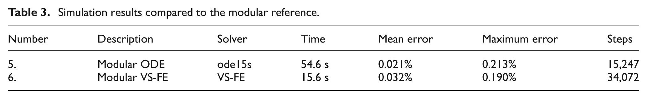
From the results it is clear that the VS-FE solver is capable of simulating this system with the same accuracy as the
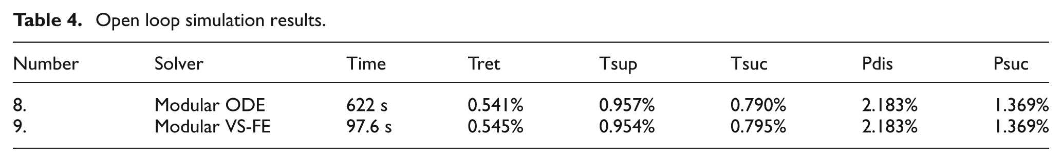
The test sequences in Tests 1 to 7 are designed to show dynamical errors that are relevant when doing controller experiments but they do not verify the long-term stability of the simulation environment and the model. Long-term stability and accuracy are two very important parameters for a simulation model and this is verified with an open loop test that simulates the system model without feedback control for three hours. The initial state for the model is set to match the initial state for a real container and the model is then simulated with the sampled control signals from the refrigeration container. Five measurements that are characteristic for the system are then compared to the results of the simulation in order to verify that the model is stable for longer runs and that the VS-FE solver does not compromise the accuracy of the solution. In Table 4 the results of these two tests are shown. Tret and Tsup are the return and supply air temperatures for the container respectively, and they are important for the temperature control and estimation of actual cooling capacity. The suction temperature Tsuc is the temperature of the refrigerant vapor going from the evaporator to the compressor and combined with the suction pressure Psuc it forms the control signal for control of the evaporator. The last signal Pdis is the discharge pressure of the compressor. With feedback from these five signals it is possible to control the refrigeration system. As can be seen, the errors of the two simulations are almost identical but the VS-FE solver is six times faster than the previous method that uses the
Open loop simulation results.
4. Conclusion
A modular simulation environment was presented with a dynamical model of a refrigeration container. Different options for simulating the model for controller experiments or as a full system observer to be used in the embedded controller for the refrigeration container were tested and analyzed. It was demonstrated that the VS-FE modular simulation approach may be used to simulate vapor compression cycles without the loss of accuracy but with a significant increase in speed. The impact of simulating a model of a refrigeration system with the multi-rate method has been analyzed with respect to dynamical and static errors and it was shown that the multi-rate method combined with the VS-FE solver was the best option for an embedded observer. A comparison between monolithic and multi-rate simulations on the same model was done and showed that the VS-FE solver was faster than the
Footnotes
Funding
This research was funded by the Danish Ministry of Science, Innovation and Higher Education.