






Abstract
This paper aims to develop a CO2 emission model of an acid gas incinerator using Nelder–Mead least squares support vector regression (LS-SVR). The Malaysia Department of Environment is actively imposing the Clean Air Regulation to mandate heavy industries to comply with emission limits. One of the latest measures is to mandate the installation of analytical instrumentation known as a continuous emission monitoring system (CEMS) to report the emission level online to the Department of Environment office. As a hardware-based analyser, CEMS is expensive, maintenance intensive and often unreliable. Therefore, software predictive techniques are often preferred and considered a feasible alternative to replace the CEMS for regulatory compliance. The LS-SVR model is built based on the emissions from an acid gas incinerator that operates in a liquefied natural gas complex. Simulated annealing is first used to determine the initial hyper-parameters, which are further optimized based on the performance of the model using a Nelder–Mead simplex algorithm. The LS-SVR model is shown to outperform a benchmark model based on back-propagation neural networks in both training and testing data.
Introduction
Power plants, chemical plants, government utilities and petroleum refineries typically produce more than the plant’s capacity in order to meet demands. Hence these industries must continuously monitor their exhaust stacks for primary pollutants such as nitrogen oxides, carbon monoxide, sulphur dioxide and carbon dioxide under regulations promulgated under the New Source Performance Standards [US Environmental Protection Agency (EPA) PA 40 CFR Part 60) or the Clean Air Act Amendments Title IV (40 CFR Part 75), 2008] and the Malaysian Environmental Quality Act, 1978 (2000). A continuous emission monitoring system (CEMS) utilizes a sample probe, umbilical and sample conditioning system to extract a representative sample of the stack gas exhaust stream to provide a continuous flow for direct measurement of the pollutant concentration on individual analysers (Fan and Zheng, 2009). A data acquisition system (DAS) is typically used to collect, calculate emission rates, alarm and store historical data from these CEMS (Zheng and Tang, 2008). The promulgated regulations in US EPA 40 CFR covering the monitoring of combustion units for primary and other pollutants allow for the use of predictive emissions monitoring systems (PEMS) in lieu of CEMS. A PEMS is a sophisticated software-based sensor/prediction system that is directly interfaced with the process control system and inputs from the combustion or pollution control process. The US EPA (2011) have revealed the devastating effects of the continuous release of pollutants such as carbon dioxide, methane, nitrous dioxide and other greenhouse (heat-trapping) gases into the atmosphere. Climate change induced by these gases can cause damage to human health, agriculture, natural ecosystems, coastal areas and other climate sensitive systems. Currently, emission monitoring is done via analytical instruments, which are very expensive to install and maintain; the cost for an online NOx analytical and monitoring system is around $100,000–200,000 and the cost for maintenance is approximately $15,000 per year (Dong and McAvoy, 1995). Several studies have been performed to develop predictive systems for industrial emissions. One of the earlier ideas was presented by Baines (1999), a consultant from Fisher-Rosemount Solutions. The author proposed the idea of predicting the stack contaminants in real time by correlating emissions with key unit parameters like fuel type, air and fuel flows, and combustion temperature. Chakravarthy et al. (2000) have developed a PEMS for industrial process heaters. The authors have used heuristic an optimizer genetic algorithm (GA) to tune the NOx kinetic parameters. Deng and Stobart (2007) examined the idea of using a hybrid clustering technique that involves the modifications of the Fuzzy C-means method and using neural networks to achieve the best performance of the fuzzy system for a diesel engine emission model. Zheng et al. (2008) used a generalized regression neural network (GRNN) to establish a non-linear model between the parameters of the boiler (of 300 MW steam capacity) and the NOx emissions. Later, the same authors have proposed the idea of replacing the existing GRNN PEMS with a least squares support vector regression (LS-SVR) model. The authors claim that this new algorithm yields better accuracy of a coal combustion unit (Zheng et al., 2010). The main objective of this paper is to develop a CO2 emission model of an acid gas incinerator based on an LS-SVR algorithm with Nelder–Mead (NM) optimization of its hyper-parameters. This paper is organized as follows: Section 2 presents a brief literature on artificial neural networks (ANNs) and LS-SVR. Section 3 describes the modelling background in terms of the parameters used, a case study of an acid gas incinerator and the dataset used. Section 4 presents the results and analysis, and Section 5 gives a brief conclusion.
Literature review
Artificial neural network (ANN)
An ANN is represented as non-linear interconnected layers of processing nodes, which are normally referred to as neurons, a term borrowed from neurobiology (Zhou et al., 2004). The most common class of ANN is the multilayered feedforward network, which primarily consists of an input layer, one or more hidden layers and an output layer. The input layer holds the data and distributes it to the network via interconnections (neurons) in the hidden layer(s), where they are processed by the activation function to produce an output signal. This type of network is also known as a multilayer perceptron (MLP) (Haykins, 1999); a typical MLP network is shown in Figure 1. Common transfer functions used are linear, log-sigmoid, and tan-sigmoid as shown in Equations (1), (2) and (3).
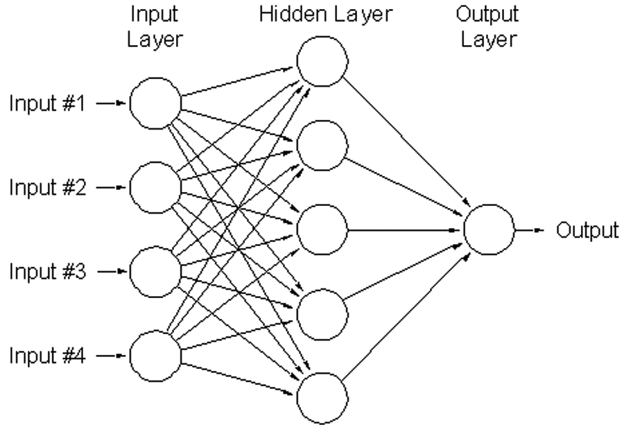
Typical feedforward back-propagation network.
where A is the element activation function and is represented by Equation (4):
The variable
Support vector regression (SVR)
The foundations of support vector machines (SVM) were laid by Vapnik (1995). Early SVMs were developed for classification problems; later they were extended to the domain of regression problems (Vapnik et al., 1997) and collectively known as support vector regression (SVR). The formulation for SVR begins with a set of data (Gunn, 1998):
which is to be approximated to a non-linear function:
Where
Where
Using an
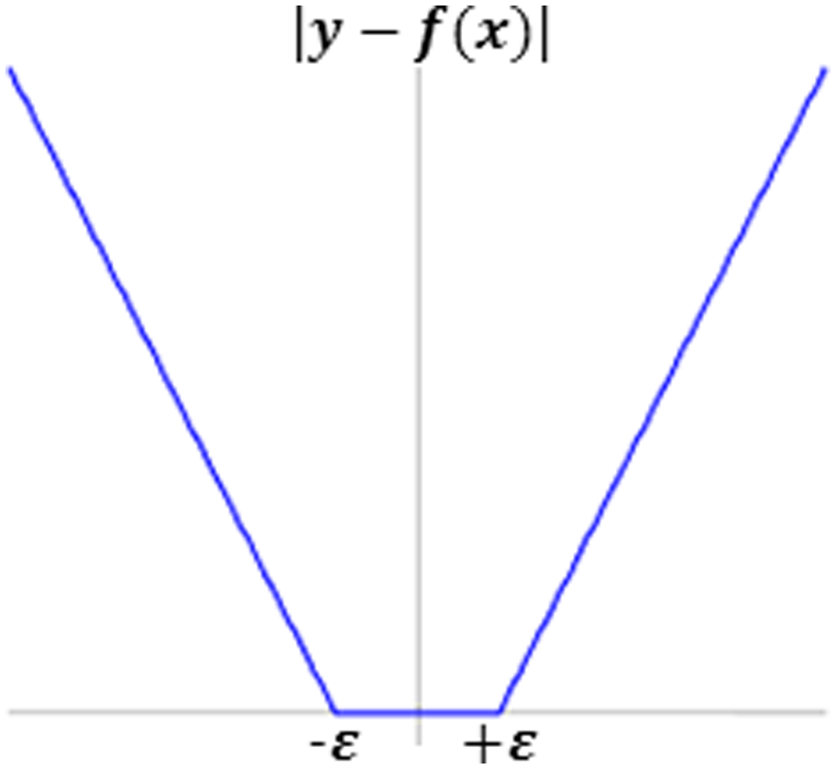
Employing the Lagrangian duality theorem, the minimization problem becomes:
With constraints
Solving Equations (9) and (10) determines the Lagrange multipliers,
where
Least squares support vector regression (LS-SVR)
The SVM formulation above leads to a QP problem with linear constraints. The size of the matrix involved in the QP problem is directly proportional to the size of the training data (Zheng et al., 2010). To reduce the complexity of the optimization problem, Suykens et al. (2002) introduced a modified version of the SVM called the least squares SVM (LS-SVM). This formulation results in a set of linear equations instead of a QP problem. The LS-SVM is used for both classification and regression problems. The formulation for LS-SVR is begun by taking a training set as in Equation (5) and estimate using a non-linear function as in Equation (6) where
Subject to:
The optimization formulation in Equation (13) is a ridge regression cost function formulated in feature space. Constructing the Lagrangian of the problem, the dual problem is derived:
The conditions for optimality are given by (Suykens et al., 2002):
Upon elimination of the variables
Where
Hence the resulting LS-SVR model becomes:
In this paper, a radial basis function (RBF) kernel function is used:
Where
Modelling background
Back-propagation neural network (BPNN) model
Two models will be developed in this paper using two distinctive algorithms. The first model is developed as a benchmark using a BPNN. The optimal network parameters are chosen by varying the number of layers and the number of hidden neurons per layer. The parameter that gives the best performance is chosen and shown below:
Number of layers=2;
Number of neurons (hidden layer)=20;
Transfer functions (input layer)=tan-sigmoid;
Transfer function (hidden layer)=linear;
Training algorithm=Levenberg–Marquardt.
Nelder–Mead (NM) least squares support vector regression (LS-SVR)
It is understood that the hyper-parameters involved for the standard SVM with RBF kernel are
Expansion steps=2;
Size of initial simplex=1.2;
Contraction steps=0.5;
Reflection steps=1;
Shrinkage steps=0.5;
Number of optimization steps=15;
Number of function evaluations=50;
Stopping criterion based on value of function=1e-6;
Stopping criterion based on change in minimizer=1e-6.
The initial values of the hyper-parameters (
Initial temperature=1;
Max number of function evaluations=40;
Number of steps at fixed temperature=20;
Energy tolerance=1e-45.
Using SA alone is not very strong because of the stopping criterion (i.e. number of iterations). The combination of SA and NM is much stronger. SA is only used as a ‘cost effective’ method for locating the initial hyper-parameters. The performances of the models are gauged using standard performance functions in the form of correlation factor (R), root mean square error (RMSE) and accuracy.
Where
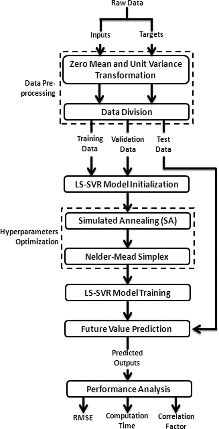
Nelder–Mead least squares support vector regression (LS-SVR) flowchart. RMSE, root mean square error.
Case study
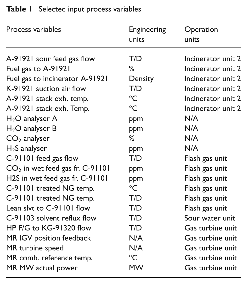
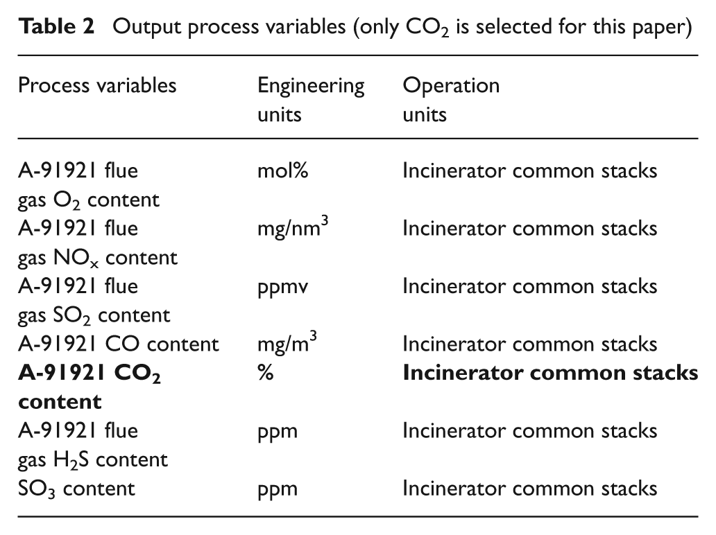
In this paper, the CO2 emission from a tangentially fired acid gas incinerator is modelled. This incinerator train is part of a liquefied natural gas (LNG) complex. The plant is divided into four sections consisting of upstream facilities, gas treating, liquefaction and storage/terminal. The first part of the gas treating section deals with the acid gas in the feed. CO2 and H2S are removed to meet product specification. An amine-based solvent is used in the acid gas removal process. Solvents with absorbed acid gases are regenerated in regenerator column at high temperature and low pressure. The acid gases are then incinerated before being discharged safely into the environment. In this LNG complex, acid gases are incinerated using two methods: one uses steam boilers and the other uses acid gas thermal incinerators (Jamaludin et al., 2005). The process flow scheme of the incinerator train is shown in Figure 4. The main constituents of the inputs to the incinerator are acid gas, flash gas, fuel gas and combustion air. The flue gases that are released into the stack consist of NOx, SO2, SO3, CO, CO2 and H2S. In this paper, only CO2 emission will be modelled based on the plant input and output process variable data. The data is obtained from the LNG complex incinerator train distributed control system historical dataset taken from April 2010 to November 2010, and contains the data from 29 input process variables and seven output process variables. The most relevant process variables are selected by reviewing the design and operational specifications in the incinerator material balance sheet. An initial correlation analysis was also performed to the dataset to determine the variables that have the strongest variance with each other.
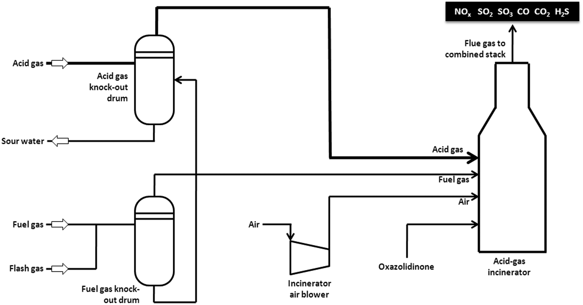
Process flow scheme of incinerator train.
As a result, 22 input variables and one output variable (i.e. flue gas CO2 content) are chosen with 1044 samples, taken at 30 minutes apart for the whole month of September 2010. The number of data points for LS-SVR is limited by the computational ability of the machine that is used to run the model, mainly because the M-file implementation is memory intensive compared with C-Mex or C++ languages. Tables 1 and 2 outline the characteristics of the chosen input and output variables. The relationship between CO2 and the input variables are not easily modelled mathematically (and it is beyond the scope of this paper) and any attempt on graphical plotting shows erratic distributions (which on some level demonstrates a highly non-linear relationship).
Selected input process variables
Output process variables (only CO2 is selected for this paper)
However, the relationship can be proven by correlation analysis and by studying the process flow and material balance of the feed and product gases. Before modelling, data is pre-processed to remove bad inputs and non-values. For ANN modelling, 70% of samples are used for training, 15% for validation and 15% for testing; the SVR model uses 80% for training and cross-validation, and 20% for testing.
Results and analysis
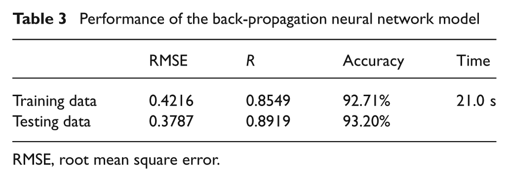
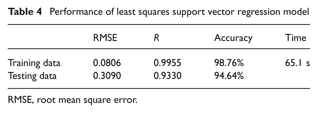
The individual model performance of BPNN and LS-SVR will be presented in this section. Tables 3 and 4 presents a comparison of the performance of the models in terms of correlation, root means squared and accuracy of the predicted values. The performance of both models in terms of computational time is also shown. Figures 5, 6, 7 and 8 show distribution of real and predicted results. This will be followed by a brief analysis of the results obtained. The performance of the LS-SVR model depends greatly upon the values of the hyper-parameters selected. The initial values for the hyper-parameters are:
Performance of the back-propagation neural network model
RMSE, root mean square error.
Performance of least squares support vector regression model
RMSE, root mean square error.
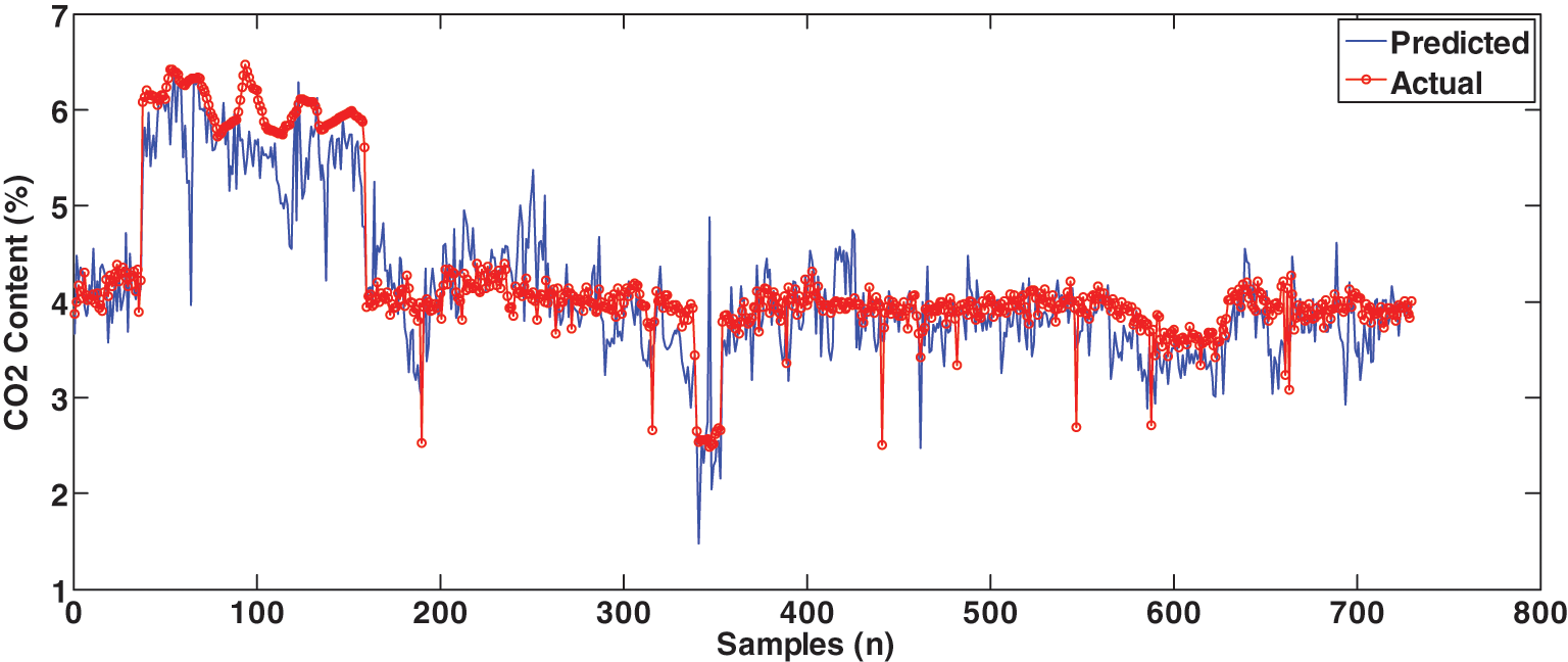
CO2 training data for back-propagation neural network.
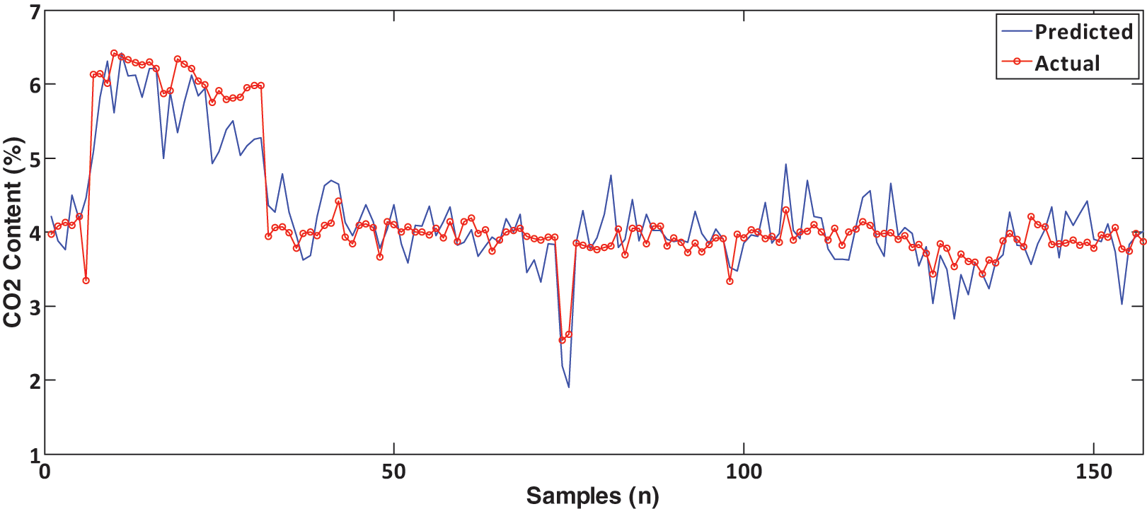
CO2 testing data for back-propagation neural network.
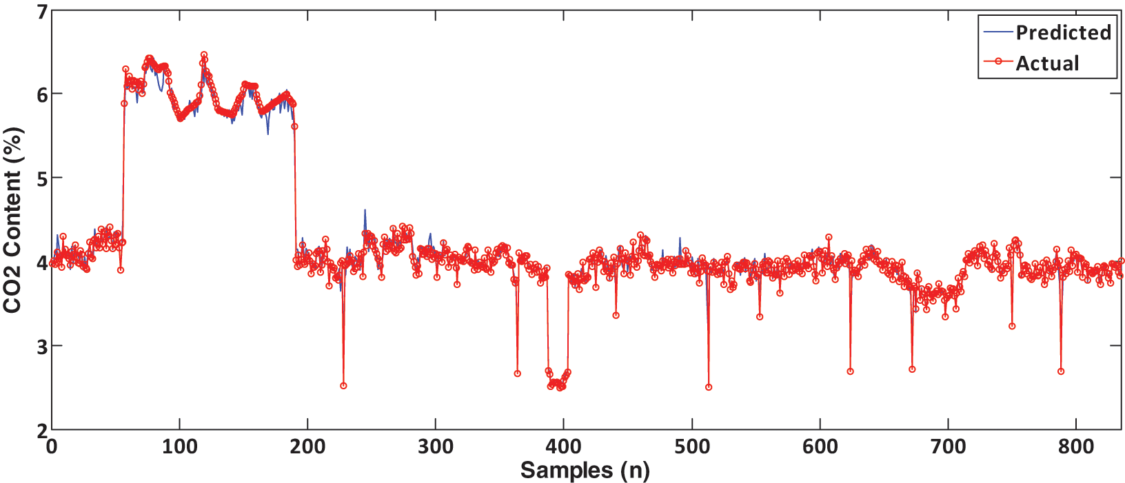
CO2 training data for least squares support vector regression.
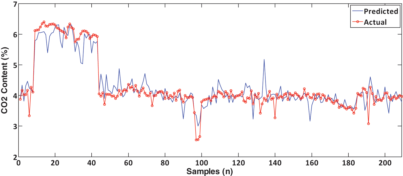
CO2 testing data for least squares support vector regression.
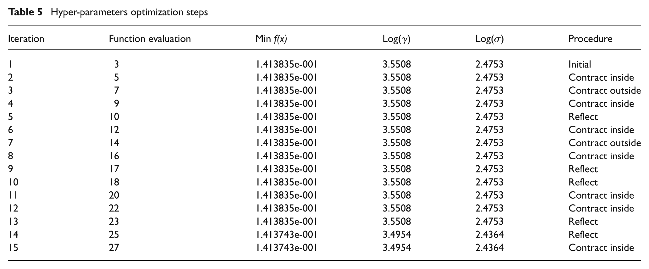
Hyper-parameters optimization steps
The CO2 emission as shown in the above graphs presents a highly non-linear distribution; hence it takes a model with the capabilities to map these non-linearities with precision and accuracy. As shown in Tables 3 and 4, the performance of the LS-SVR model is clearly superior in both training and testing data compared with the BPNN model. The graphs also show that the LS-SVR model is able to track and predict the CO2 emission with much better accuracy than BPNN model. The accuracy achieved by both models is above 90%, which satisfies the conditions under the US EPA Performance Specification 16 for Predictive Emission Monitoring Systems (2008). The models developed can be used in real world applications. LS-SVR is a much more ‘transparent’ algorithm, where the resultant model has weights and biases that were optimized to suit the particular dataset. Another plausible explanation is that, with BPNN, the initial weights are chosen randomly and hence the performance varies significantly with the number of simulations as shown by Zheng et al. (2008). In contrast, LS-SVR initial parameters are optimized via SA. The solutions provided by SVMs are unique and global in a dual space problem; this is achieved by solving the Karush–Kuhn Tucker (KKT) system at its core. The generalization ability of LS-SVM could be further improved by increasing the number of samples used for validation and reducing the stopping criteria when training using cross-validation. SVM algorithms are a kernel-based method; hence the complexity is in the order of
The LS-SVR solution comes from solving the linear system in Equation (16) by matrix inversion; this is a fairly tedious process to be solved numerically and results in a longer overall computation time, as shown in Table 4. Hence, the usability of LS-SVR depends heavily upon the number of samples used and the processing power of the machine that it currently runs on. To overcome this, several fixes have been proposed such as using quadratic Renyi entropy to select the most significant support vectors (Jiang et al., 2008), sequential learning LS-SVM (Jung and Polani, 2008), and using analytic QP and sparseness (Platt, 1999). One of the weaknesses of the NM optimizer as shown in Table 5 is that it only searches one better point (i.e. min f(x)=1.413743 e-001) in 15 iterations. This could be improved by increasing the expansion sizes that includes the contraction, reflection and shrinkage. In the future, a more complex optimizer will be considered to perform the hyper-parameters optimization. In Table 3, it can be seen that the testing performance of BPNN is better than training, which shows a good generalization ability, but to reduce overgeneralization, the number of training samples could be improved, while reducing validation and testing samples.
Conclusion and recommendations
In a nutshell, this paper has brought into focus the ability to model the CO2 emission from an acid gas incinerator using an NM LS-SVR algorithm. The modelling was done using a series of steps that includes optimizing initial hyper-parameters and further optimization using a NM simplex algorithm. As a result, the LS-SVR model performs significantly better for both training and testing data compared with the benchmark BPNN model.
Additionally, the ability to track and predict future values of CO2 emission with remarkable accuracy has also been demonstrated by the LS-SVR model. The superiority of the LS-SVR model can be accounted for by the ability to reach a global and unique solution for the minimization of a convex function. The proposed algorithm is robust in terms of the class of the problem that it can handle, be it classification or complex regression with multiple dimensions. However, one of the drawbacks of LS-SVR includes heavy computational dependencies when it comes to large datasets. Nevertheless, this could be improved using newer techniques. Overall, the primary objective of the paper has been achieved, and in the future, a hybrid model that involves SVMs with complex optimization will be developed in order to improve further the predictive accuracy and computational efficiencies.
Footnotes
Funding
This research received no specific grant from any funding agency in the public, commercial, or not-for-profit sectors.