In this paper, the design methods of decentralized PID controllers based on decoupled subsystems are proposed for two-input two-output systems. The higher-order decoupled subsystems are reduced into simple dynamics such as first-order plus dead-time or second-order plus dead-time and the dominant poles are placed at desired locations. The well tuned parameters of decentralized PID controllers can be obtained based on the movement of poles to get the desired closed-loop response of the system. A corollary derived from the generalized Nyquist stability theorem is used to ascertain the nominal system stability and to hold robust stability in the presence of the process multiplicative uncertainties. Finally, two simulation examples are provided for the validity and effectiveness of the proposed design methods. It can be observed that the high closed-loop performance is obtained using the proposed methods and it is comparable to recent methods available in the literature.
In chemical process industry, two-input two-output (TITO) processes are frequently encountered multivariable processes, and moreover, a large number of multivariable processes with inputs/outputs beyond two can be treated as several two-by-two subsystems in engineering practice (Lengare et al., 2012; Liu et al., 2005, 2006). The general solution to multivariable control system design and tuning can be based on model-predictive control (Åström et al., 2002; Jevtović and Mataušek, 2010; Nordfeldt and Hägglund, 2006). However, this control is used today on a higher level, to give set-points for PI/PID controllers preferred in lower-level loops. The improvement of performance is actually due to improvements in the lower-level PID loops. The improvement at the lower level can be obtained in the following two ways. One way is to find an effective design method for decentralized single-input single-output (SISO) control (Gundes et al., 2009), and other is to use a decoupler: static (Åström et al., 2002; Lee et al., 2005) or dynamic (Goodwin et al., 2001; Huang and Lin, 2006; Nordfeldt and Hägglund, 2006; Tavakoli et al., 2006). Despite the development of advanced multivariable or centralized controllers, the multiloop or decentralized PI/PID control using multiple SISO PI/PID controllers remains the standard for controlling multi-input multi-output (MIMO) systems with modest interaction (Campo et al., 1994; Lee et al., 1998; Vu and Lee, 2010). However, due to process and loop interactions, the design and tuning of multiloop controllers is much more difficult compared to that of single-loop controllers. Since the controllers interact with each other, the tuning of one loop cannot be done independently. Applying the tuning methods for SISO systems to multiloop systems often leads to poor performance and stability. Much research has been focused on how to efficiently take loop interactions into account in multiloop controller design (Vu and Lee, 2010).
In the literature, many methods have been presented for multiloop controller design including the detuning method (Chien et al., 1998; Luyben and Jutan, 1986), sequential loop closing (SLC) method (Bao et al., 1999; Lee et al., 2003), relay auto-tuning method (Åström and Hägglund, 1988; Halevi et al., 1997; Loh et al., 1993; Shen and Yu, 1994; Tan and Ferdous, 2003) and independent loop method (Hovd and Skogestad, 1993; Lee et al., 1998; Wang et al., 1998). Some of the decentralized methods found in literature could be classified under the following topics. A common way is first to design an individual controller for each control loop by ignoring all interactions and then to detune each loop by a detuning factor. The biggest log modulus tuning (BLT) method is a typical example of the detuning method, presented by Luyben and Jutan (1986). Similar methods have also been addressed by Chien et al. (1998). The detuning methods are simple, but the loop performance and stability of the system cannot be clearly defined through the detuning procedures. In the sequential design method, by taking interactions from the closed loops into account in a sequential fashion, multiple single-loop design strategies can be directly employed (Hovd and Skogestad, 1994; Shiu and Huang, 1998). Lee et al. (2003) suggested a multiloop controller design method by considering the frequency-dependent properties of the closed-loop interactions and internal model control (IMC)-PID tuning rule for SISO systems. Bao et al. (1999) formulated the multiloop design as a nonlinear optimization problem with matrix inequality constraints. In the sequential design method, the loops are usually closed from the fastest loop, one after the other. However, the final controller design may depend on the order in which the controllers are designed, and iteration procedures are essential because closing the subsequent loops may alter the response of the previously designed loops (Skogestad and Morari, 1989). In the relay auto-tuning method, the relay-feedback technique is applied to the design of each corresponding SISO controller (Åström and Hägglund, 1988). The control loops are tuned sequentially and the multiloop control system is designed in a sequence of SISO design problems. These methods consider the interaction in a sequential manner, require minimum process information, but tuning sequence has to be repeated. In recent years, independent design methods have been presented by several authors, in which each controller is designed based on the paired transfer functions, satisfying some constraints due to the loop interaction (Hovd and Skogestad, 1993). To decide the constraints for the individual loops, criteria such as interaction measure and Gershgorin bands are used (Chen and Seborg, 2003). Lee et al. (1998) proposed the trial-and-error method to design decentralized PI controller tuning. Wang et al. (1998) used a modified Ziegler–Nichols method to determine controller parameters to achieve a specified gain margin. In these methods, as detailed information about the controller dynamics in other loops is not used, the resulting performance may be poor (Hovd and Skogestad, 1994).
In this paper, a simple decoupler plus a decentralized PID controller is proposed for TITO systems based on pole placement approach. However, an arbitrary pole placement is difficult to achieve for higher-order or time-delay systems by low-order feedback controllers such as PID. To overcome this difficulty, in the proposed work the dominant pole placement method is used to design decentralized PID control (Mokadam et al., 2013; Wang et al., 2009).
The paper is organized as follows. In section ‘The decoupler design method’, the decoupler design method is presented. A decoupled diagonal higher-order model is reduced to equivalent first-order plus dead-time (FOPDT) and second-order plus dead-time (SOPDT) models in section ‘Model reduction’. The proposed PID controller design methods for FOPDT and SOPDT models are addressed in section ‘Controller design method’. In section ‘Stability analysis multiloop system’, the sufficient and necessary conditions for tuning the adjustable parameters of proposed multiloop controllers to hold nominal and robust stability are discussed. Two simulation examples are given in section ‘Simulation study’. The conclusions are summarized in the conclusion section.
Control scheme for TITO systems
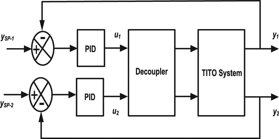
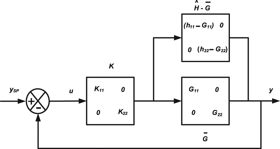
The work presented in this paper is focused on TITO systems.The structure depicted in Figure 1 is sometimes used for the control of TITO systems (Nordfeldt and Hägglund, 2006). In this control structure, two PID controllers, that take the two measurement signals as inputs, are used. The output signals from the PID controllers enter a decoupler, and the outputs from the decoupler form the two inputs to the process. Hence the control problem is separated into two parts, one part that deals with decoupling and a second part that concerns control of decoupled loops. The main contribution of this paper is that it provides such methods.
Block diagram of the proposed control structure for a TITO system.
The decoupler design method
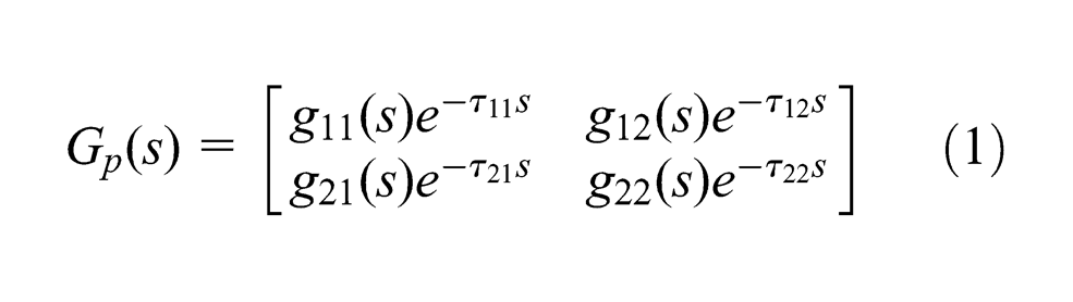
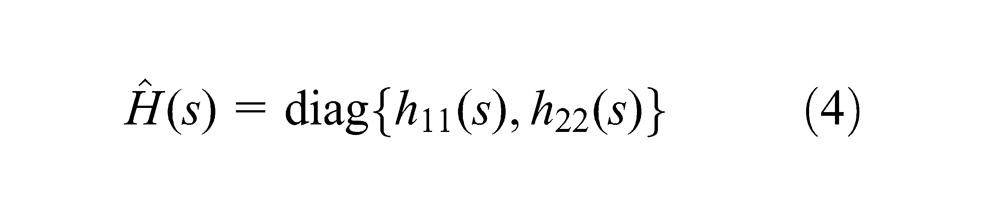
Consider a FOPDT TITO process with transfer function matrix
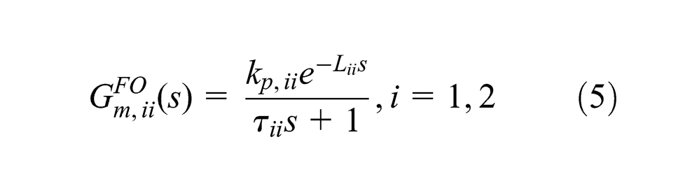
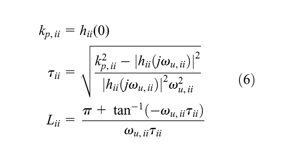
Three unknown parameters (, and ) in equation (5) need to be determined, in order to obtain the FOPDT model of . In this paper, the FOPDT model is obtained based on frequency response fitting at two points, and , where is the phase crossover frequency (Wang et al., 2003). As a result, the parameters of the FOPDT model can be obtained as follows:
SOPDT model reduction
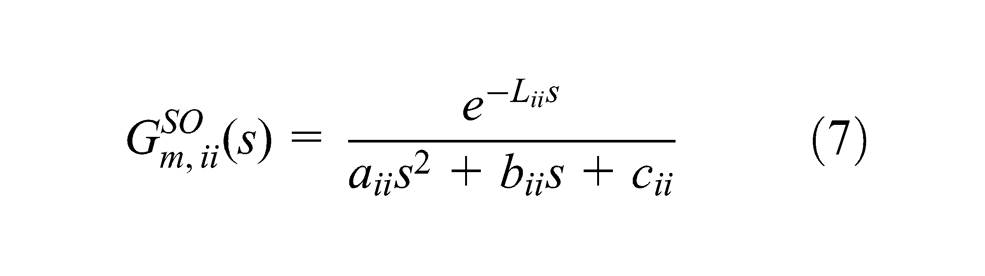
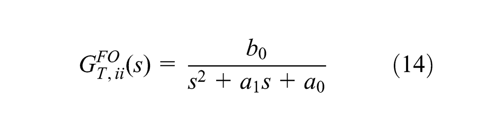
If industrial systems have an oscillatory step response, a FOPDT model cannot include complete dynamics. SOPDT models are commonly preferred for systems which have underdamped, critically damped and overdamped dynamics (Panda et al., 2004). For this reason the SOPDT model in the form
is used.
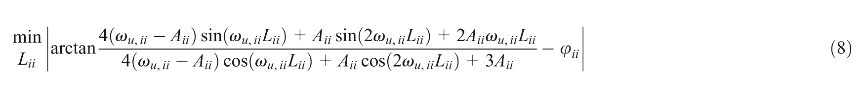
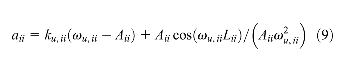
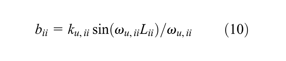
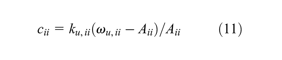
To find an approximate SOPDT model for each element of , four unknown parameters (, , and ) in equation (7) need to be determined. Based on the tangent rule, the SOPDT model is determined using the following relations (Šekara and Mataušek, 2010):
where
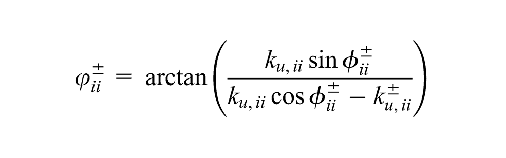
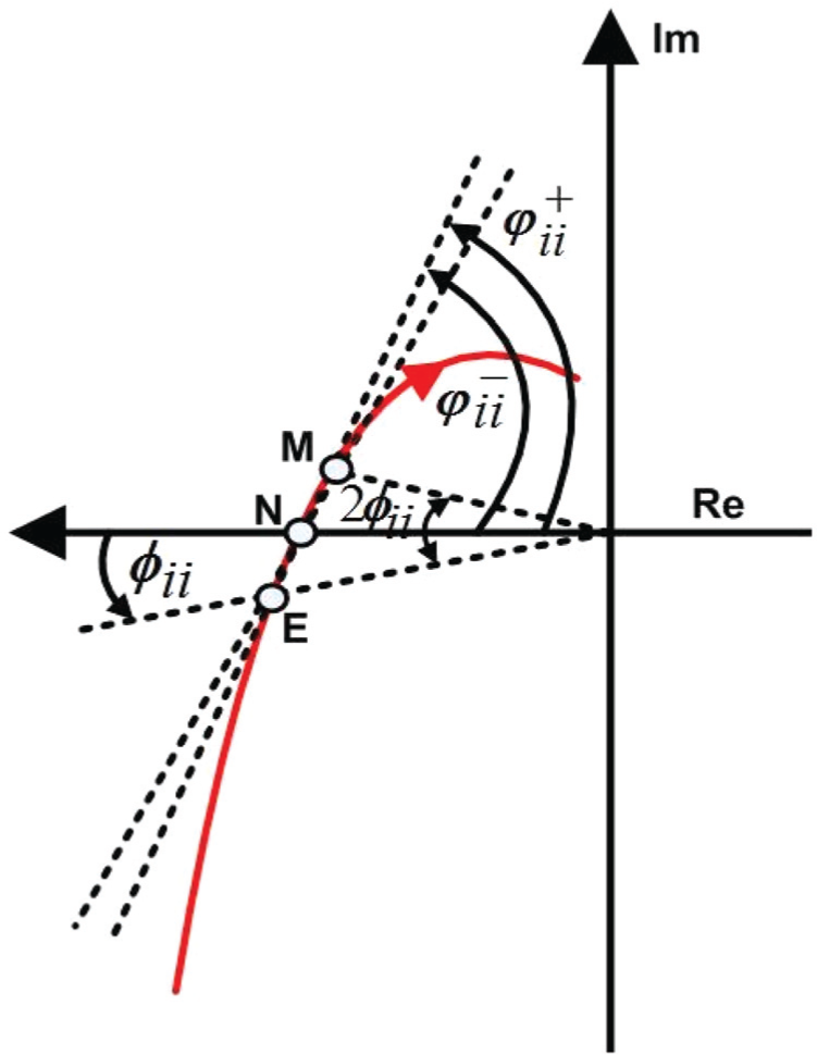
and the parameter is the angle of the tangent to the Nyquist curve of each element of at the ultimate point . Here and are the ultimate gain and the ultimate frequency respectively.
The graphical procedure to find an angle from the Nyquist curve of each element of is presented as follows. Consider the three points , and on the Nyquist curve of as shown in Figure 2. The angle is obtained as the mean value , where
Estimation of the angle from the Nyquist curve of
Controller design method
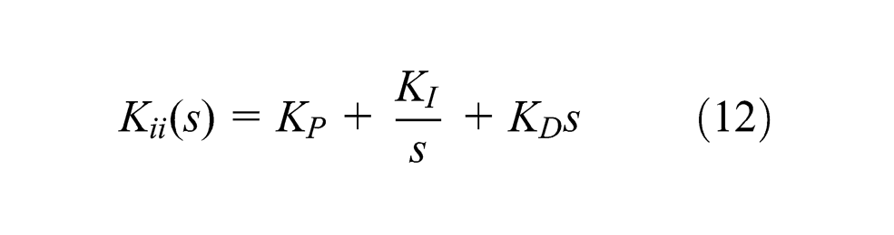
A decentralized PID controller is used to control the TITO system . The structure of each PID controller is
PID design method for FOPDT systems
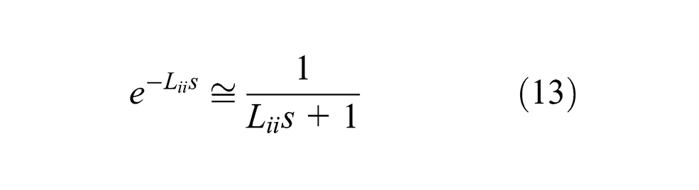
Consider a FOPDT model of the decoupled system given in equation (5). The dead-time can be approximated using a first-order Pade or first-order Taylor series approximation. In this paper, a first-order Taylor series approximation is used. A first-order Taylor series approximation is as follows (Camacho et al., 2000, 1999):
A FOPDT model with dead-time approximation is
where ), ) and ).
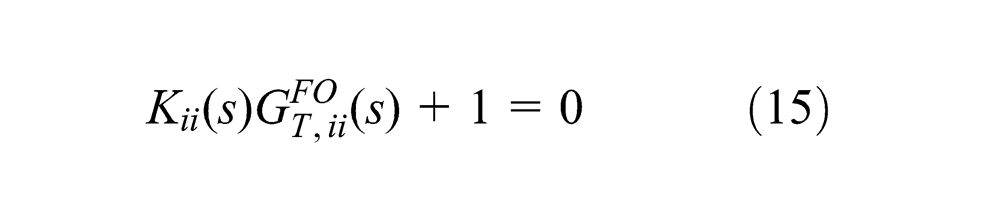
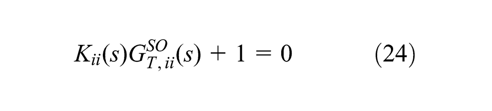
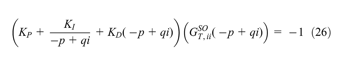
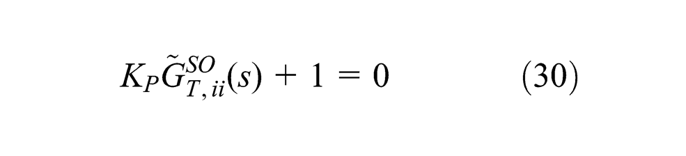
The closed-loop characteristic equation for conventional unity feedback configuration is
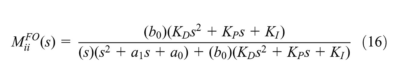
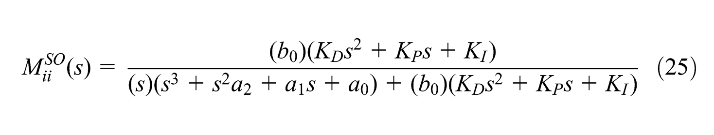
Hence, the closed-loop transfer function is
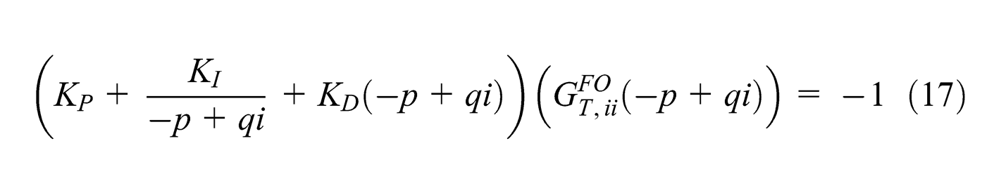
Desired time or frequency domain performance specifications can be converted into a pair of conjugate poles, for example (Åström and Hägglund, 1995).. To have dominance of the desired conjugate poles, it is necessary that the ratio of the real part of any of the other poles to must exceed (usually ) and there are no zeros nearby (Wang et al., 2009). In the proposed PID design method, the controller parameters are obtained such that all closed-loop poles are located to the left of dominant complex conjugate poles.
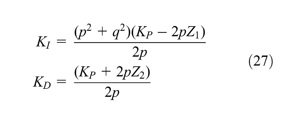
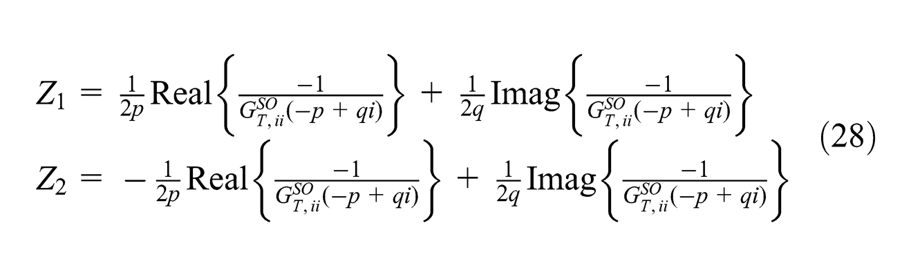
After solving and some manipulations, above equation is arranged as
where
The open-loop transfer function (s) will have one real pole at , two dominant poles at and two zeros at . The root locus is used to show the movement of the closed-loop poles for all values of a system parameter . To preserve dominance of dominant poles, a real pole must be located to the left of dominant poles . To find the value of and the remaining PID parameters, the PID design procedure is summarized as follows:
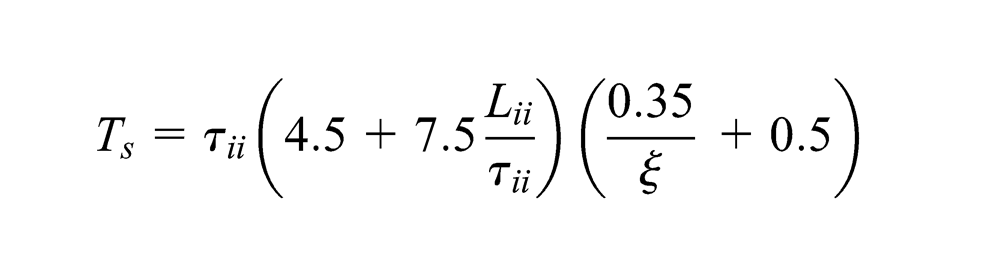
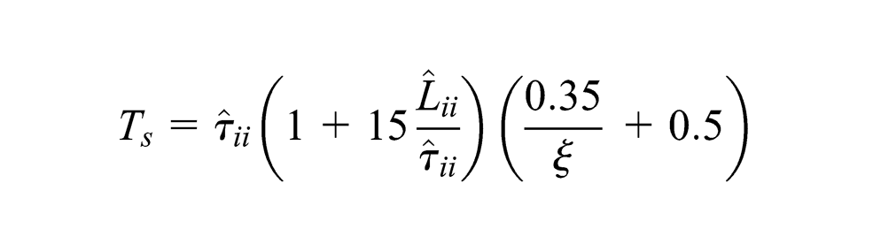
Select damping ratio . Calculate settling time and frequency (Wang et al., 2007).
Calculate dominant poles using desired characteristic equation .
Tuning of : the PID parameter for loop-1 and loop-2 is monotonically increased or decreased on-line independently and the parameters and are calculated using equation (18). The PID parameter is tuned so that the desirable performance of individual loops and the nominal system stability of the multiloop system can be conveniently achieved according to the second condition of the corollary.
To cope with the process uncertainties, tuning the adjustable parameters for each loop on-line so that robust stability is ensured according to equations (35) and (36) is suggested.
PID design method for SOPDT systems
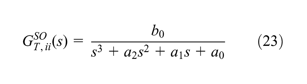
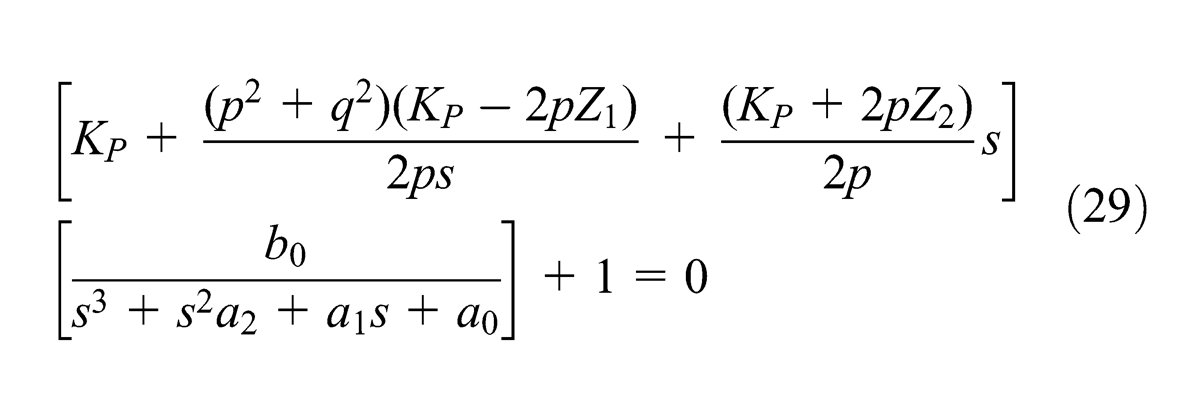
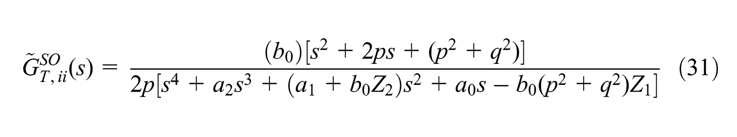
Consider a SOPDT model of the decoupled system given in equation (7). Using a first-order Taylor series approximation for the dead-time term, equation (7 can be re-written as
After solving, the above equation can be arranged as
where
The open-loop transfer function (s) will have two real poles at or two complex poles at , two dominant poles at and two zeros at . To preserve the dominance of dominant poles, the real poles at or complex poles at are located to the left of dominant poles .
Select damping ratio . Calculate settling time and frequency (Wang et al., 2007).
Calculate dominant poles using desired characteristic equation .
Tuning of : the adjustable PID parameters for loop-1 and loop-2 are tuned on-line and the parameters and are calculated according to equation (27) so that the nominal system stability and robust stability are ensured according to the second condition of the corollary and equations (35) and (36) respectively.
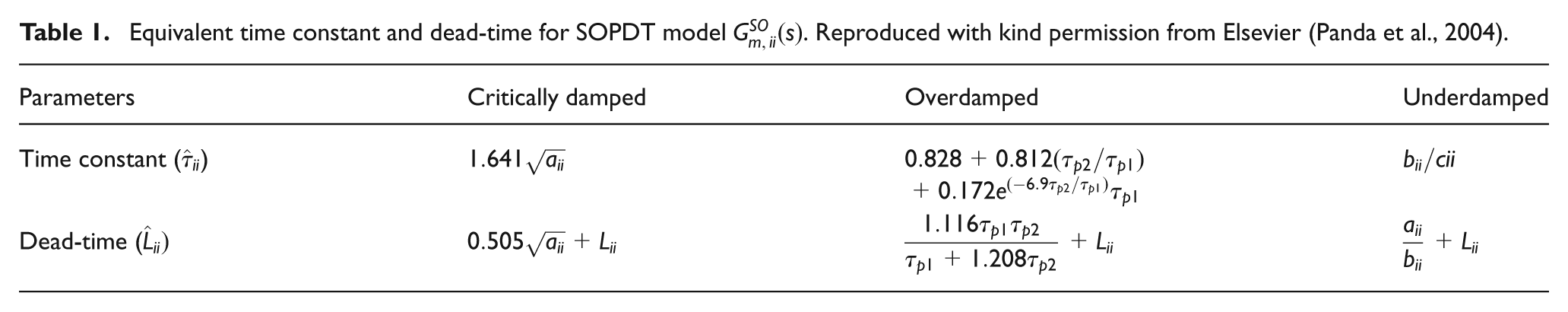
Equivalent time constant and dead-time for SOPDT model . Reproduced with kind permission from Elsevier (Panda et al., 2004).
Parameters
Critically damped
Overdamped
Underdamped
Time constant ()
Dead-time (
Stability analysis multiloop system
As higher-order decoupled subsystems are reduced to FOPDT and SOPDT models for the design of a decoupler controller matrix in section ‘Controller design method’, it is necessary to analyse the multiloop system stability so that the tuning constraints for the adjustable parameters of the proposed multiloop PID controller can be ascertained. In fact, the multiloop control structure shown in Figure 1 can be rearranged as shown in Figure 3, where is composed of the diagonal transfer functions of the process transfer function matrix ; in other words, , which connects the desired pairings between the binary system inputs and outputs. Meanwhile, is regarded as the additive uncertainty of the diagonal transfer matrix respective to FODPT/SODPT approximation.
Block diagram of a representation of a TITO control structure with additive uncertainty.
Besides, there always exist unmodelled process dynamics in practice. Hence, how to evaluate and hold the control system robust stability in presence of process uncertainty is addressed in this section, and corresponding on-line tuning of the adjustable parameters in the decoupling controller matrix is studied to cope with process uncertainties.
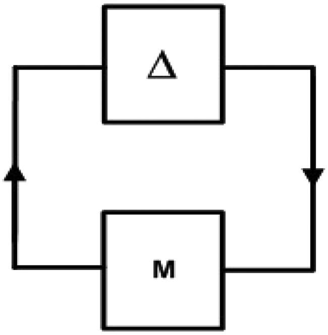
Theorem 1.Assume that the nominal system and perturbations are stable. Also consider the convex set of perturbations, , such that if is an allowed perturbation, then so is where is any real scalar such that . With this assumption, the system shown in Figure 4 is stable for all allowed perturbations if and only if any one of the following four equivalent conditions is satisfied.
Nyquist plot ofdoes not encircle the origin, , in othe words, .
.
.
.
General structure.
The corollary derived from the above theorem is utilized to identify necessary and sufficient conditions for holding the nominal system and robust stability of the TITO multiloop control structure shown in Figure 1 or equivalently, Figure 3.
Corollary 1.A TITO multiloop control system is stable if and only if
andare stable;
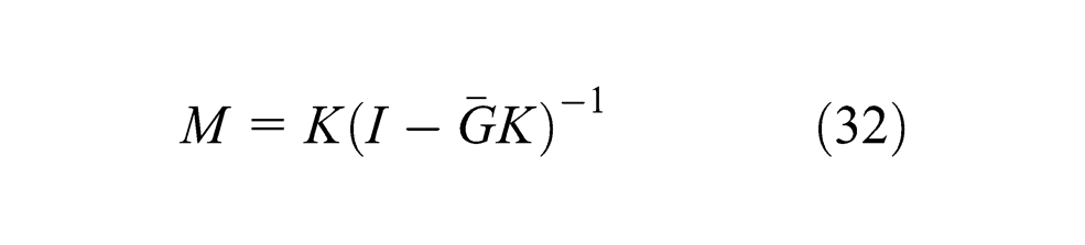
Proof of Theorem 1. Organize the equivalent multiloop control structure shown in Figure 3 in the form of the standard structure shown in Figure 4 for nominal stability analysis. Thus, the transfer matrix from the output to the input of the additive uncertainty derived is
which appears to be a diagonal transfer matrix, because and , and it is composed of two transfer functions as given in the first condition of the corollary. Hence to propose a multiloop controller in PID form, the first condition of the corollary can be intuitively identified for a stable process transfer matrix , which guarantees that the assumption of the earlier stated theorem is satisfied. Also, by substituting the additive uncertainty and equation (32) into condition 3 of the earlier theorem, the second condition is obtained directly.
It should be noted that the second condition of the corollary can be identified by examining whether the magnitude plot of the spectral radius with falls below the unity. In this manner, the acceptable tuning range of the adjustable parameters, , for loop-1 and loop-2 can be ascertained using the second condition of the corollary. In addition, for both the proposed multiloop PID controller design methods, once the design specifications, that is, dominant poles, are fixed, the relations for integral gain and derivative gain are obtained in the form of tuning parameter . Therefore, the PID controller with tuning parameter decides the location of non-dominant poles ensuring the nominal stability of the multiloop control system. This is demonstrated in the following simulation, Example 1 of section ‘Simulation study’.
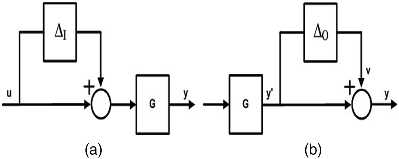
Note that in the presence of the process uncertainty, the higher-order decoupled matrix in equation (4) become very complex, and the closed-loop system tends to the stability in an intangible manner. It is difficult to address and ascertain all the stabilizing set of the multiloop controller matrix for various process uncertainties. Hence it remains as topic of research for the process control community (Skogestad and Postlethwaite, 1996; Zhou et al., 1973). A practical way to analyse the closed-loop system robust stability in the presence of commonly encountered process uncertainties such as the perturbation of process parameters, actuator output uncertainties and system output sensor measurement uncertainties, is to lump multiple sources of uncertainty into a multiplicative form (Skogestad and Postlethwaite, 1996). Here the robust stability analysis is focused on the process multiplicative input and output uncertainties, both of which are shown in Figure 5.
(a) Multiplicative input uncertainty and (b) multiplicative output uncertainty.
The process multiplicative input uncertainty, as shown in Figure 5(a), describes the actual process family , where is assumed to be stable. The process multiplicative output uncertainty, which is shown in Figure 5(b), describes the actual process family , where is also assumed to be stable. It should be noted that many other types of process unstructured or structured uncertainties may be incorporated into the types of process uncertainties mentioned above, in practice (Ogunnaike and Ray, 1979). Hence, the robust stability analysis presented in the following can be applied to a wide variety of process uncertainties.
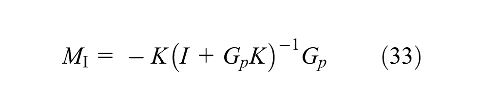
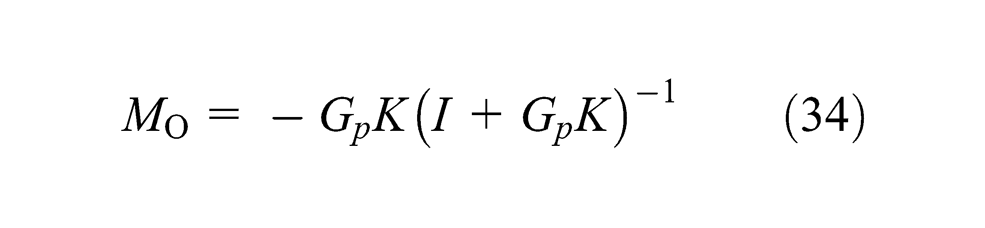
By reorganizing the perturbed control system in the form of the standard structure as shown in Figure 4 (Zhou et al., 1973) for robust stability analysis, the transfer matrix from the outputs to the inputs of and can be derived respectively as
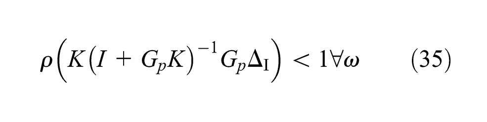
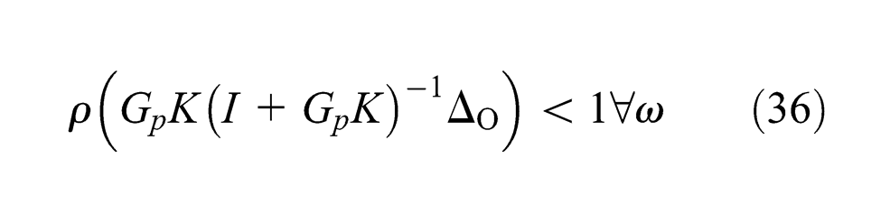
As the nominal system stability has been guaranteed by tuning the adjustable parameters , the closed-loop transfer matrix holds the stability, that is to say, is stable. Hence, and given in equations (33) and (34) are maintained stable for a stable process transfer function matrix. Therefore the aforementioned theorem is utilized to derive multiloop system robust stability conditions for tuning the adjustable parameters . Using the equations (33) and (34) with condition 3 of the aforementioned theorem gives
and
respectively. Hence, for a specified bound of or , equations (35) and (36) may be employed to evaluate the control system robust stability. Correspondingly, the spectral radius constraints given in equations (35) and (36) can be checked graphically by observing whether magnitude plots of the left sides of equations (35) and (36) with fall below the unity. In this way, the admissible range of the adjustable parameters of the decoupling controller matrix can be numerically ascertained. In fact, this robust stability check can be performed using control software packages such as the MATLAB robust toolbox (Richard and Michael, 1998).
In general, tuning each of the adjustable parameters for loop-1 and loop-2 around the steady-state gain of the process diagonal transfer functions in the first place, respectively, is recommended. Then by monotonically increasing or decreasing either of them on-line independently, the desirable output response of individual loops can be conveniently obtained. To cope with process uncertainties, namely process unmodelled dynamics, it is recommended to monotonically increase the adjustable parameters on-line so better robust stability obtained. Furthermore, if upon doing so the control system performance and robust stability still are not acceptable, a more precise process model needs to be obtained to derive the multiloop controller matrix , so as to achieve better nominal system performance and robust stability.
Simulation study
In this section, three simulation examples are included to demonstrate the performance of the proposed methods in comparison to the approximate pole placement method proposed by Wang et al. (2007, 2008), and Liu et al.’s method (Liu et al., 2005). To ensure a fair comparison, the performance (, Integral Absolute Error (IAE)) and robustness (Gain Margin (GM), Phase Margin (PM)) for the decentralized control system are calculated.
Example 1 (Vinante and Luyben column)
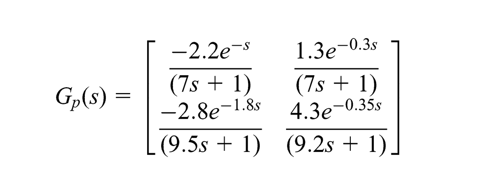
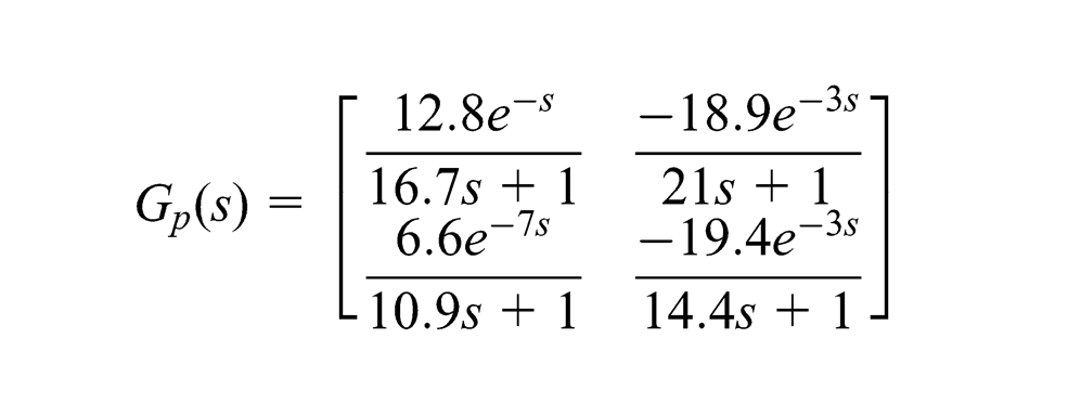
A 24-tray distillation column separating a mixture of methanol and water (Luyben and Jutan, 1986). The plant has following transfer function matrix:
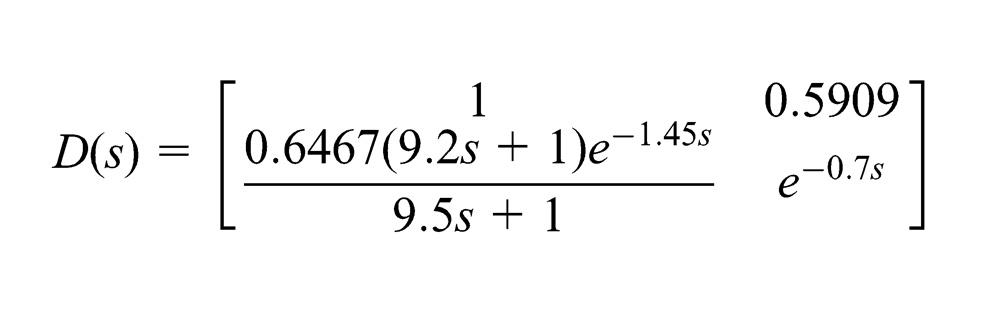
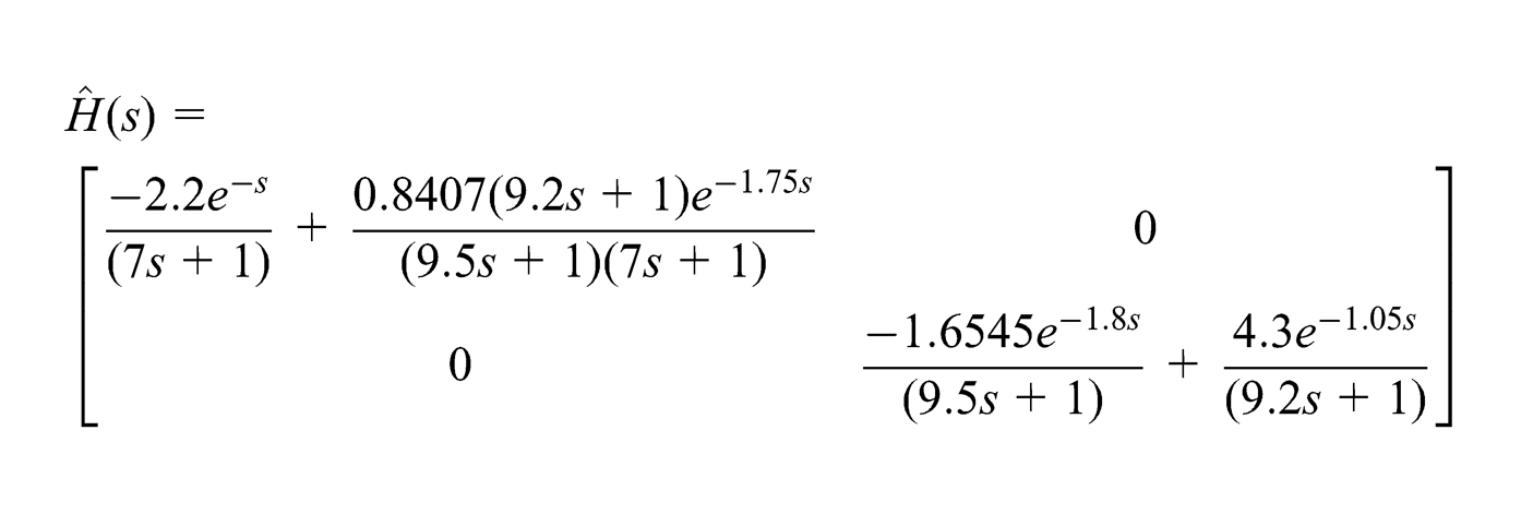
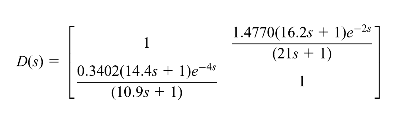
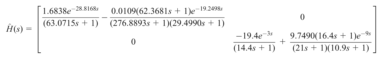
According to equation (4), the resulting diagonal system obtained is
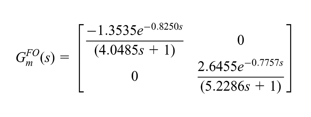
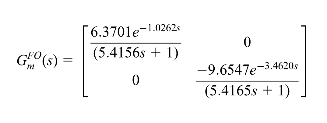
A FOPDT model of diagonal system is obtained using equation (6) as follows:
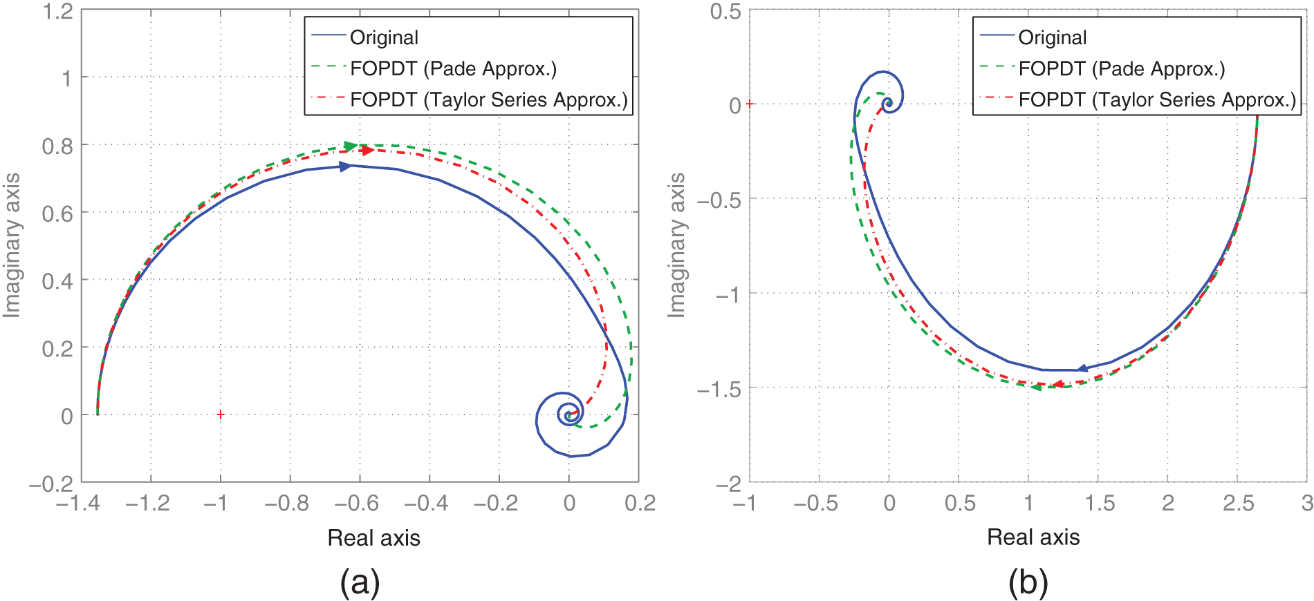
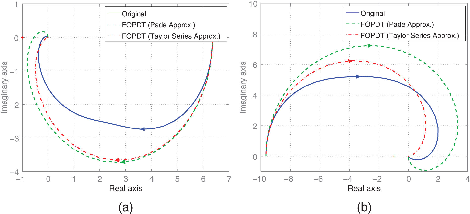
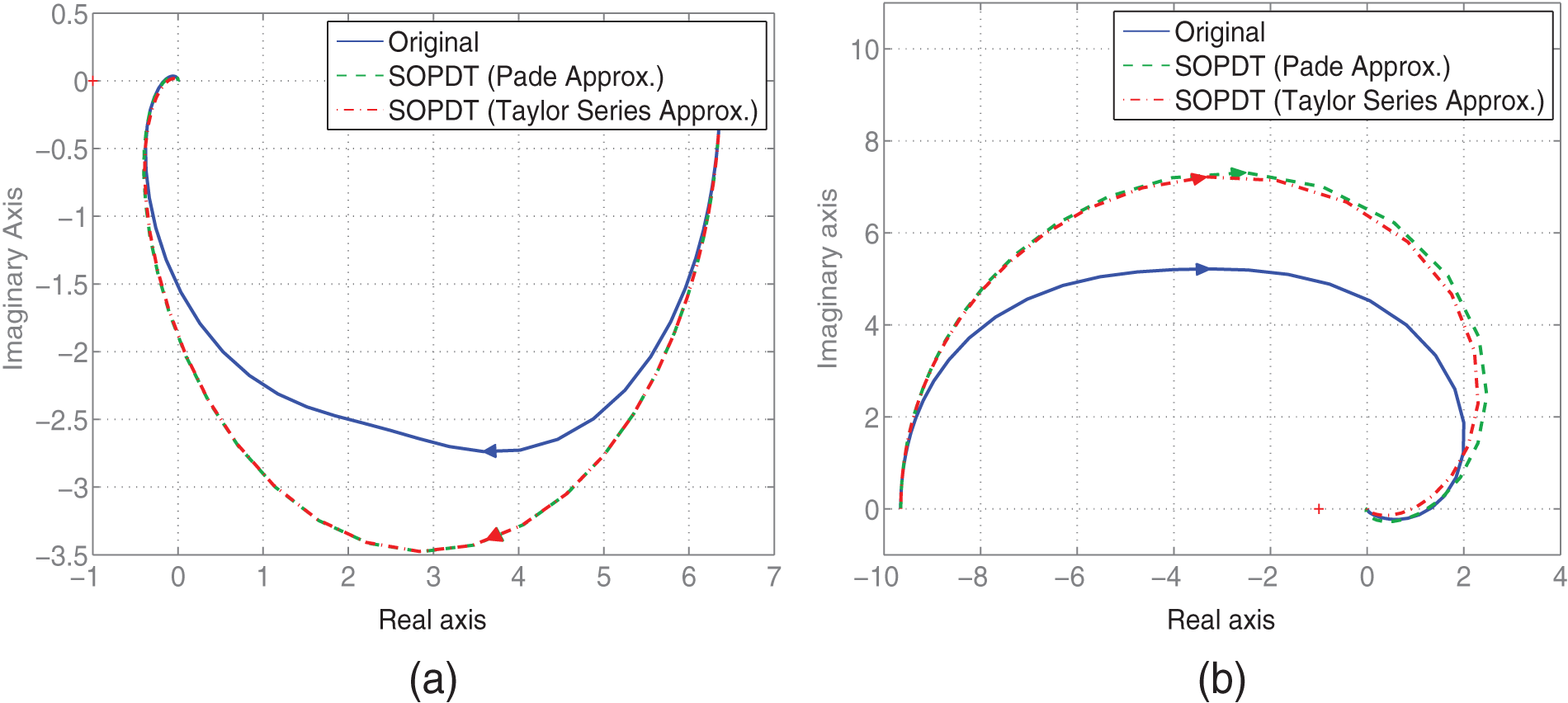
To evaluate how closely the reduced FOPDT model approximates the decoupled higher-order system, Nyquist plots are drawn. Figure 6 shows the Nyquist plots of , their FOPDT model with Pade approximation and Taylor series approximation .
Nyquist plots of , and (Example 1).
For , suppose the desired damping ratio is selected. The corresponding settling time calculated using step 1 is s. The corresponding dominant poles are . For , suppose the desired damping ratio and settling time s are selected. The dominant poles are at .
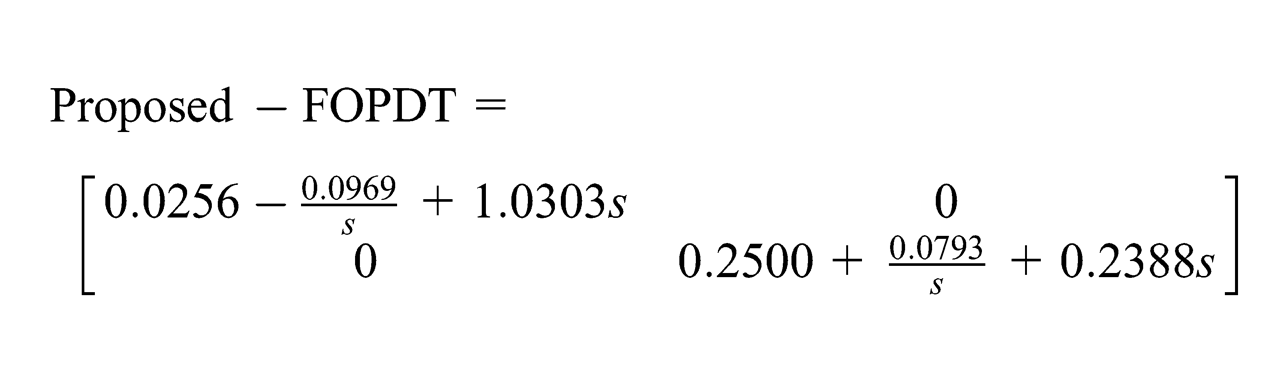
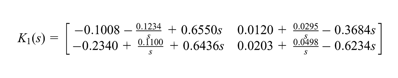
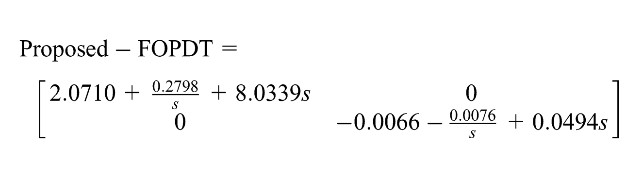
The decentralized PID controller () by the proposed method is
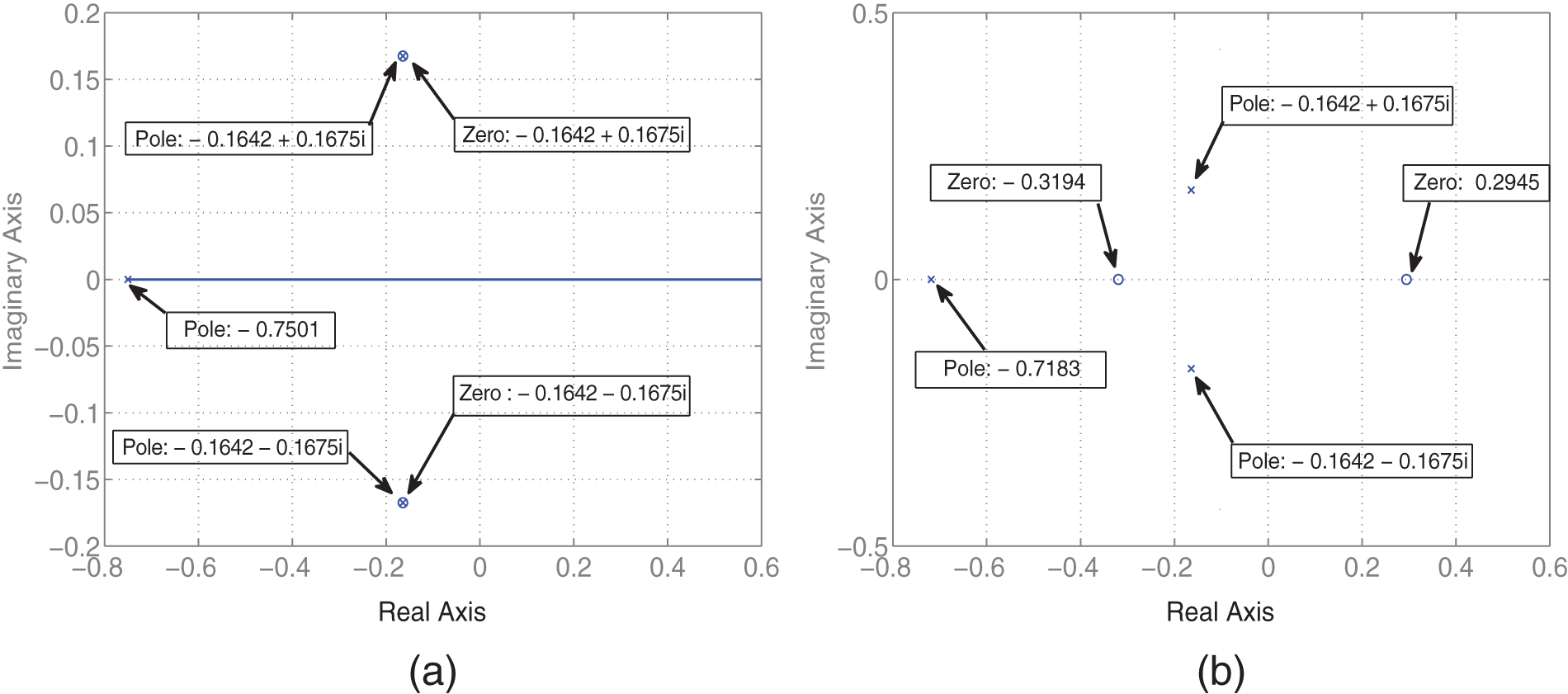
The root locus of and pole–zero plot of are shown in Figures 7 and 8.
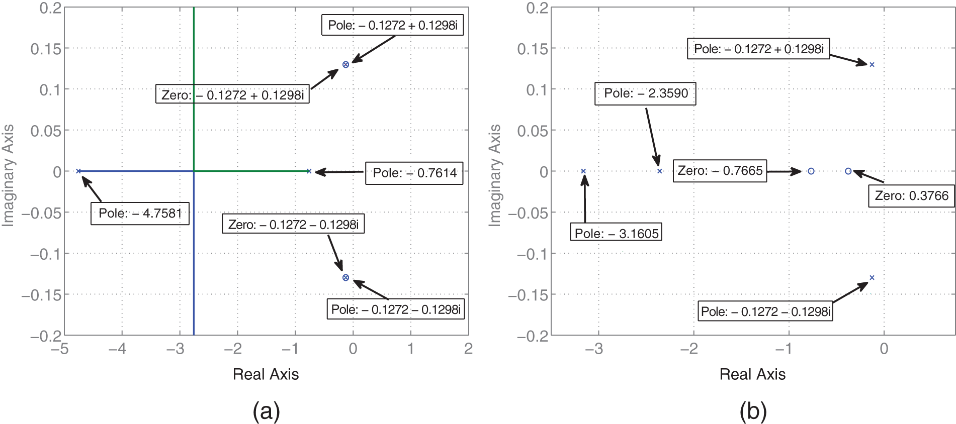
(a) Root locus of , (b) pole–zero plot of (Example 1).
(a) Root locus of , (b) pole–zero plot of (Example 1).
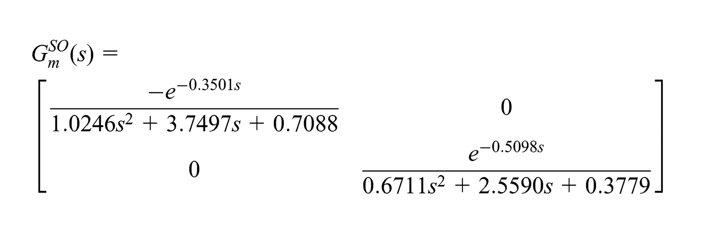
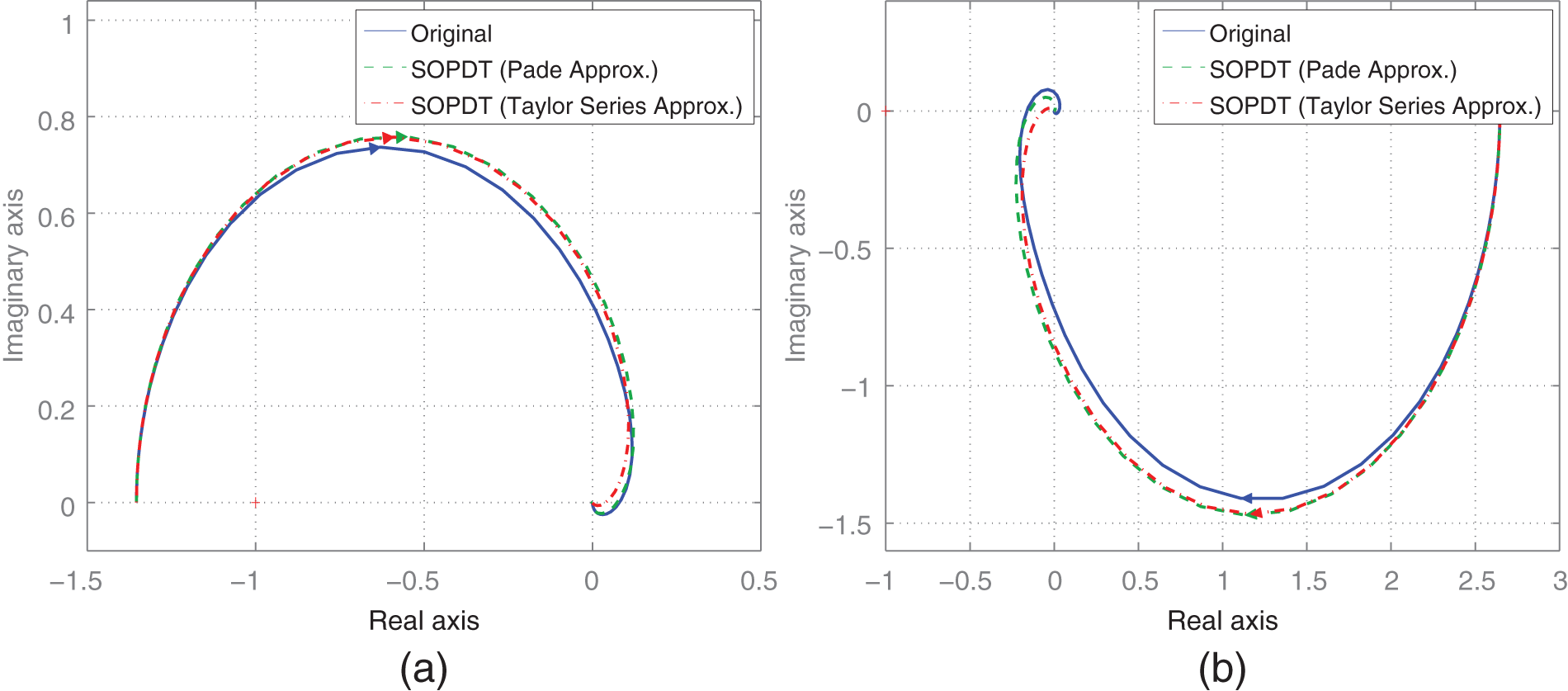
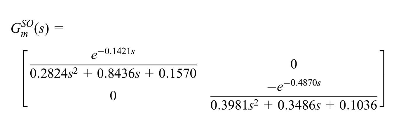
Figure 9 shows the Nyquist plots of , their SOPDT model with Pade approximation and Taylor series approximation .
Nyquist plots of , and (Example 1).
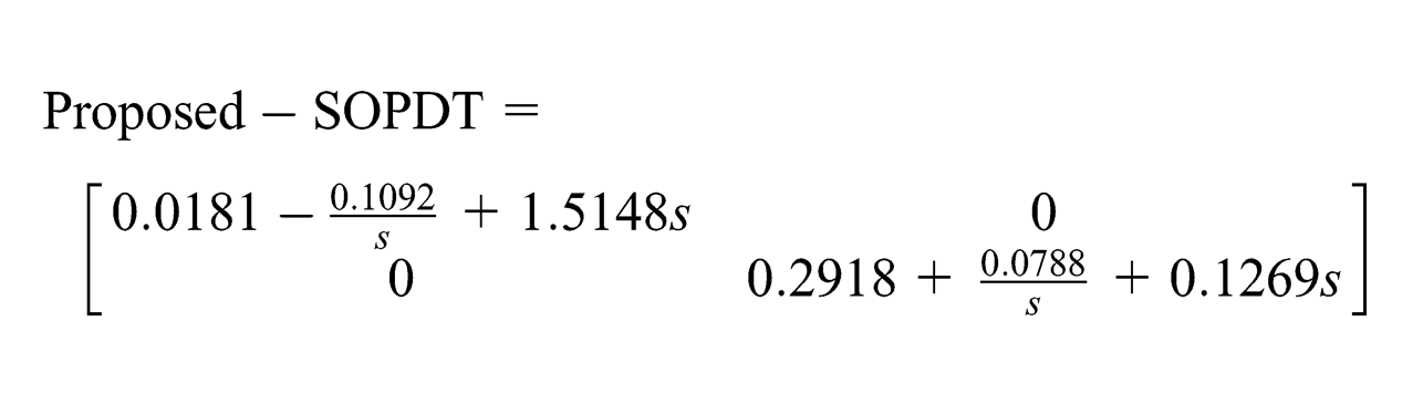
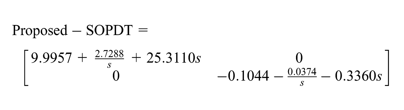
For , suppose the desired damping ratio is selected. The settling time calculated using step 1 is s. The corresponding dominant poles are at . The damping ratio is selected and settling time s is calculated for . The corresponding dominant poles are .
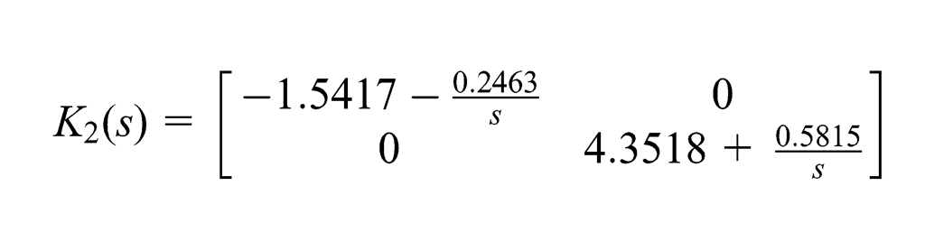
The PID controller (Proposed-SOPDT) obtained is
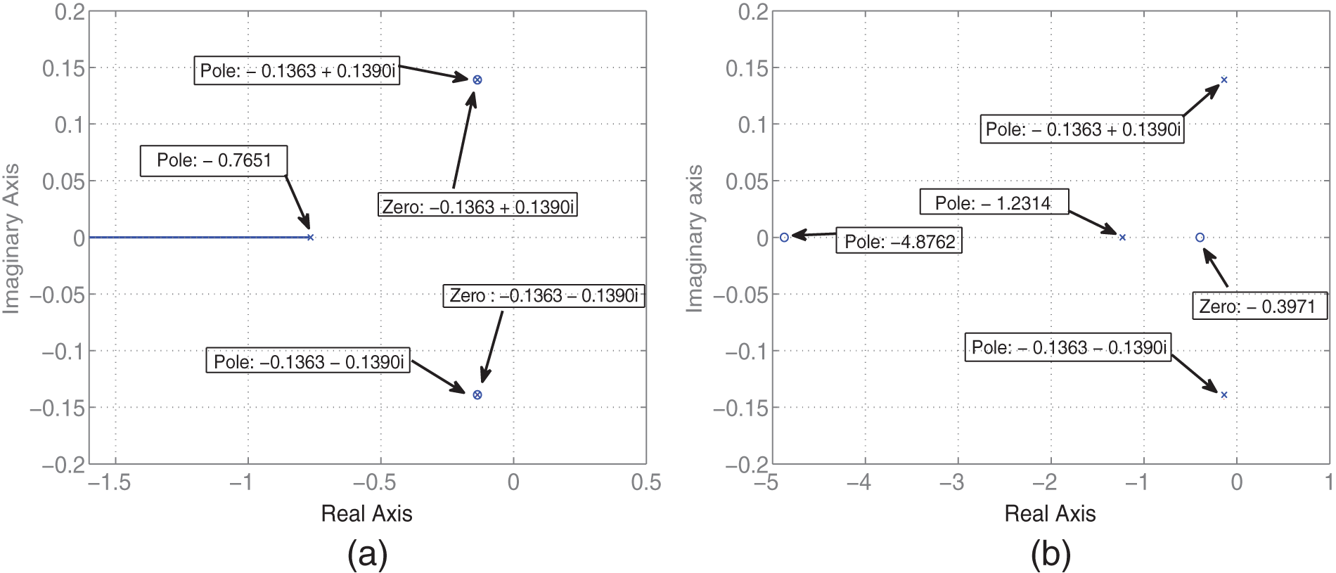
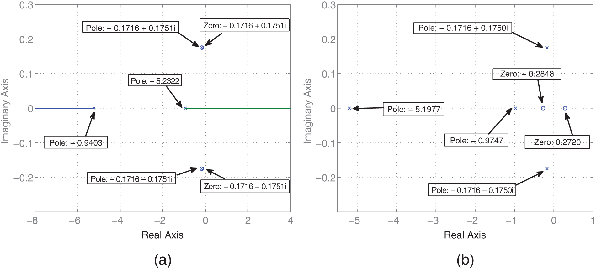
The root locus of and pole–zero plot of are shown in Figures 10 and 11.
(a) Root locus of , (b) pole–zero plot of (Example 1).
(a) Root locus of , (b) pole–zero plot of (Example 1).
Correspondingly, the magnitude plots of spectral radius used for identifying the nominal stability by both the Proposed-FOPDT and Proposed-SOPDT proposed controllers are shown in Figure 12 with solid lines.
Magnitude plots of spectral radius (Example 1).
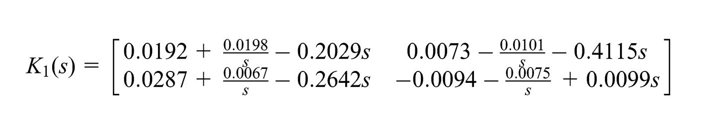
The proposed controllers are compared with Wang et al.’s multivariable controller (Wang et al., 2001, 2007, 2008) and Liu et al.’s controller (Liu et al., 2005). Wang et al.’s controller is
and Liu et al.’s controller is
To demonstrate the robust stability of the proposed control system, assume that the process multiplicative input uncertainty actually exists. This can be loosely interpreted, as binary process input actuators have up to uncertainty at high frequencies and almost uncertainty in the low-frequency range. In another case, assume that the process multiplicative output uncertainty actually exists, which can be practically viewed as that the binary process output measurements provided by the corresponding output sensors decrease by up to uncertainty at high frequencies and by almost uncertainty in the low-frequency range. The corresponding magnitude plots of spectral radius in terms of assumed (dashed line) and (dash-dot line) are shown Figure 12, and both demonstrate that the proposed control system could preserve robust stability well.
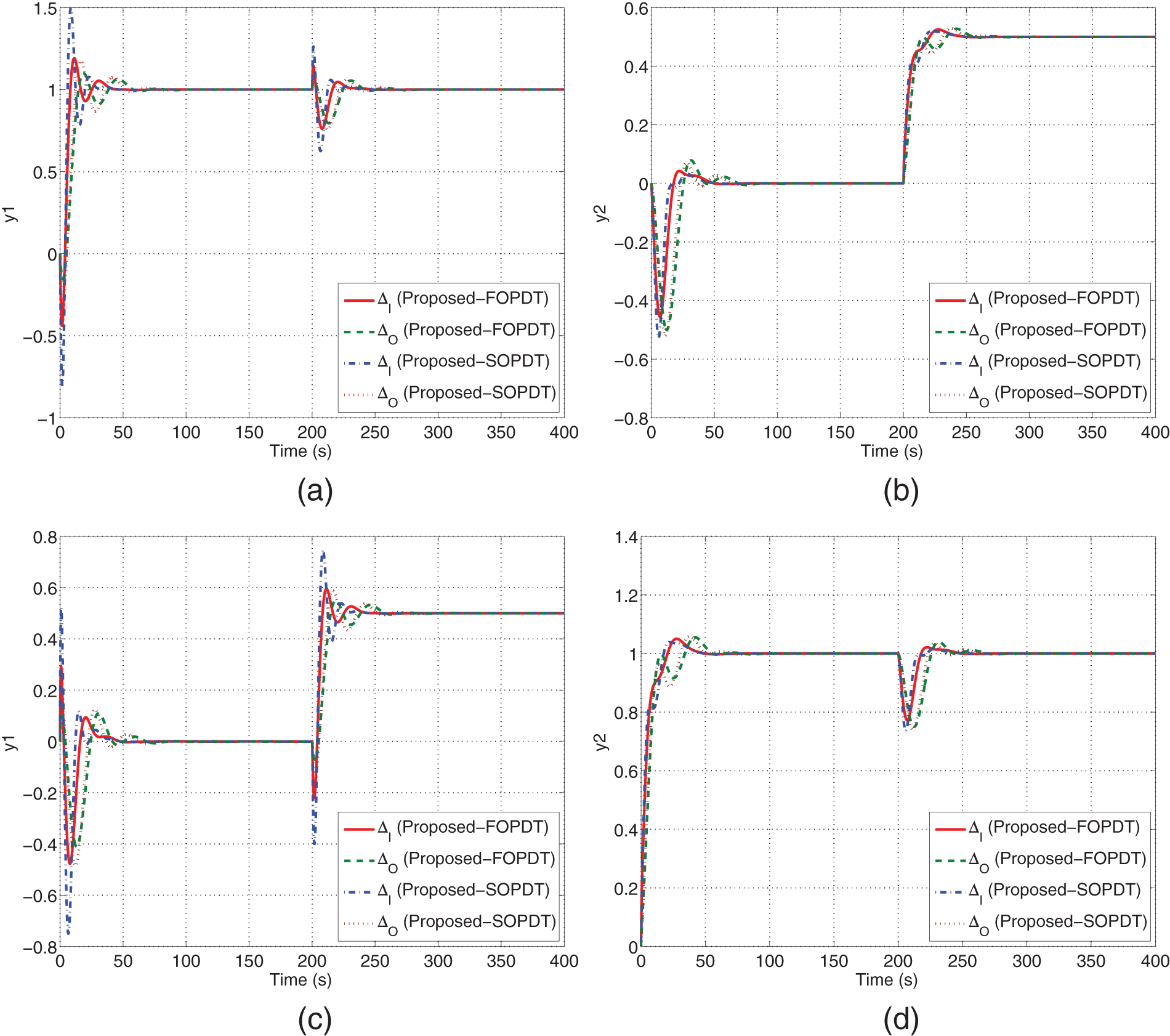
Accordingly the perturbed responses are shown in Figure 13.
Perturbed system responses (Example 1).
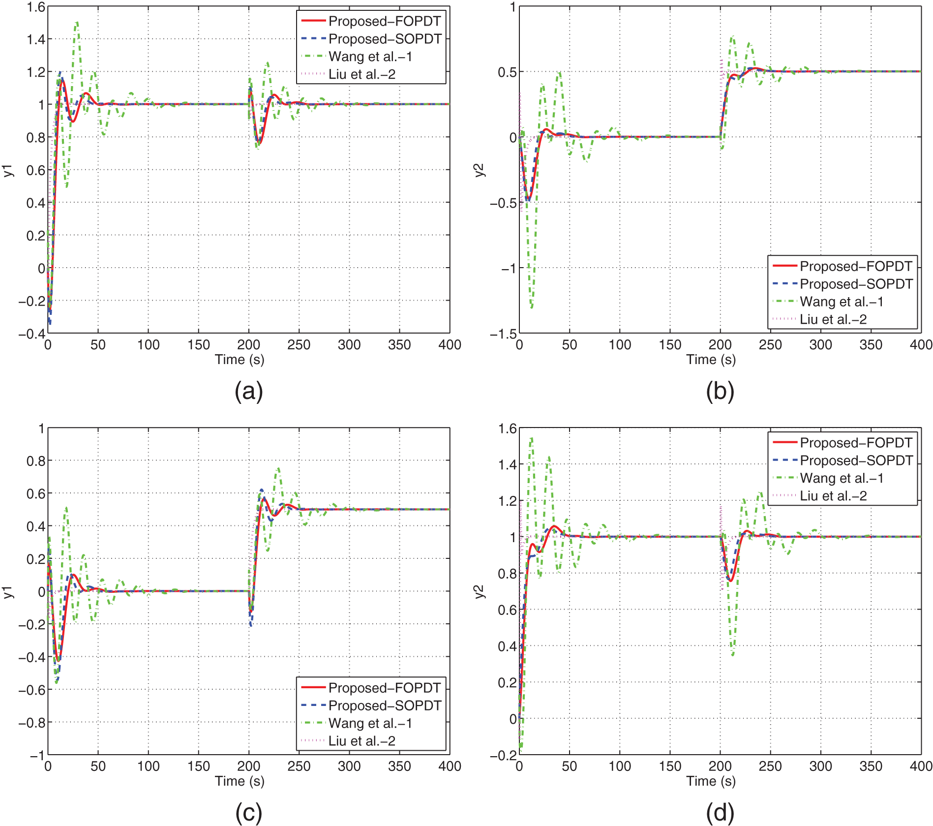
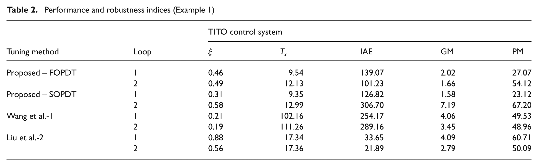
The closed-loop responses by the proposed methods, Wang et al.’s method and Liu et al.’s method are shown in Figure 14. Unit step set-point changes were sequentially introduced at s with a set-point disturbance of in other input at s. Figure 14 shows the proposed controllers provide a good performance with fast and well balanced responses in comparison to Wang et al.’s method. The performance and robustness indices are tabulated in Table 2.
Closed-loop responses to the sequential unit set-point changes (Example 1).
Performance and robustness indices (Example 1)
TITO control system
Tuning method
Loop
IAE
GM
PM
Proposed – FOPDT
1
0.46
9.54
139.07
2.02
27.07
2
0.49
12.13
101.23
1.66
54.12
Proposed – SOPDT
1
0.31
9.35
126.82
1.58
23.12
2
0.58
12.99
306.70
7.19
67.20
Wang et al.-1
1
0.21
102.16
254.17
4.06
49.53
2
0.19
111.26
289.16
3.45
48.96
Liu et al.-2
1
0.88
17.34
33.65
4.09
60.71
2
0.56
17.36
21.89
2.79
50.09
Example 2 (Wood and Berry distillation column)
Wood and Berry studied a binary distillation column, which consists of an eight-tray plus boiler separating methanol and water (Wood and Berry, 1973). The transfer function matrix is
Figure 15 shows the Nyquist plots of , their FOPDT models with Pade approximation and Taylor series approximation .
Nyquist plots of , and (Example 2).
For , suppose the desired damping ratio and settling time s are selected. The corresponding dominant poles are . For , suppose that the desired damping ratio and settling time s are considered. The desired dominant poles are . The proposed method gives the PID controller as
Figure 16 shows the Nyquist plots of , and their SOPDT models with Pade approximation and Taylors series approximation .
Nyquist plots of , and (Example 2).
For , suppose the desired damping ratio and settling time s are selected. The dominant poles are at . For , suppose the desired damping ratio and settling time s are selected. The dominant poles are .
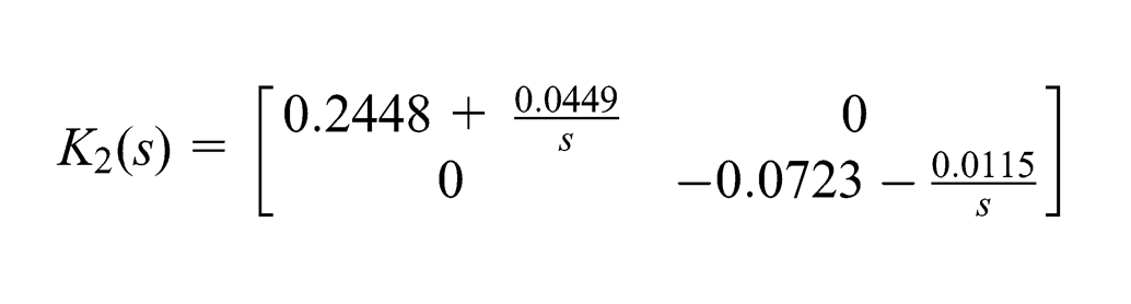
The proposed design method gives the PID controller as
The multivariable controller given by Wang et al.’s method and the controller given by Liu et al.’s method are as follows:
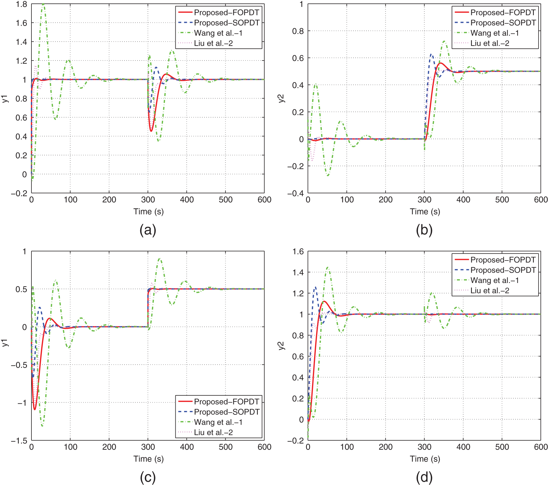
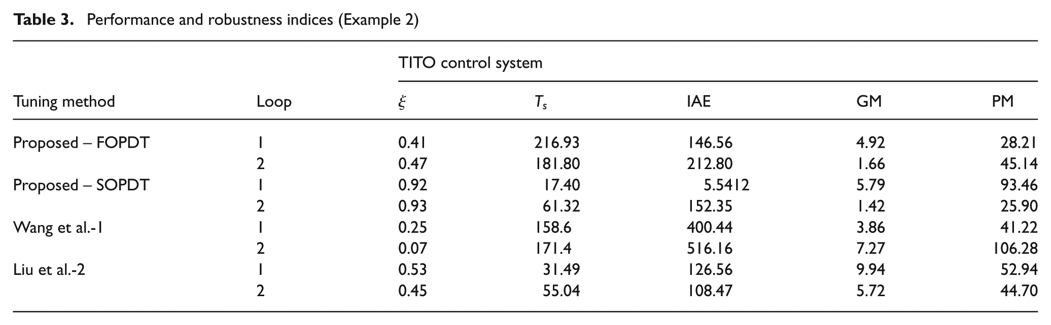
Figure 17 shows the closed-loop responses by the proposed methods, Liu et al.’s method and Wang et al.’s method, where the unit step changes in the set-point were sequentially made at s with a set-point disturbance of in other input at s. The performance and robustness indices are given in Table 3. Good performance of the proposed controllers is apparent. As shown in Table 3, the proposed methods provide good robust performance.
Closed-loop responses to the sequential unit set-point changes (Example 2).
Performance and robustness indices (Example 2)
TITO control system
Tuning method
Loop
IAE
GM
PM
Proposed – FOPDT
1
0.41
216.93
146.56
4.92
28.21
2
0.47
181.80
212.80
1.66
45.14
Proposed – SOPDT
1
0.92
17.40
5.5412
5.79
93.46
2
0.93
61.32
152.35
1.42
25.90
Wang et al.-1
1
0.25
158.6
400.44
3.86
41.22
2
0.07
171.4
516.16
7.27
106.28
Liu et al.-2
1
0.53
31.49
126.56
9.94
52.94
2
0.45
55.04
108.47
5.72
44.70
Conclusion
In this paper, two methods for decentralized PID controller design have been presented for TITO systems. The methods are based on user-defined damping ratio and settling time to achieve the desired closed-loop performance of multivariable systems. The first method is based on FOPDT models resulting from higher-order decoupled subsystems, in which the controller parameters are obtained using movement of a real pole on a real axis. In the second method, the higher-order decoupled subsystems are reduced to SOPDT models and the parameters of a decentralized PID controller are obtained by observing the movement of real or complex poles. The proposed decentralized PID design methods ensure nominal system stability and robust stability. The interaction resulting from the proposed methods is minimal and improved performance is obtained. Simulation examples demonstrate the performance of the proposed methods.
Footnotes
Funding
This research received no specific grant from any funding agency in the public, commercial, or not-for-profit sectors.
References
1.
ÅströmKJHägglundT (1988) Automatic Tuning of PID Controllers. 2nd edn.Research Triangle Park, NC: Instrument Society of America.
2.
ÅströmKJHägglundT (1995) PID Controllers: Theory Design and Tuning. 2nd edn.Research Triangle Park, NC: Instrument Society of America.
3.
ÅströmKJJohanssonKHWangQG (2002) Design of decoupled PI controllers for two-by-two system. IEE Proceedings: Control Theory and Applications149: 74–81.
4.
BaoJForbesJFMcLellanPJ (1999) Robust multiloop PID controller design: A successive semidefinite programming approach. Industrial and Engineering Chemistry Research38(9): 3407–3419.
5.
CamachoOSmithCA (2000) Sliding mode control: An approach to regulate nonlinear chemical processes. ISA Transactions39(2): 205–218.
6.
CamachoORojasRGarciaW (1999) Variable structure control applied to chemical processes with inverse response. ISA Transactions38(1): 55–72.
7.
CampoPJMorariM (1994) Achievable closed-loop properties of systems under decentralized control: Conditions involving the steady-state gain. IEEE Transaction on Automatic Control39(5): 932–943.
8.
ChenDSeborgDE (2003) Design of decentralized PI control systems based on Nyquist stability analysis. Journal of Process Control13(1): 27–39.
9.
ChienILHuangHPYangJC (1999) A simple multiloop tuning method for PID controllers with no proportional kick. Industrial and Engineering Chemistry Research38(4): 1456–1468.
10.
DoughertyDCooperD (2003) A practical multiple model adaptive strategy for single-loop MPC. Control Engineering Practice11(4): 141–159.
11.
GoodwinCGGraebeSFSalgadoME (2001) Control System Design. Upper Saddle River, NJ: Prentice-Hall.
12.
GundesANMeteANPalazogluA (2009) Reliable decentralized PID controller synthesis for two-channel MIMO processes. Automatica45(2): 353–363.
13.
HaleviYPalmorZJEfratiT (1997) Automatic tuning of decentralized PID controllers for MIMO processes. Journal of Process Control7(2): 119–128.
14.
HovdMSkogestadS (1993) Improved independent design of robust decentralized controllers. Journal of Process Control3(1): 43–51.
15.
HovdMSkogestadS (1994) Sequential design of decentralized controllers. Automatica30(10): 1601–1607.
16.
HuangHPLinFY (2006) Decoupling multivariable control with two degrees of freedom. Industrial and Engineering Chemistry Research45(9): 3161–3173.
17.
JevtovićBTMataušekMR (2010) PID controller design of TITO system based on ideal decoupler. Journal of Process Control20(7): 869–876.
18.
KhandekarAAMalwatkarGMPaterBM (2013) Discrete sliding mode control for robust tracking of higher order delay time systems with experimental application. ISA Transactions52(1): 36–44.
19.
KozákováAVeselýVOsuskýJ (2009) Decentralized controllers design for performance: Equivalent subsystems method. In: European control conference, Budapest, Hungary, pp. 2295–2300.
20.
KozákováAVeselýVOsuskýJ (2011) Direct design of robust decentralized controllers. In:Proceedings of the 18th IFAC world congress, Milano, Italy.
21.
LeeDYLeeMLeeY. (2003) MP criterion based multiloop PID controllers tuning for desired closed loop responses. Korean Journal of Chemical Engineering20(1): 8–13.
22.
LeeJChoWEdgarTF (1998) Multi-loop PI controller tuning for interacting multivariable processes. Computers and Chemical Engineering22(11): 1711–1723.
23.
LeeJKimDHEdgarTF (2005) Static decouplers for control of multivariable processes. American Institute for Chemical Engineers51(10): 2712–2720.
24.
LengareMJChileRHWaghmareLM (2012) Design of decentralized controllers for MIMO processes. Computers and Electrical Engineering38(1): 140–147.
25.
LiuTZhangWGuD (2005) Analytical multiloop PI/PID controller design for two-by-two processes with time delays. Industrial and Engineering Chemistry Research44(6): 1832–1841.
26.
LiuTZhangWGuD (2006) Analytical design of decoupling internal model control (IMC) scheme for two-input-two-output (TITO) processes with time delays. Industrial and Engineering Chemistry Research45(9): 3149–3160.
27.
LohAPHangCCQuekCK. (1993) Auto-tuning of multi-loop proportional-integral controllers using relay feedback. Industrial and Engineering Chemistry Research32(6): 1102–1107.
28.
LuybenWLJutanA (1986) Simple method for tuning SISO controllers in multivariable system. Industrial Engineering and Chemical Process Design Development25(3): 654–660.
29.
MaghadeDKPatreBM (2012) Decentralized PI/PID controllers based on gain and phase margin specifications for TITO processes. ISA Transactions51(4): 550–558.
30.
MalwatkarGMSonawaneSHWaghmareLM (2009) Tuning PID controllers for higher-order oscillatory systems with improved performance. ISA Transactions48(3): 347–353.
31.
MokadamHRMaghadeDKPatreBM (2013) Tuning of multivariable PI/PID controllers for TITO processes using dominant pole placement approach. International Journal of Automation and Control7(1–2): 21–41.
32.
MusmadeBBMunjeRKPatreBM (2011) Design of sliding mode controller to chemical processes for improved performance. International Journal of Control and Automation4(1): 15–31.
33.
NordfeldtPHägglundT (2006) Decoupler and PID controller design of TITO systems. Journal of Process Control16(9): 923–936.
34.
OgunnaikeBARayWH (1979) Multivariable controller design for linear systems having multiple time delays. American Institute for Chemical Engineers25(6): 1043–1056.
35.
PandaRCYuCCHuangHP (2004) PID tuning rules for SOPDT systems: Review and some new results. ISA Transactions43(2): 283–295.
36.
RichardYCMichaelGS (1998) Robust Control Toolbox User’s Guide. Natick, MA: The MathWorks Inc.
37.
ŠekaraTBMataušekMR (2010) Revisiting the Ziegler-Nichols process dynamics characterization. Journal of Process Control20(3): 360–363.
38.
ShenSHYuCC (1994) Use of relay-feedback test for automatic tuning of multivariable systems. American Institute for Chemical Engineers40(4): 627–646.
39.
ShinskeyFG (1996) Process Control Systems: Application, Design and Tuning. New York, NY: McGraw-Hill.
40.
ShiuSJHuangSH (1998) Sequential design method for multivariable decoupling and multiloop PID controllers. Industrial and Engineering Chemistry Research37: 107–119.
41.
SkogestadSMorariM (1989) Robust performance of decentralized control system by independent design. Automatica25(1): 119–125.
42.
SkogestadSPostlethwaiteI (1996) Multivariable Feedback Control: Analysis and Design. New York, NY: John Wiley & Sons.
43.
TanKKFerdousR (2003) Relay-enhanced multi-loop PI controllers. ISA Transactions42(2): 273–277.
44.
TavakoliSGriffinIFlemingPJ (2006) Tuning of decentralised PI (PID) controllers for TITO processes. Control Engineering Practice14(9): 1069–1080.
45.
VuTNLLeeM (2010) Independent design of multi-loop PI/PID controllers for interacting multivariable processes. Journal of Process Control20(8): 922–933.
46.
WangQGHangCCYangXP (2001) Single-loop controller design via IMC principles. Automatica37(12): 2041–2048.
47.
WangQGHuangBGuoX (2000) Autotuning of TITO decoupling controllers from step tests. ISA Transactions39(4): 407–418.
48.
WangQGLeeTHLinC (2003) Relay Feedback: Analysis, Identification and Control. London: Springer.
49.
WangQGLeeTHZhangY (1998) Multiloop version of the modified Ziegler-Nichols method for two input two output processes. Industrial and Engineering Chemistry Research37(12): 4725–4733.
50.
WangQGLiuMHangCC (2007) Approximate pole placement with dominance for continuous delay systems by PID controllers. The Canadian Journal of Chemical Engineering85(4): 549–557.
51.
WangQGYeZCaiWJ. (2008) PID Control for Multivariable Processes. Berlin/Heidelberg: Springer Verlag.
52.
WangQGZhangZÅströmKJ. (2009) Guaranteed dominant pole placement with PID controllers. Journal of Process Control19(2): 349–352.
53.
WoodRKBerryMW (1973) Terminal composition control of binary distillation column. Chemical Engineering Science28(9): 1707–1717.
54.
ZhouKMDoyleJCGloverK (1998) Essentials of Robust Control. Upper Saddle River, NJ: Prentice-Hall.