






Abstract
A supply chain management system is defined as communications among suppliers, plants, distribution centres, retailers and demand stimulus. These systems are large scale and multi-agent, and therefore a decentralized control method must be used. Also, demand forecasting, as a challenge in production management, can be estimated by advanced methods or modelled using demand forecasting functions. In this paper, a new decentralized receding horizon control method is used to achieve customer contentment and low-cost inventory in a complete chain of supply, manufacture, assembly, warehouse, distribution and retail units. The main novelty of the method returns to the use of both the move suppression term and the look-ahead idea to increase robustness and smoothness in a supply chain containing assembly units. Also, a Kalman filter estimator is applied to estimate states and output variables. For this purpose, a suitable model and appropriate optimal control method are developed. Finally, the efficiency is indicated regarding simulation results.
Keywords
Introduction
In the new worlds, to achieve a competitive advantage is one of key elements of success. Unlike the traditional case, which only applies a manager’s knowledge, modern supply chain management, as an advantage, uses advanced mathematical theories and tries to coordinate whole product chain. Supply chains are structured as different stages including supply units, manufacturing units, assembly units, warehouse units, distribution units, retailers and finally customers (Beamon, 1998; Igor, 2008; Perea-Lopez and Ydstie, 2003). Two types of communications can be defined among the supply chain units, which are the goods flow and the order flow. An aggregation between the stages and the flows introduces the supply chain management system. Most details of the supply chain management system are shown in the Figure 1. In this organization, the orders flow from downstream to upstream units, and the goods (materials) flow in the reverse direction.
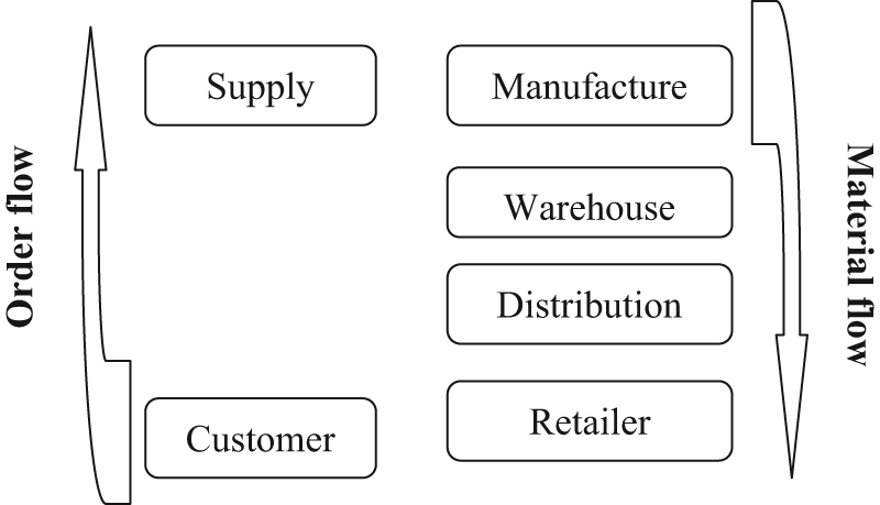
Supply chain management system.
Efficient management of a supply chain depends on appropriate identification of the flows and scheduling of material flow to reach optimal customer satisfaction. In recent decades, a variety of control methods, including classic and modern methods, direct and indirect methods, centralized and decentralized visions, have been studied to improve inventory/cost control in supply chain management systems with handling desired optimization objectives and chain performance measures (Seferlis and Giannelos, 2004).
Model predictive control (MPC), because of its abilities in efficient solving of multi-input–multi-output problems on a rolling horizon has been used in past research in the field of production/inventory management. Perea-Lopez and Ydstie (2003) applied a predictive method for scheduling of distribution systems with a simplified optimization model for manufacturing function. This optimization problem considers deterministic demands. In this case, employing robust control and even complicated inventory control is unnecessary (Kapsiotis and Tzafestas, 1992). A discrete time difference model is developed in Tzafestas and Kapsiotis (1997). The model is intuitive for use in large-scale supply chains and can track all events and flows in a network. On the other hand, an MPC approach as a damper on the bad effect of stochastic uncertainties is used.
A formal type of MPC is centralized, which optimizes all control inputs in a particular problem among a receding horizon (Scattolini, 2009). In some situations, such as large-scale applications that are often seen in power transmission systems, water distribution systems, waste water treatment, traffic control systems, production and planning systems and economic systems, a centralized method may not be operational for technical or commercial reasons (Chopra and Meindl, 2004; Sarimveis et al., 2008). In such conditions, design engineers should convert the centralized system to decentralized units to create an adaption between employing distributed control schemes and the system model. Distributed (decentralized) MPC uses past and present local control actions to predict local future inputs in each subsystem (Camacho and Bordons, 2004; Findeisen et al., 2007). Other advantages of decentralized mode are lower computational loads and lower error probability (Agachi et al., 2009; Towill, 2008).
In this paper, a multiple local receding horizon control method is applied to a complete supply chain management system, which consists of suppliers, plants, assemblers, warehouses, distributors and retailers. Receding horizon control, a version of MPC in which all parts model in state space regarding the abilities of MPC in control of large dimension, introduces a striking method for facing inventory management systems. Also, a distributed Kalman filter estimator and a look-ahead scheme are employed to gain a correct estimation of the variables’ situations and the needed horizon. The speed penalty and even the acceleration penalty, some of the efficient solutions in the robustness field, in this paper are used for robustness and softness enhancements in the calculations. Regarding the organization of this paper, the next part is a model description based on a famous difference model. Then, a decentralized receding horizon control approach with a Kalman filter and a coordination method of agents for implementation on a supply chain system is addressed. Finally, simulations and comparisons illustrate the advantages of the methods considered and the tools in the efficient management of supply chains; then, a conclusion gathers the main challenges and focuses on vital notes.
General dynamic model of supply chain management system
Supply chain management system can be described by a discrete time dynamic model, including difference equations of inventories and goods shipment quantities. The model can be extended to each type of large-scale supply chain. One type of product is manufactured at plants P, using the various supplied resources from suppliers S. With regard to Figure 1 (material flow), in the first step, raw materials are forwarded to plants and after the manufacturing process, products are sent to assembling units A. In the next phase, final products are subsequently transported to warehouses W, distribution centres D, retailers R, and final customers so that a level of safety stock should be kept. Retailers receive orders of various products from different customers with varying degrees of uncertainty.
A discrete time difference model is used to describe supply chain dynamics. Times of the model are often based on hours, days or weeks. Times or in the other words, decision times, depend on the properties of the supply chain (Seferlis and Giannelos, 2004).
In the assumed model of supply chain, suppliers S, plants P, assembly centres A, warehouses W, distribution centres D and retailers R are the nodes of the system. Upstream nodes for each node, i, are indexed by
The following equations indicate clearly storing, kipping stock and distribution management at time instances t and t+ 1 around each node, and consider the back order. The first and second equations are defined to analyse the material flow and the third equation returns to the order flow. As a result, the first equation is applied as:
where
The second equation is constructed for retailer nodes and indicates the logistic step in retailers. With regard to this equation, the inventory amount in time t in each retailer node is equal to the summation of imported goods minus the delivered items inventory in the past time instance.
The ultimate target of supply chain management is to achieve a reasonable level of customer satisfaction. However, besides this, the levels of back orders and terminated orders should be controlled. Another equation shows the situation of unsatisfied demands. These demands are defined as back orders for each product and time. In order to reach this, the following equation is introduced:
where di denotes the demand for product at retailer node i and time t; fi denotes the delivered products to customers from retailer node i and at time t ; ui denotes the amount of unfulfilled orders for the product at retailer node i and time t, because the chain failed to satisfy them in a conditional time. Unfulfilled orders, or in the other words continual back orders, are often expressed by a percentage of demands at time t.
Multi-agent constraint receding horizon control with full estimated state variables
From the viewpoint of control theory, control aims in the field of economics and management are categorized into two sets: cost and satisfaction. Cost in the supply chain is often defined as inventory saving cost or transportation cost. Also, satisfaction is dependent on on-time delivery of goods to final customers. With regard to this, the inherent measures of supply chain management performance can be summarized in improving customer satisfaction (responsibility) and spending less money (performance). Satisfaction can be earned by the minimization of back orders over the appropriate prediction horizon. The back orders have considerable harmful impact on the chain reputation and can increase the level of the accumulated demands and orders over time.
Supply chains are full of forecasts in the field of demand or structural models or even social effects of the market. On the other hand, past and present control actions affect the future control of the system. This introduction can guide the research toward a modern control method, named receding horizon control. In this method, future response is predicted over the specified time horizon with a described model such as the noted difference model noted in Equations (1)–(3). In the model, state variables are inventory levels at the storage nodes s, and the back orders b, at the order receiving nodes. The input variables are the product quantities transferred through the available channels l, and the delivered amounts to customers f. Also, all the state variables: the inventory levels s, and the back orders b can be chosen as the output variables. The inventory setpoints are time invariant parameters, but can be considered variant in special situations. The receding horizon control method has two phases; one of which is model identification and another is optimization. Equations (1)–(3) are the outcomes of the model identification. In the next stage, the control variable (input variable) is calculated by the optimization of performance index of the supply chain in which the model and system’s constraints are inserted. These phases at each time are repeated and the first control array in the calculated vector is implemented.
The performance index including a set of inventory, transportation, transportation changes and back order is presented as the following mathematical form.
The performance index C consists of two principal terms. The first is about output costs including the tracking cost and the back order cost, and is optimized over the prediction horizon p by quadratic programming method. The tracking cost, as a penalty on inventory levels, tries to close up the available inventory levels in plants, assembly centres, warehouses, distribution centres and retailers to predetermined setpoints sid, which may be time variant or time invariant. The back order cost, which penalizes back orders for retailers, tries to close up the available back order levels to zero.
The first term of the performance prediction can be used in the role of customer importance. The second term is about input costs, including the transportation cost and changes the cost of the transported product quantity from a node to other nodes throughout the supply chain, optimized over the control horizon c by the quadratic programming method. The transportation cost is used to restrain unnecessary shipping without losing customer satisfaction. Cost changes of the transported product quantity or in the other words, the transportation deviations cost, penalizes the deviations of the control variables from the corresponding quantity in the previous time. In fact, this cost is equivalent to a penalty on the rate of changes in the control variables and is called the move suppression term, which tends to decrease sudden decision and shipping. Therefore, the second term of the performance prediction can be used in the role of the functional cost optimizer because shipping of goods in large volumes and the aggressive changes of transportation can be unfeasible and costly. Besides the merit of the move suppression term, slowing the dynamic response because of use has a bad effect on the control performance and is a disadvantage.
The weights
In Equation (4), the centralized performance index optimizes throughout the supply chain system (Equations 1–3) on a set of the input and output constraints. The constraints are often based on physical constrains such as the storage and transportation capacities, but may sometimes be designed for some functional goals such as decreasing the back orders or omitting the aggressive dynamic responses.
If supply chains are modelled by Equations (1)–(3), they can be controlled by a centralized receding horizon control method as seen in Figure 2. Accordingly, a supervisor looks up to the whole supply chain and generates proper manipulator variables to achieve the best fit.
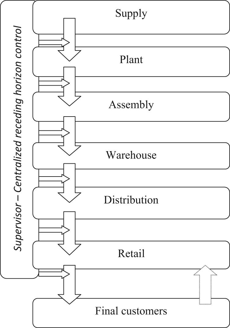
Centralized receding horizon control scheme.
As mentioned earlier, some merits of decentralized control guided researchers toward local control of systems. For this purpose, the integrated performance index, Equation (4), as a summation of manufacturing, assembling, warehousing, distributing and retailing costs (Equation 5), should be divided into five independent cost functions as follows.
The cooperation procedure of the multi-agent receding horizon control for supply chain management is illustrated in Figures 3 and 4. With regard to Figure 3, the first stage of decentralized receding horizon control after the model decentralization is optimization on the latest units, namely the retailers with Equation (10), in which customer demands are considered measurable disturbances and actuate the system. The first array of each joint control variable between the retailers and the distribution centres, as a certain measurable disturbance, is sent to the corresponding distribution node. In the next step, the local agent (the local receding horizon control) of the distribution centres receives the quantities of coupled links of the downstream nodes (retailers) as measurable disturbances and then optimizes its own policies using Equation (9), and sends recent policy to the joint links of warehouses. Similarly, in the third step, the receding horizon controller corresponding to the warehouses (Equation 8) will be optimized on local policy and then the first array of calculated decision variables will sent to the corresponding nodes in the assembly unit. In the next stage, the local agent of the assembly centres receives the joint quantities of the warehouse echelon as measurable disturbances and optimizes its own policies using Equation (7), and sends common decisions to the plants. The latest step of control in a period is employed to solve Equation (6) with the measurable disturbance of common variables from the assembly to the plant and to request the needed material for goods manufacturing.
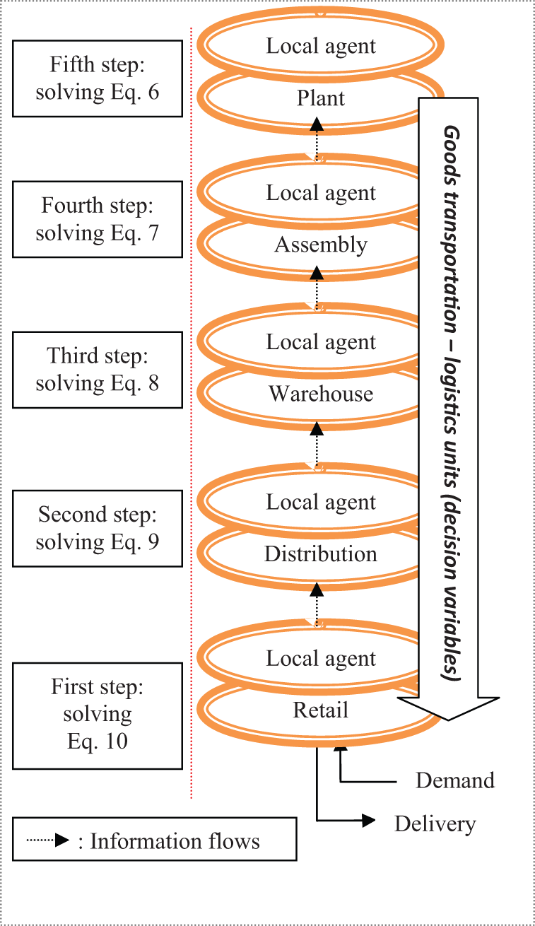
Hierarchical decentralized receding horizon control for supply chain management.
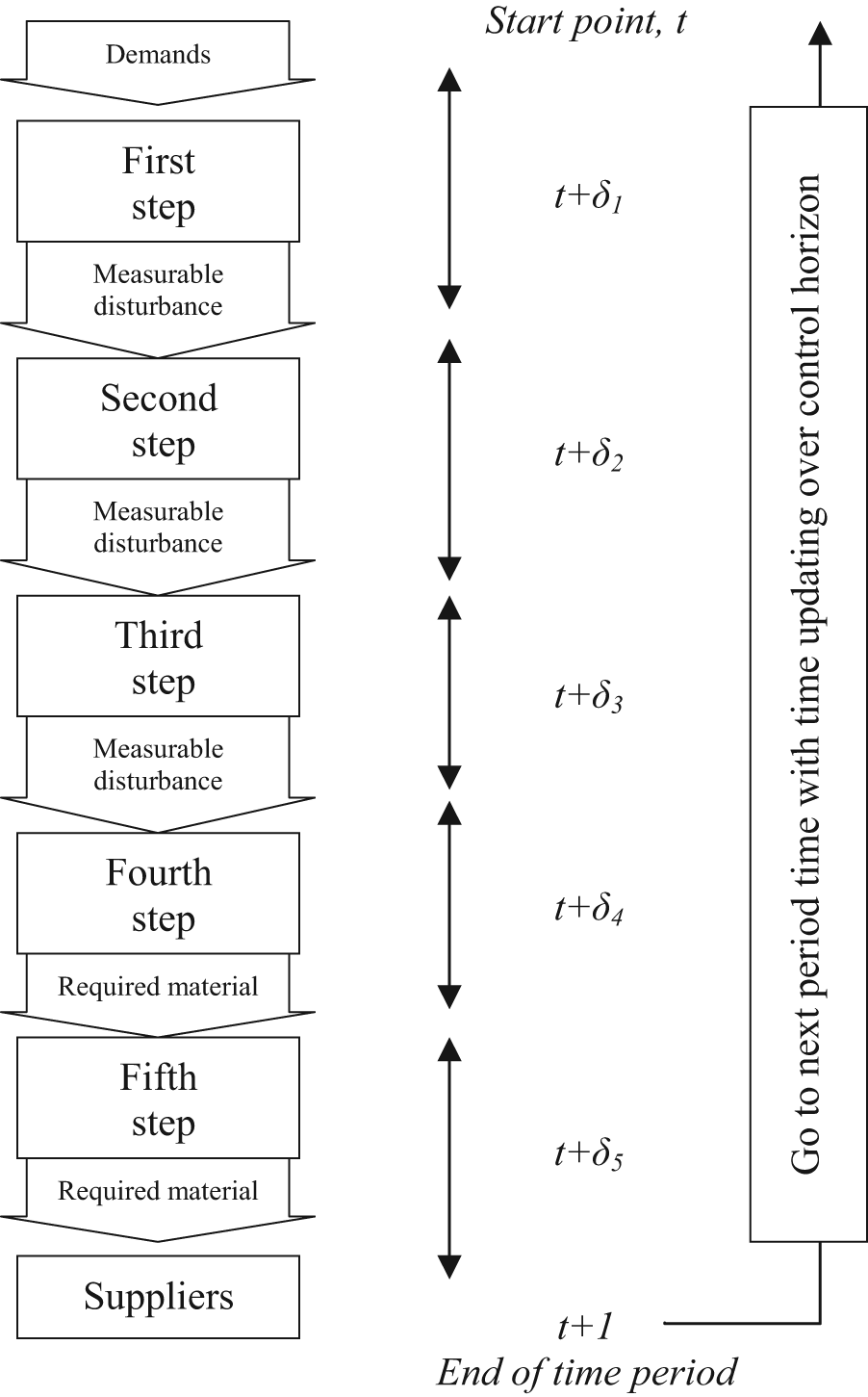
Schematic cooperation procedure of multi-agent receding horizon control for supply chain management.
With regard to Figure 4, in which time intervals are indexed as
Some state variables may be unavailable or have uncertainty, and must be estimated by an advanced estimator such as the Kalman filter. This paper employs a full Kalman estimator, in which all state variables are estimated over a certain prediction horizon; with regard to this, note that whole the system is observable. Also, in the case of the decentralized control, the decentralized Kalman filter estimates independently the local state variables for each echelon. Equations (1)–(3) are reformulated using the Kalman estimator as follows:
where KE denotes the Kalman estimator function,
Simulations
In this paper, a single-product supply chain consisting of two nodes in the supply unit, three nodes in the plant echelon, five nodes in the assembly unit, eight nodes in the warehouse echelon, 30 distribution centres and 42 retailers is considered. The quantities of inventory levels, inventory capacities, back orders, lost orders, measurable disturbances and transferred goods are considered average amounts for each specific echelon. All the nodes in the consecutive echelons are linked together, or, in the other words, there is a possibility of goods transportation between successive units. According to Table 1, the necessary data for simulation and implementation, namely inventory target levels, maximum capacities of nodes, transportation cost ratios for each supply channel, inventory weights for nodes of each echelon, back order weights for the retailer nodes, initial amounts of inventory for nodes in each echelon and transportation delays of different echelons, are given with regard to real cases in the field of supply chain management.
Supply chain data.
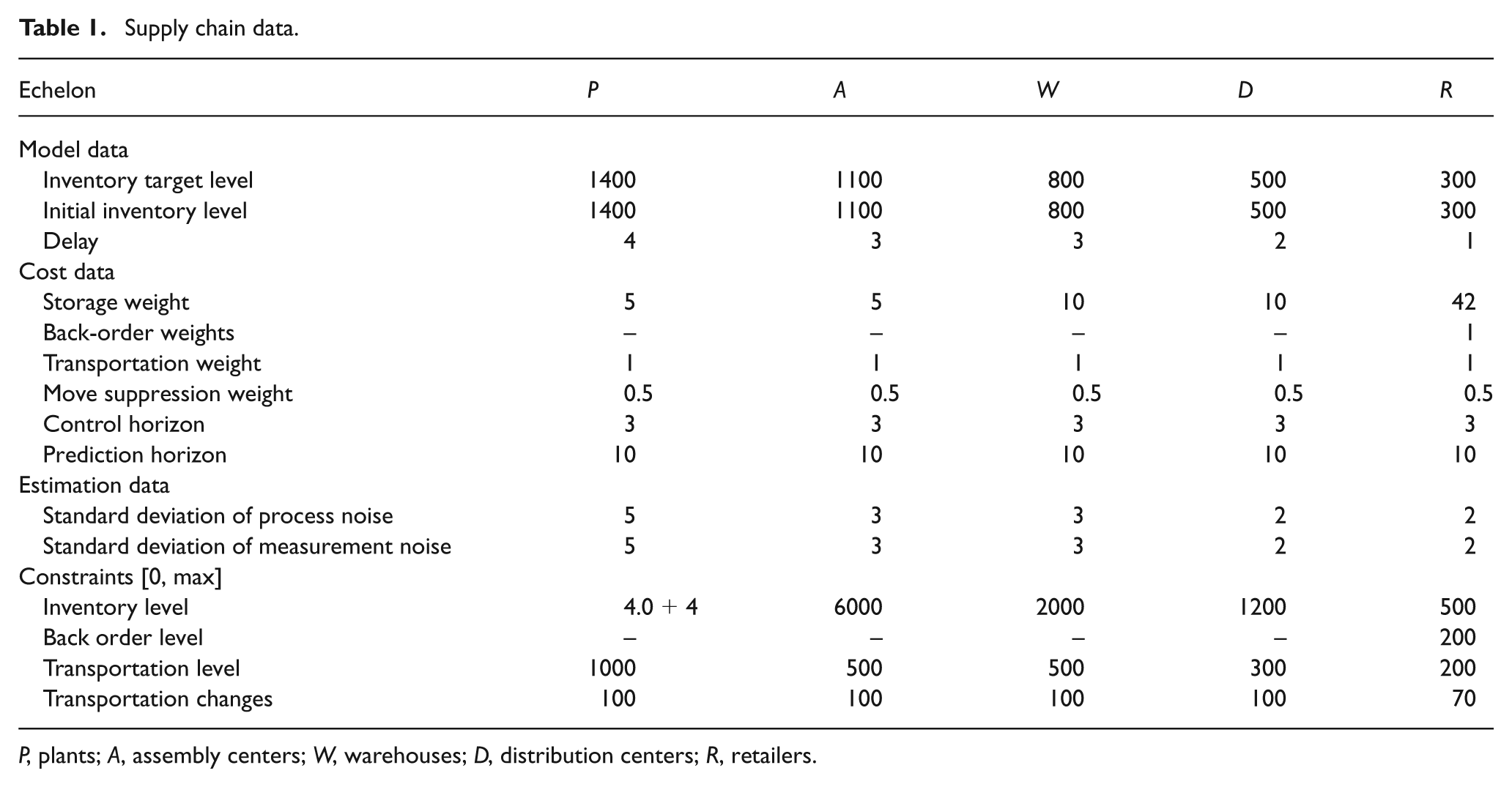
P, plants; A, assembly centers; W, warehouses; D, distribution centers; R, retailers.
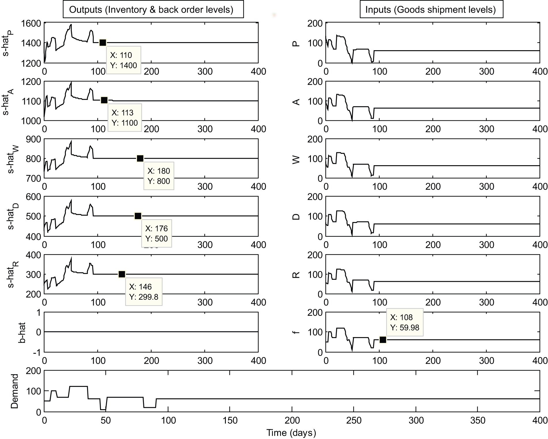
Firstly, must be said that all the state variables such as inventories are estimated by Kalman filter and indexed in the figures as ‘s-hat’ and ‘b-hat’ for different echelons. The base of the time is day and at first, the primary horizons define 10 days for prediction actions and 3 days for control actions. Figures 5–8 present the dynamic response of the supply chain to a deterministic step-like demand using the decentralized receding horizon control method. In Figure 5, the simulation is done without the move suppression effect and in Figure 6, this term is added to the performance index. In a comparison between the two figures, it is obvious that the suppression decreases change amplitude in the transferred products, settling times and input–output picks considerably. Use of the move suppression term can reduce the system speed. This slowdown can be seen in Figure 6, in which the rise times are reduced rather than the observations in Figure 5. Also, target tracking is improved using move suppression.
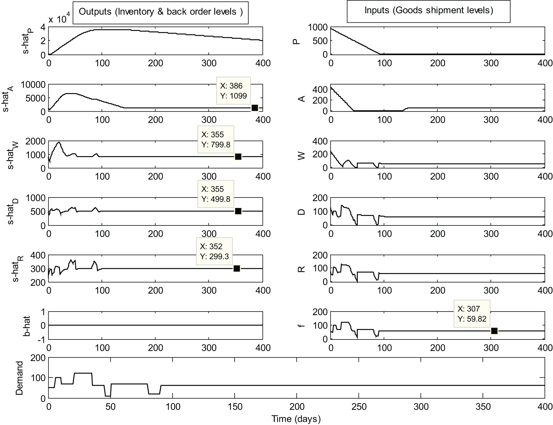
Dynamic response to deterministic demand without move suppression.
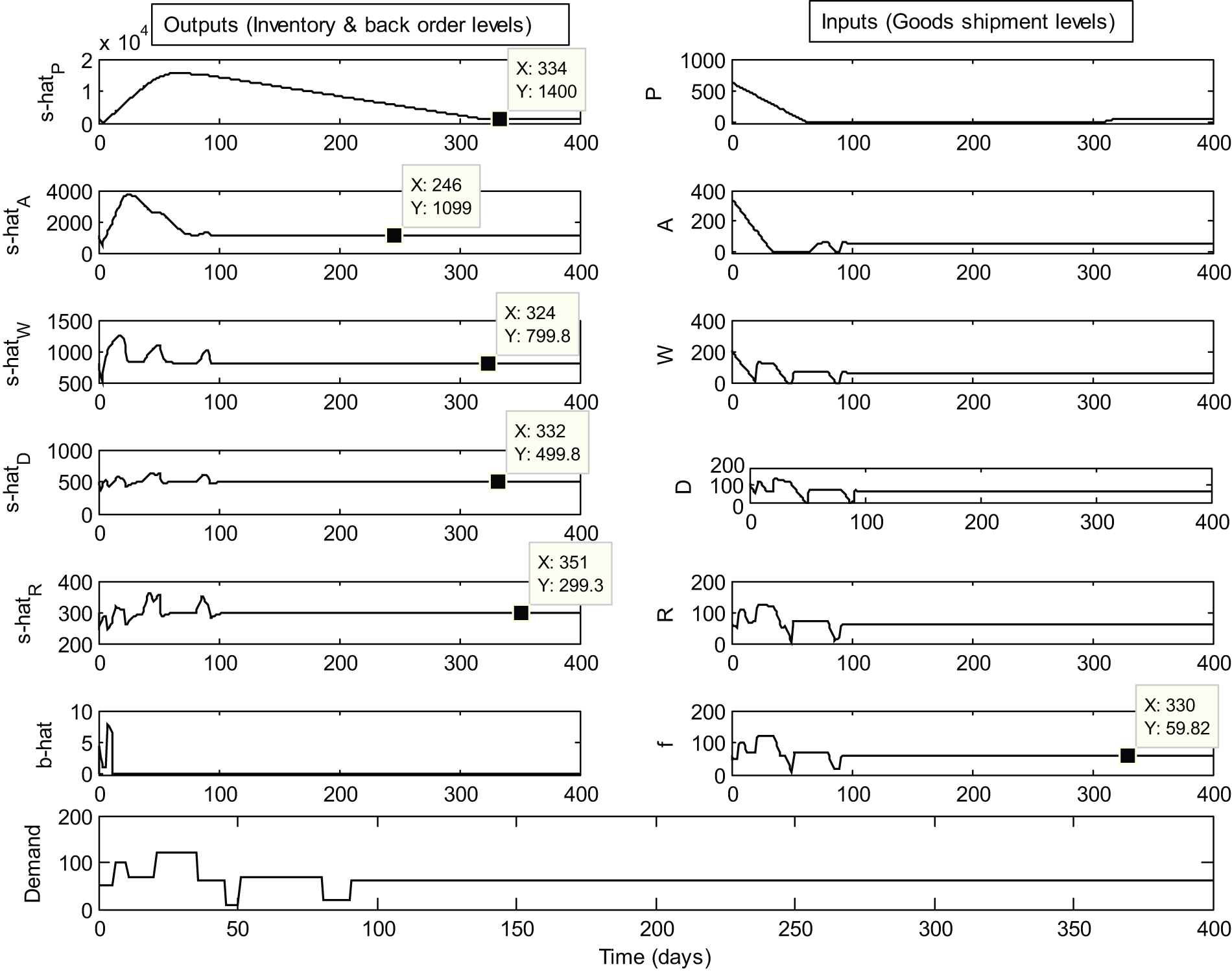
Dynamic response to deterministic demand with move suppression.
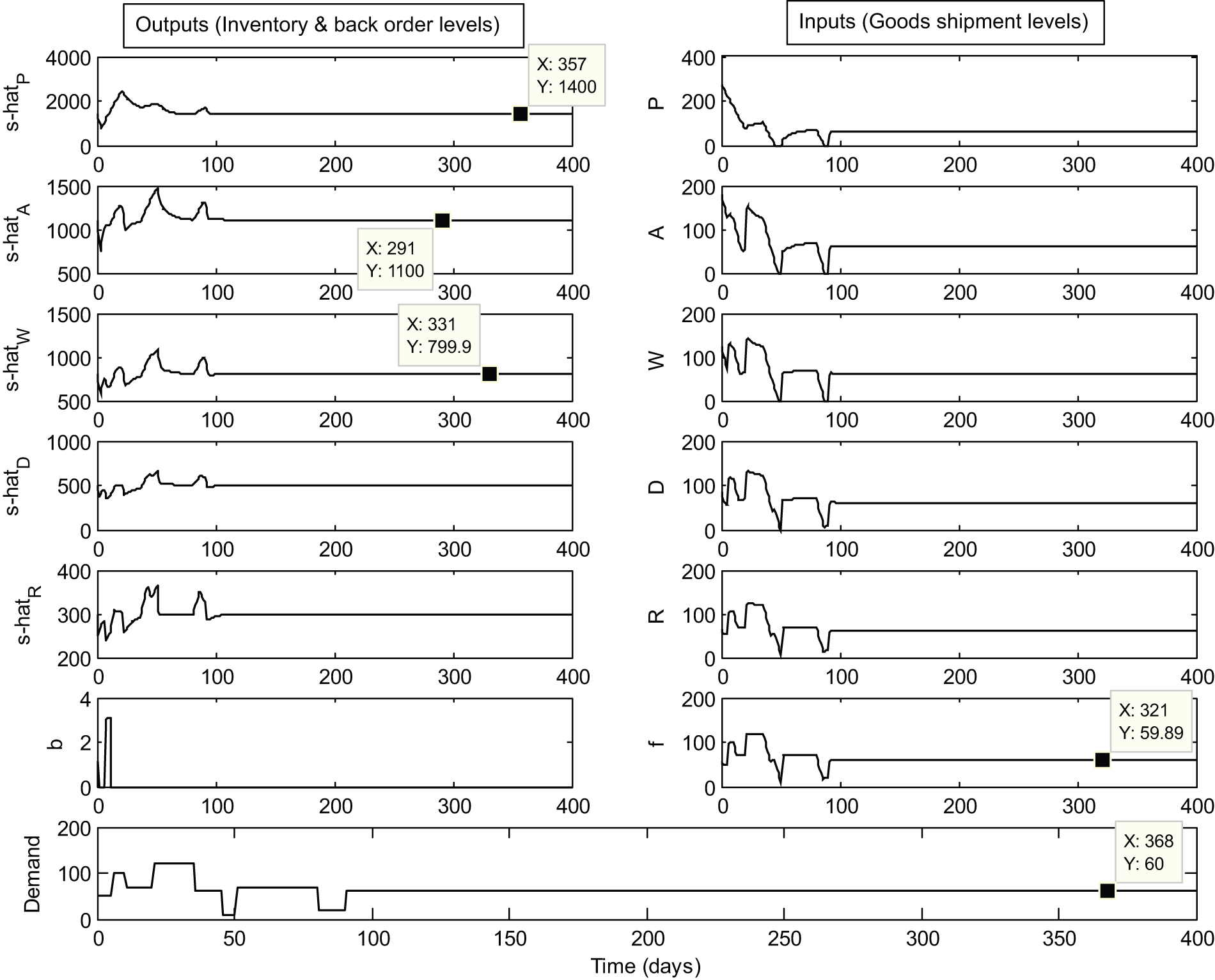
Dynamic response to deterministic demand with look-ahead scheme.
Dynamic response to deterministic demand with p=30 and c=6 days.
Another effect studied in the research is the look-ahead scheme, which uses all the predicted amounts of demands (measurable disturbances generally) over the prediction horizon, unlike the previous simulations, which just used the first array of predicted amounts and extended it throughout the horizon. As can be seen in Figure 7, the look-ahead scheme reduced the rate tracking of the inventory and the back orders, as well as the input and output peaks rather than that shown in Figure 6.
The length of control horizon and prediction horizon should be selected with regard to their effects on responses. As can be seen in Figure 8, a comparison with Figure 7 can be introduced, as the prediction horizon is upgraded to 30 days and the control horizon to 6 days. It can be said that the meeting time (settling times) in the tracking graphs can be reduced with increasing the size of the prediction horizon and the peak values can be more damped with increasing the size of the control horizon. Despite the merits of long horizons, they force higher computation loads on control systems corresponding the horizon amplitude.
As a result, with regard to Figures 5–8, a trade-off must be created between the tracking weights, the move suppression weights and the horizons to achieve lower cost and higher efficiency (demand fulfilment).
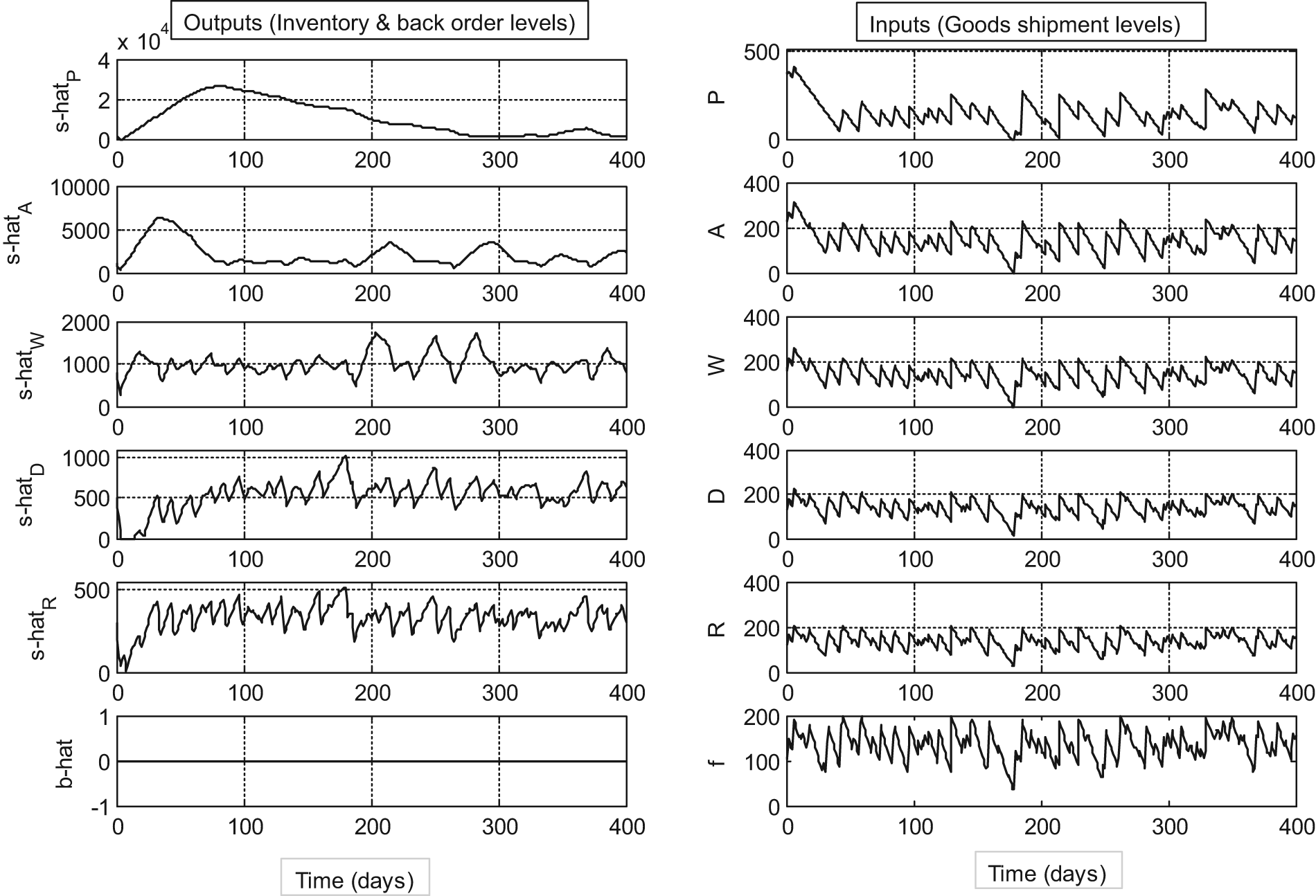
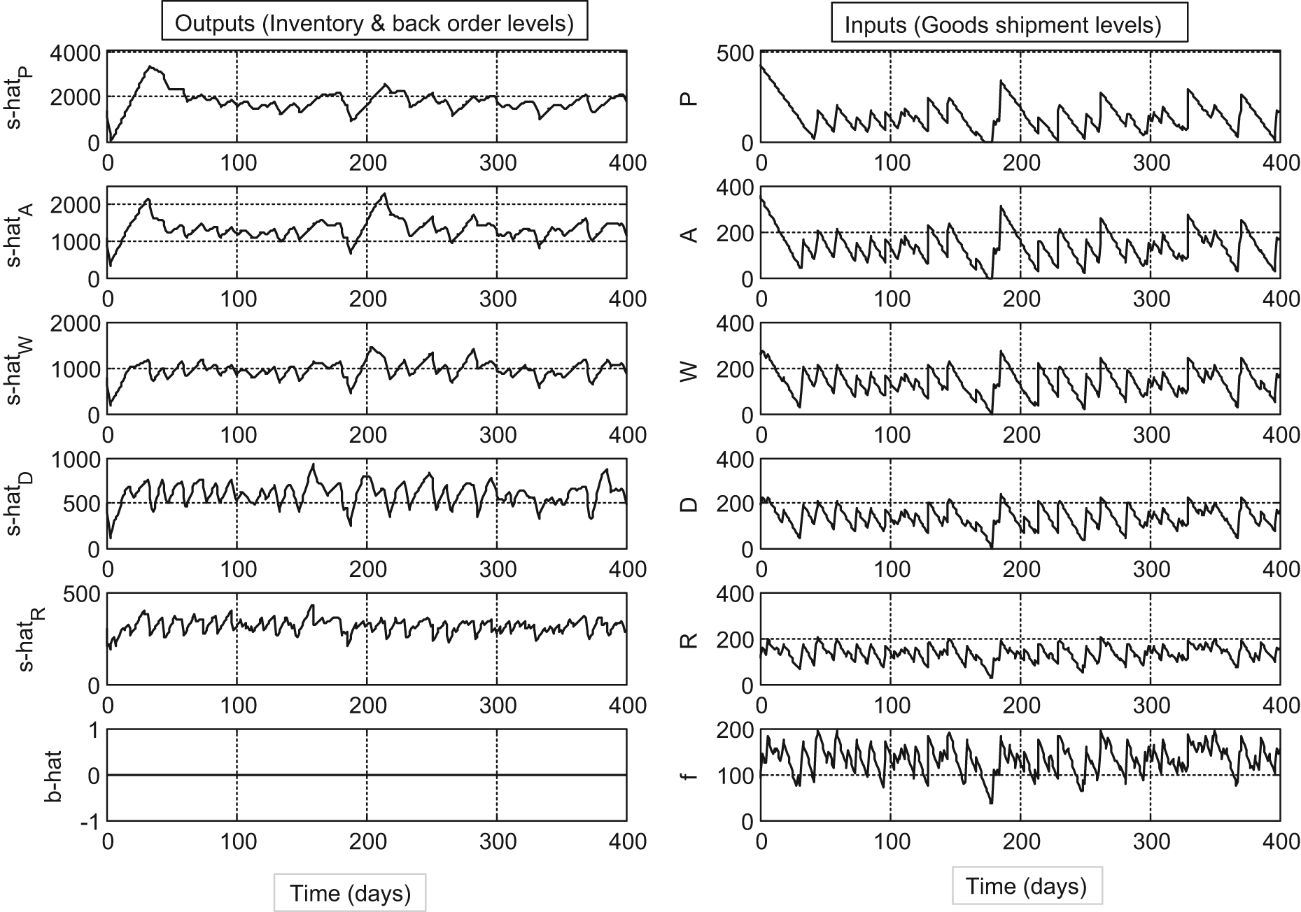
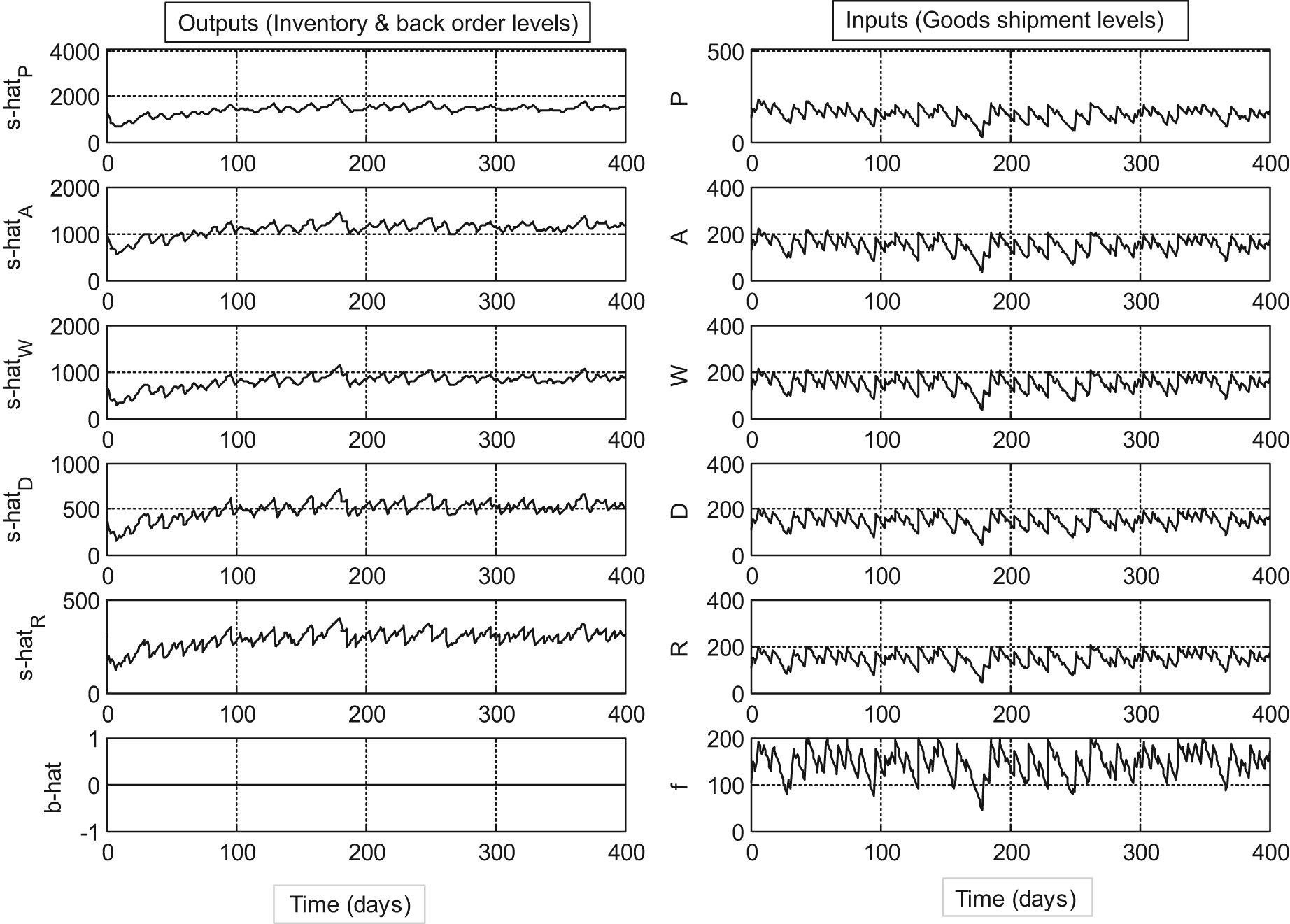
Figures 9–11 concern stochastic demands and are designed for p=25 and c=3 days because of the violent changes in demands. The mean stochastic demand over time is assumed as a uniform distribution of 1–200 product units.
Dynamic response to stochastic demand without move suppression with p=25 and c=3 days.
Dynamic response to stochastic demand with move suppression with p=25 and c=3 days.
Dynamic response to stochastic demand with move suppression with p=25 and c=3 days using centralized receding horizon control.
Figures 9 and 10 present a better study on the move suppression effect because they have large and multiple fluctuations in the demand. According to Figure 10, suppressing the input rates can omit a significant amount of fluctuations and improve the responses compared with Figure 9.
Figure 11 can be interpreted differently between the centralized scheme and the decentralized scheme. In the centralized receding horizon control, the dynamic responses are reformed in the fields of settling time, inventory tracking, transportation costs, customer satisfaction and so on. In addition to controlling hazards in the implementation as centralized, the computing time is greatly increased. The experiment is performed on a personal computer including core 2 duel CPU, 2.66 GHz and 4.00 GB RAM. With these qualities, the necessary times of simulation are 30 min for the centralized scheme and 10 min for the decentralized scheme, respectively. On the other hand, implementing a high dimension input is almost impossible for devices and forces a high risk of practical errors in comprehensive supervisory control.
Without a move suppression term, primary inventory levels are high and the back orders are zero, because there is no order accumulation. In this paper, lost orders are considered a part of demands, as
Conclusions
Supply chain management systems are large-scale systems and should be controlled in a decentralized form because of some practical advantages. These advantages include simplicity, time saving, lower computation cost, lower error risks, more safety and decreasing system input dimension by dividing into local subsystems, rather than the centralized control version. In this paper, a version of MPC based on a state space model named receding horizon control, because of its efficiency in applying constraints (inventory level, storage capacity and so on) and online adaption to severe changes (demands) using past information, is used as multi-agent control with a decentralized structure for supply chain management. Therefore, the decentralized model is simulated with the cooperation procedure and the efficiency is tested by simulation. These tests consider the effects of elements such as move suppression, the look-ahead scheme, changing the horizons and control centralization under deterministic and stochastic demands. Concerning the simulations, the move suppression term decreases the deviation of target levels (more robustness) and transported products, but instead reduces the dynamic response speed. This challenge can be resolved using accelerators such as local auxiliary classic controllers inserted as constraints or other innovative methods. Also, the look-ahead scheme and extending the horizon length improves the efficiency by decreasing output peaks and settling times. Finally, a simulation is shown to realize the performance of the centralized receding horizon control method. According to this simulation and its computation time, the advantage of centralized control in customer satisfaction and lower cost, and its disadvantage in time costs, are clear. Some future research in this field can be proposed as follows: the optimal merger of some nodes to increase the simplicity and decrease computation loads, define the horizon size for each echelon separately, consider uncertainty on the model and performance parameters, and design an accelerator for sluggishness treatment.
Footnotes
Funding
This research received no specific grant from any funding agency in the public, commercial, or not-for-profit sectors.
Nomenclature
A Assembly centres
b Back order
C Cost (performance index)
c Control horizon, day
D Distribution centres
d Demand
δ Time interval
f Delivered product
i Node
i’ Upstream node
i” Downstream node
id Desired for node i
KE Kalman estimator
L Transportation delay, day
l Transported product
MPC Model predictive control
N Covariance of measurement noise
P Plants
p Prediction horizon, day
Q Covariance of process noise
R Retailers
S Suppliers
s Product inventory (stock)
T Time
t Time, day
u Unfulfilled order (lost order)
υ Measurement noise
W Warehouses
w Weight