






Abstract
A novel design method of decoupling internal model control is proposed for non-square processes with multiple time delays that are often encountered in complicated industrial processes. The method can obtain a realizable decoupling controller of non-square processes with more inputs than outputs by inserting some compensated terms, which are derived analytically. Meanwhile, based on the relative normalized gain array, an equivalent transfer function matrix is introduced to approximate the pseudo-inverse of the process transfer function matrix, which makes the design of decoupling internal model control simple and easy to calculate. Filters are added to the control structure to improve the robustness. Simulation results have proved the effectiveness and reliability of the proposed method.
Keywords
Introduction
In a complex industrial production process, it is always necessary to use multiple controlled variables and multiple manipulated variables to describe a controlled system, and we often encounter a class of systems in which the number of input variables and output variables are usually not equal, which are known as non-square systems. Although non-square processes in industry are very common, the literature on controller design of non-square system is still sparse. A traditional approach towards the control of non-square processes is to square up or square down the systems to square systems through adding or deleting appropriate inputs (manipulated variables) or outputs (controlled variables). Thereafter, most well developed control strategies for square systems (where the number of inputs and outputs are equal) can be applied directly.
However, adding inputs or outputs to be measured can be costly, while removing inputs or outputs will lead to a poor performance because of the information that is neglected and may even make the system unstable through the possible introduction of right half plane (RHP) poles. Therefore, a promising approach to the above problems is to design a controller for the original non-square system (Morari et al., 1985). Treiber and Hoffman (1986) have showed that the performance achieved by using the full non-square model of a vacuum distillation unit is superior to the result obtained by employing a square subsystem, and the non-square system is illustrated to possess a better control character and stronger robustness compared with any of the possible squared-down systems designed by an independent robust controller (Loh and Chiu, 1997).
Internal model control (IMC) has been proved an effective method to resolve time-delay and decoupling problems (Garcia and Morari, 1982, 1985). On the basis of the IMC principle, the design of a decoupling controller for a square system is generally based on the inverse matrix of original system (Liu et al., 2006). However, considering non-square processes, IMC cannot be applied directly, as it cannot obtain the traditional sense of inversion. In addition, it is also difficult to select the non-minimum phase part of a transfer matrix with multi-delay for optimal performance. To overcome these questions, a modified IMC method for non-square processes with multiple time delays and right-half-plant zeros is proposed (Chen et al., 2008). In order to improve dynamic quality and robustness of non-square systems with first-order time delay, the IMC method is used to design Smith delay compensation to compensate for shortcomings caused by static decoupling, and also overcome the impact of the model error on the system performance by model approximation (Chen et al., 2011). Because IMC is a method of realizing the controller design, relying heavily on the inverse or generalized inverse of process model, it is important to research a simple and easy method to calculate the inverse or generalized inverse.
In this paper, a novel design method of decoupling IMC is proposed for non-square processes with different time delays. The method can realize decoupling of non-square processes by inserting some compensated terms, which are derived analytically. Meanwhile, an equivalent transfer function (ETF) matrix was used to approximate the pseudo-inverse of the process transfer function matrix, which makes the design of decoupling IMC simple and easy to calculate. The simulation results show the effectiveness of the proposed method. However, it is worth mentioning that the proposed method is specific to plants with more inputs than outputs, as IMC is based on the assumption of perfect control, but for systems with more outputs than inputs, perfect control is in the least-square sense. Obviously, the proposed method cannot be applied to control it perfectly; how to achieve the control of that should be further studied.
The design of decoupling internal model control
The decoupling IMC structure
A block diagram of IMC control structure is shown in Figure 1, where
where
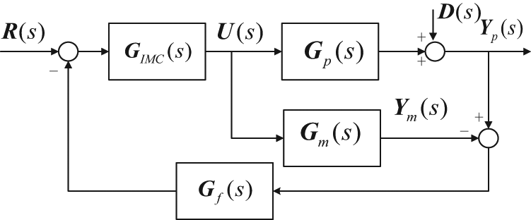
Structure of internal model control (IMC).
The design of internal model controller
The design procedure of the controllers
From Figure 1, the closed-loop transfer matrix
Assuming
According to the traditional IMC theory, the system is decoupled if and only if
Then, from (3), the decoupling internal model controller can be written as:
It is obvious that
First, determine
where
Next, choose the appropriate
where
Then (3) becomes to
Here,
where
The design of feedback filter
In industry, model inaccuracies widely exist, and thus it is necessary to include filters in the feedback signals, in order to make the system maintain the original performance. When uncertainty exists in the control system, the system robust stability can be guaranteed by increasing the value of control parameter
For the
where
Using the cut-frequency of the filter as a third of the frequency of these oscillations,
Internal model controller design based on equivalent transfer function
The internal model controller designed by the above procedure usually has a complicated expression, especially when the system dimension is high. In this section, the ETF method is employed to find a simple description for
For multivariate systems, ETF refers to open equivalent transfer function of a loop in the case of other loops being closed. Then how to obtain the ETF model is an important issue. Relative normalized gain array (RNGA) was provided by Xiong et al. (2007), and using the array, the change of steady state gain, time constant and delay time can be obtained when other loops are closed, and then the approximate model of ETF can also be obtained based on original transfer function (Shen et al., 2010). In this paper, it is expanded to non-square processes.
Equivalent transfer function for non-square processes
For non-square processes, by assuming that the process is under perfect control, relative gain array (RGA) and RNGA is extended to non-square multivariable systems (Chang and Yu, 1990). The non-square relative gain (NRG) is defined as the ratio of the open-loop gain to the closed-loop gain. Then the open-loop gain is easy to obtain by the transfer function, while the closed-loop gain is not that straightforward. Under the assumption of ‘perfect control’, which is to say the designed controller makes all outputs
Similar to the square RGA, the NRG and the NRGA are defined as
and
respectively. In form (12),
To describe the dynamic properties, the normalized gain
In the above expressions,
The non-square RNGA (NRNGA) can be written as
Furthermore, the relative average residence time
where
From (13)–(15), NRARTA is calculated by
where ⊙ indicates element-by-element division.
Previous investigations have shown that almost all industry processes can be simplified to a first-order-plus-time-delay (FOPTD) model. For simplicity, consider the FOPTD model for a transfer function
The average residence time is formed as
Then the changes of transfer function elements when other loops closed can be uniquely determined. An ETF element when other loops are closed can be approximated by a transfer function element and has the same form as the open-loop transfer function element, where the steady state gain, the time constant and the time delay are scaled by NRGA, NRNGA and NRARTA, respectively, i.e.
where
The relationship between equivalent transfer function array and system transfer function matrices
For square systems, Xiong et al. (2007) established the relationship between
For a non-square system, the non-square dynamic RGA (NDRGA) is defined as
Under the assumption of perfect control, the NDRGA can also be calculated by
Comparing (24) and (25):
Taking the transpose of both sides of (25), we obtain
From the above, substituting (26) into (11), the decoupling internal model controller is calculated by
By using ETF, the design of
Furthermore, carrying on the analysis on the impact of ETF model approximation, when adding decoupling controller, the closed-loop transfer matrix
Assume the best loops pairing are i–i. First considering the diagonal elements, to describe them clearly, we obtain the further expansion of (28)
where
where
Then, considering off-diagonal elements, it can be expressed that
It has been proved that
Taken together, for the best control effect, both conditions of (30) and (32) are expected to be established. However, if that is impossible, it needs to meet the constraint (32) first of all. Then update the time delay
Robust analysis and performance index
As a matter of fact, modelling errors and system uncertainties are inevitable and cannot be ignored when modelling a real plant, and the present of uncertainties usually causes instability and poor performance of control systems, thereby leading to very complex dynamical behaviours. It is necessary to analyse the robust stability of the proposed control system, and in this subsection, we analyse the system robustness.
As for the standard assumptions in robustness analysis, the nominal IMC system is stable. Suppose that the control system with the additive uncertainty is denoted by
where
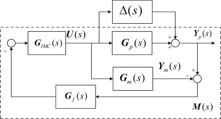
System with additive uncertainty and its
For convenience and for analysing robust stability, the general
According to the robust stability theorem (Morari and Zafiriou, 1989), the proposed control system is robustly stable for
where
If
Simulation results
Two plant models are considered to demonstrate the effectiveness of the proposed design methods.
Example 1
Consider the shell control problem with three inputs and two outputs (Ogunnaike and Ray, 1979). The transfer function matrix is given as
The open-loop gain, time constant, and time delay of the system are given as
A simple calculation gives
which results in the following ETF parameters
Substituting these ETF parameters into the original transfer function matrix, the ETF matrix is obtained as
According to Equation (10), the form of
In view of the robustness and response time, filters are selected as
Thus, the final decoupling controller is obtained as
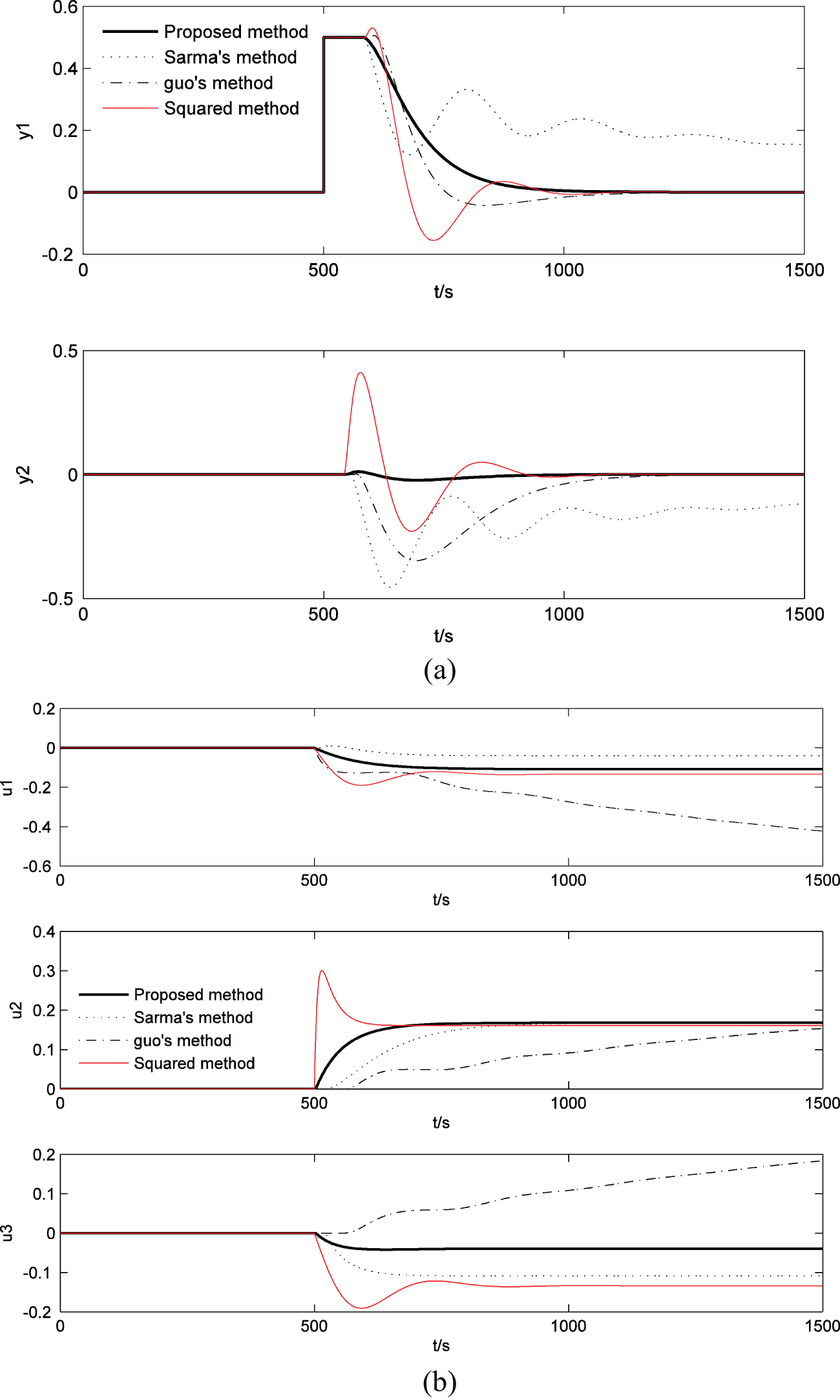
At a perfect matching of a process plant and model, the set-point responses of the system for a step change in
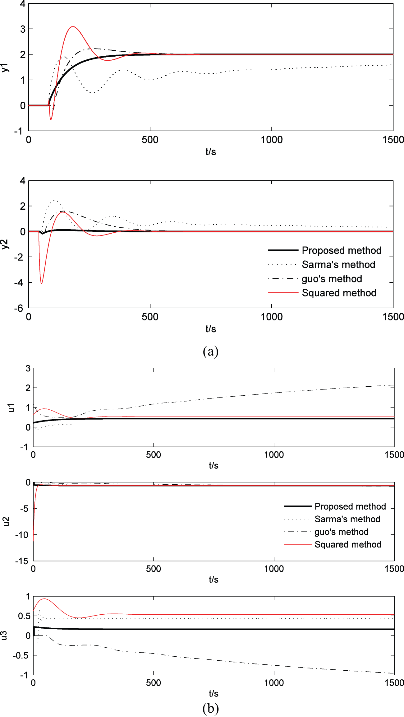
Set-point responses for perfect model for a step in
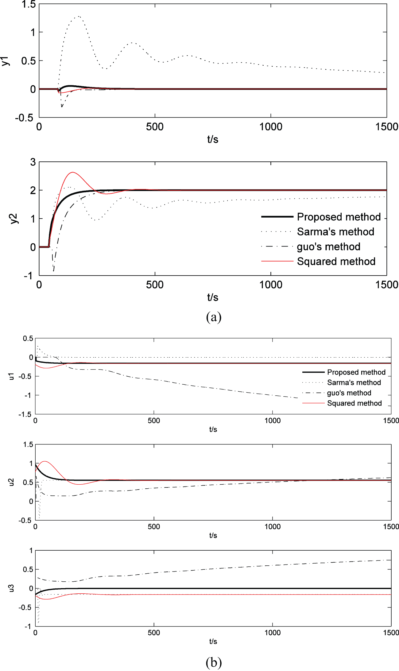
Set-point responses for perfect model for a step in
Disturbance responses for a 0.5 step in
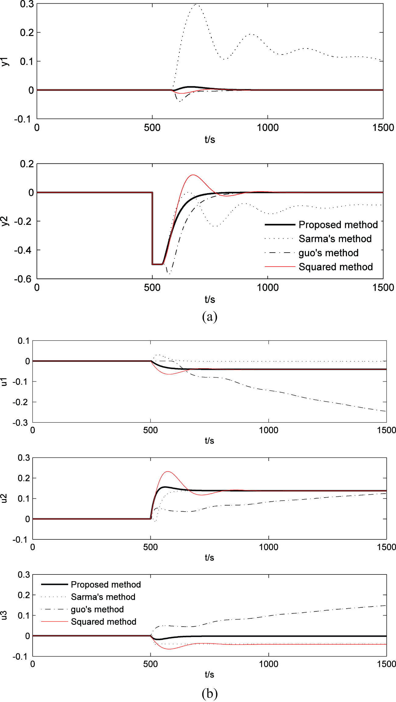
Disturbance responses for a −0.5 step in
It can be seen from the simulation results that the method proposed in this paper makes two outputs nearly decoupled and driven to their steady-state values. Compared with those given by the other three methods, the proposed method shows smaller overshoot, faster tracking features and disturbance rejecting performance.
In order to verify the robustness of the proposed method, we increase the gains and the dead times of the process elements by 20%, and, conversely, the time constants are decreased by 20% and the process becomes:
Under the condition of the set-point and the controller parameters being constant, the set-point responses are shown in Figures 7 and 8. From the results, we conclude that the proposed method still offers good tracking features and strong robustness in the case of the given perturbation.
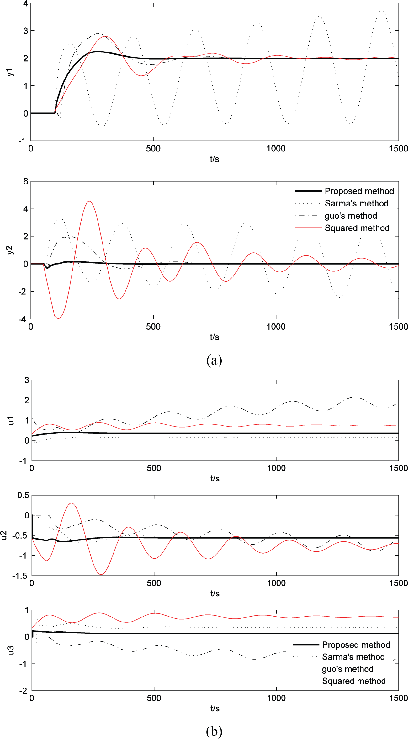
Set-point responses for the given perturbation for a step in
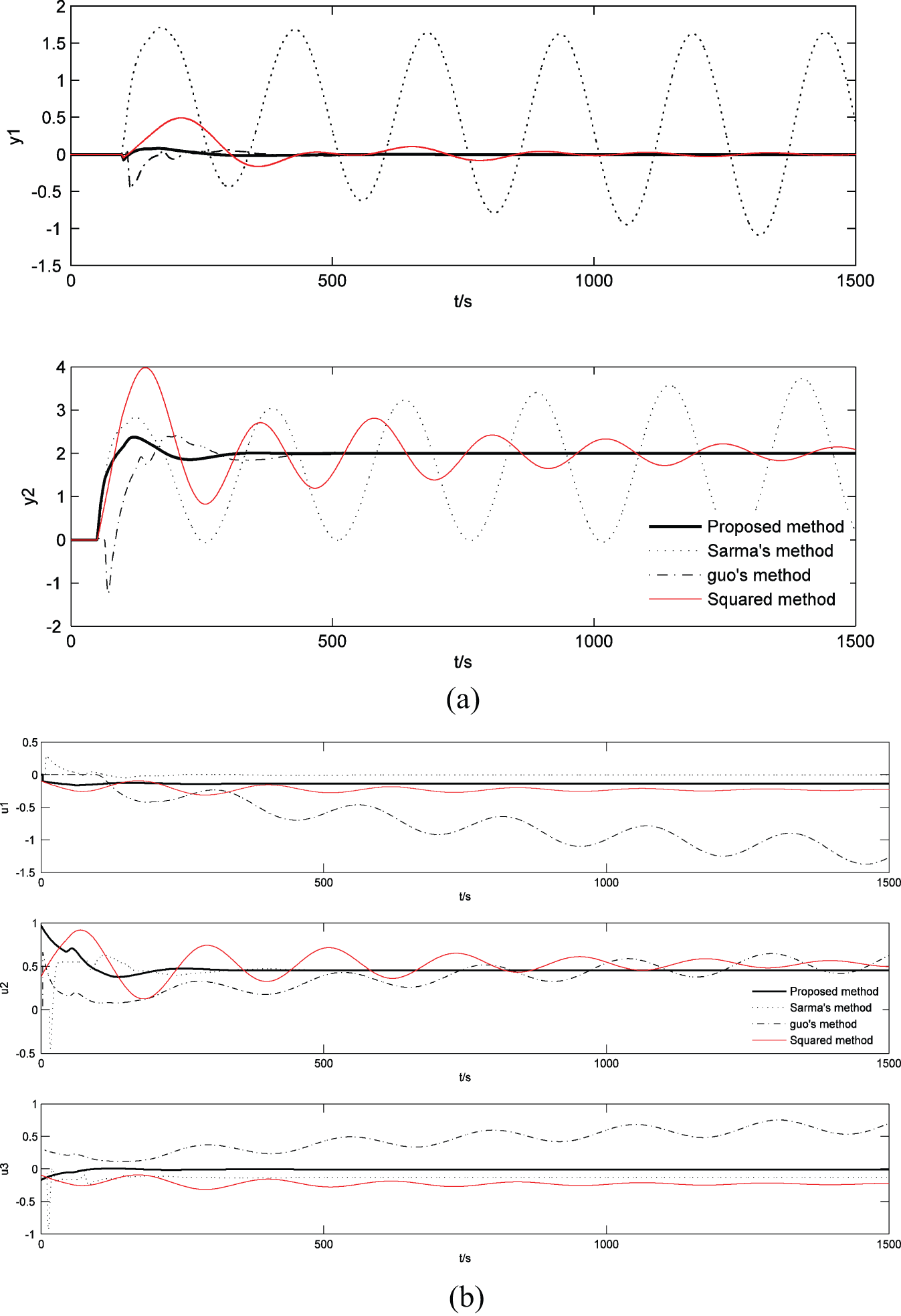
Set-point responses for the given perturbation for a step in
To evaluate the decoupling result and dynamic performance comprehensively, the integral of squared error index (ISE; Lin et al., 1999), which considers the sum of the ISE values in response and interaction, is chosen as the performance index. To make a performance comparison among these four methods, the matching ISE values corresponding to the set-point responses and the mismatching with perturbations are shown in Table 1. From the ISE values, it is observed that the proposed method gives slower ISE values and shows no apparent variation during process model mismatches. This is a clear indication that the method proposed in this paper demonstrates good robustness.
Integral of squared error index (ISE) values when process plant matches and mismatches with process model.
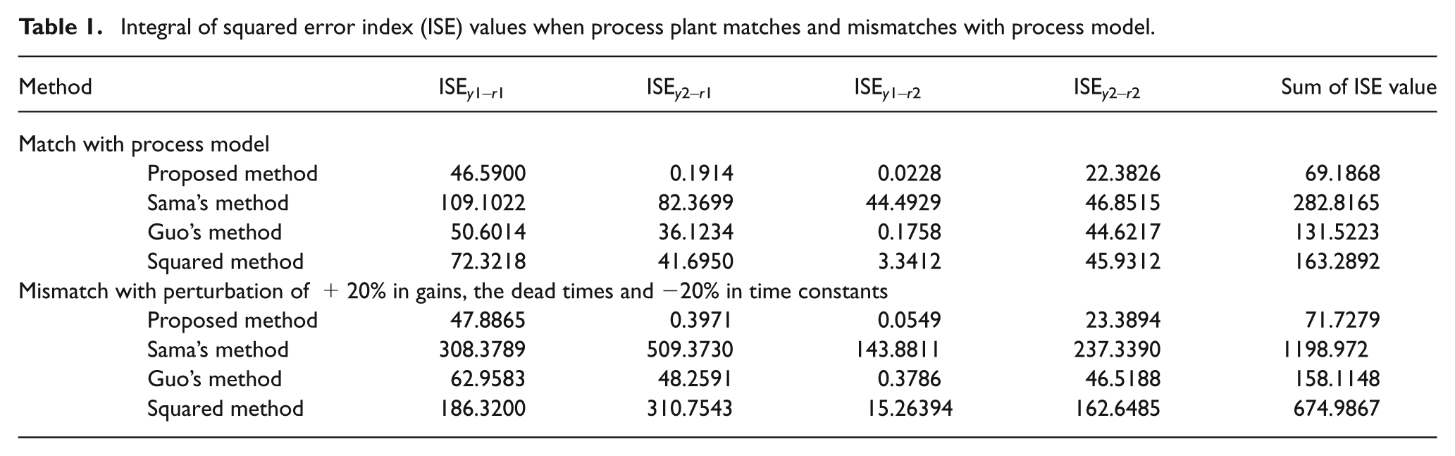
Judging from the simulated curves of these figures, we can conclude that the proposed controller works well. Furthermore, the tracking performance is better and the speed of response is faster than the other methods when there is a model mismatch.
Example 2
Let us consider another example of a hot oil fractionator with four inputs and two outputs (Ogunnaike and Ray, 1994)
Then, the final decoupling controller is obtained as
To show the improvement of our method, the centralized PI controller
where
The steady-state gain matrix is obtained as
The corresponding pseudo-inverse is obtained as:
Thus, the controller transfer function matrix can be written as
To obtain good closed-loop performances, the tuning parameters are selected as
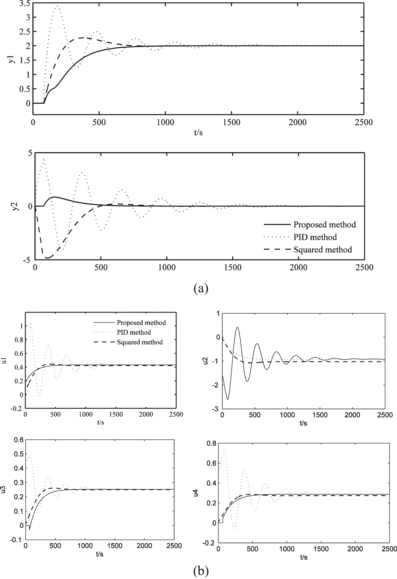
Set-point responses for perfect model for a step in
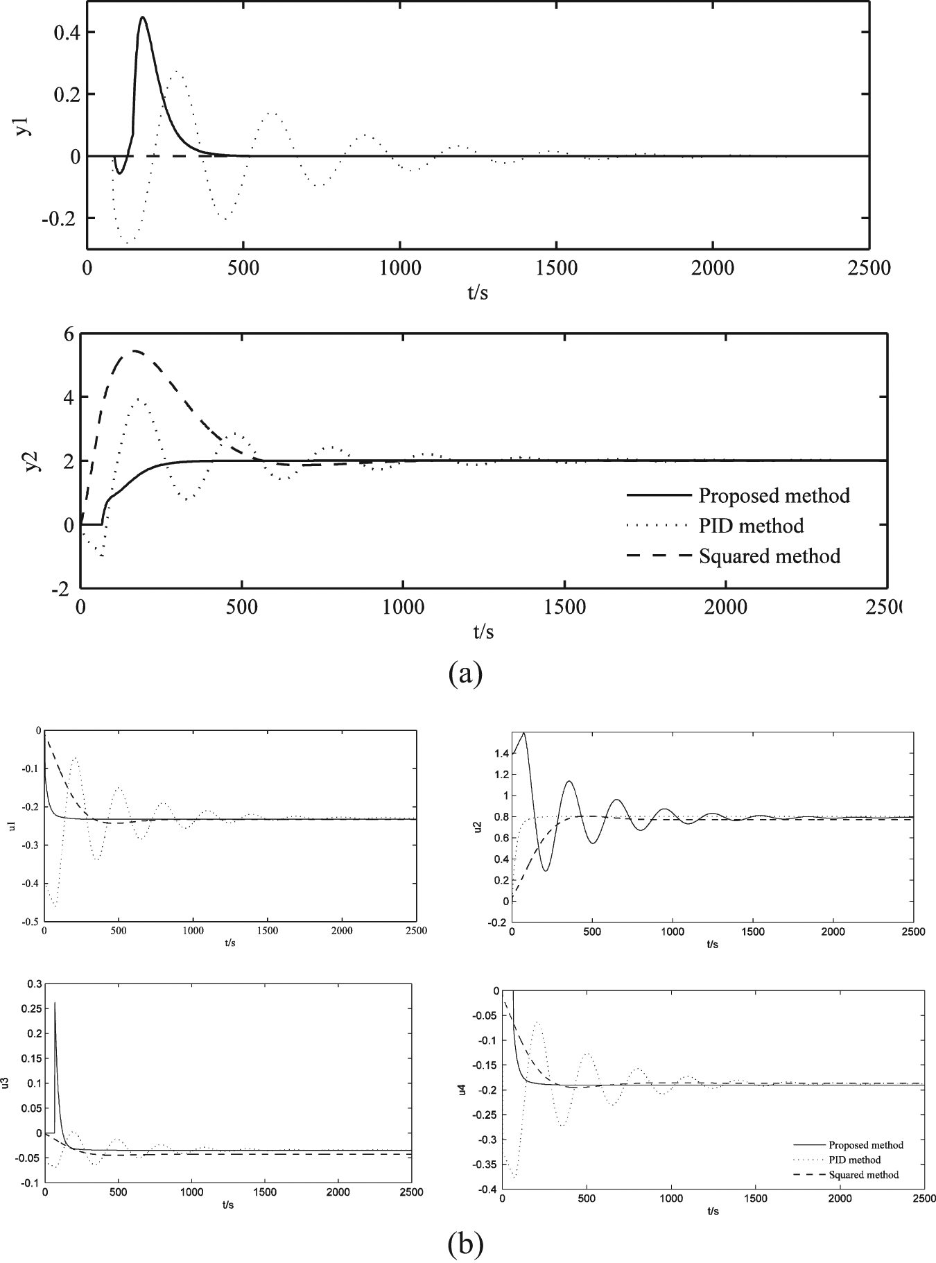
Set-point responses for perfect model for a step in
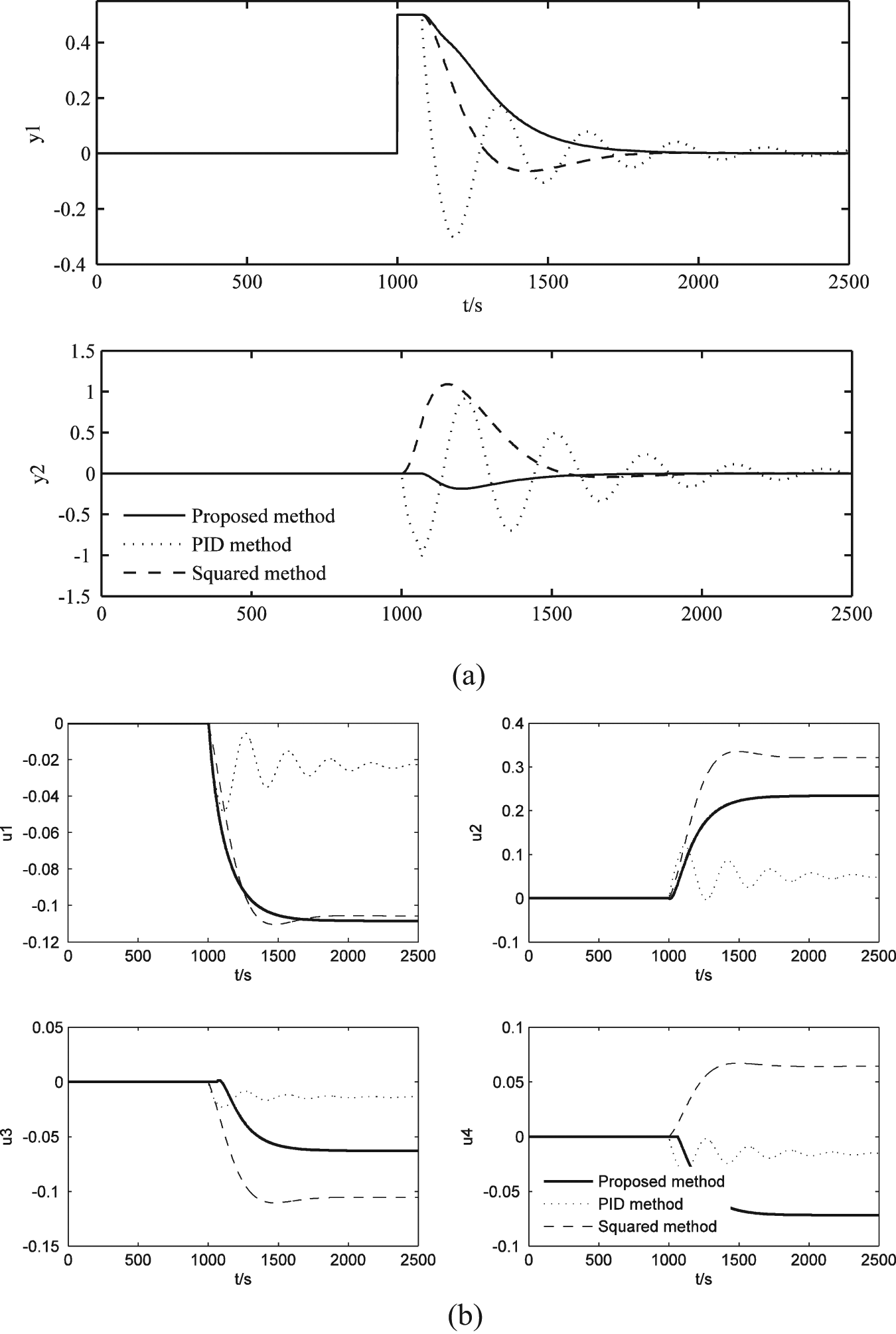
Disturbance responses for a 0.5 step in
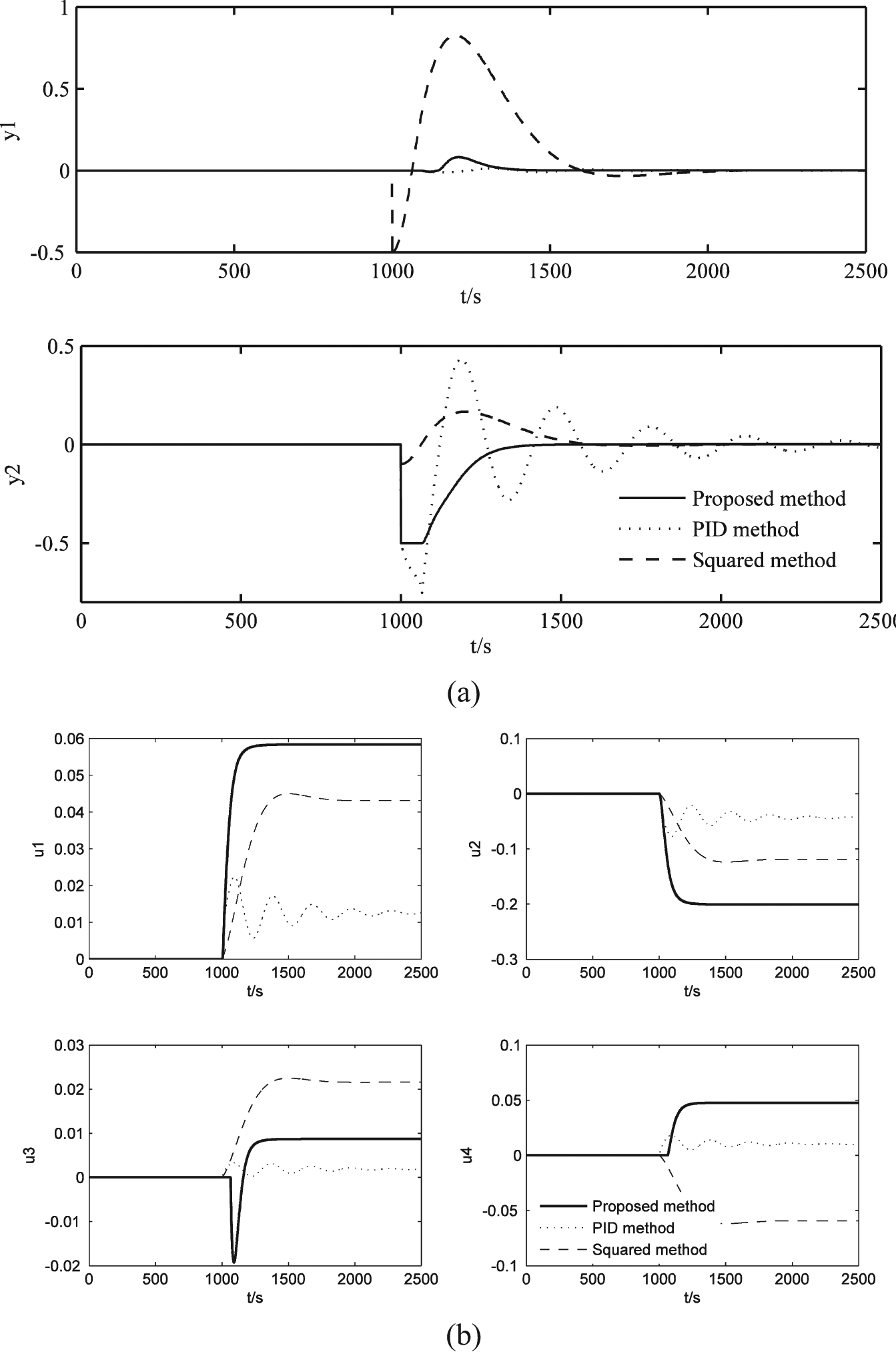
Disturbance responses for a −0.5 step in
In order to verify the robustness of the proposed method, we increase the gains and the dead times of the process elements by 20%, and, conversely, the time constants are decreased by 20%, and then the process becomes:
When the model is mismatched, the set-point responses are shown in Figure 13. It can be seen from the simulation results that the method proposed in this paper has a smaller overshoot, faster tracking features, less interaction, better anti-interference performance, and is driven to steady-state values under the given perturbation.
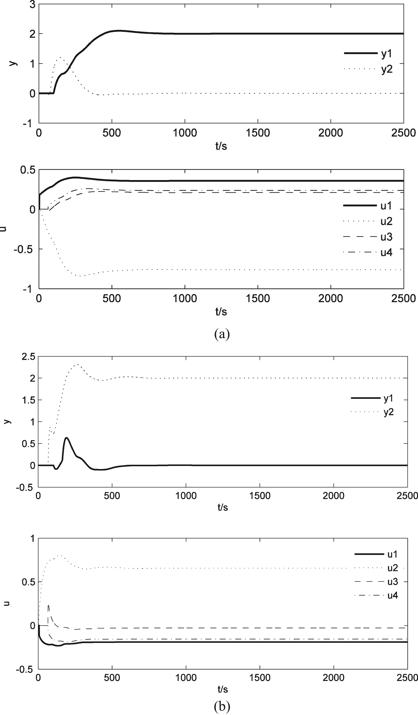
Set-point responses for the given perturbation: (a)
From the simulation curves of these figures, we can conclude that the proposed controller has better tracking performance and faster response speed than the PID control method and squared method whether the model is matched or not.
As can be seen from the above two examples, the proposed IMC based on ETF not only has a good performance on tracking given value and overcoming disturbance, but also has good decoupling and control quality both in model match and mismatch cases. Moreover, the designed controller is easy to compute and realize. In brief, the designed controller works well, and can achieve a certain control level.
Conclusion
A new method for decoupling IMC, focusing on a class of non-square stable processes with multiple time delays, has been presented in this paper. The method in this paper proceeded from the desired diagonal transfer function matrix of the system, based on the stability and realizability, to design a compensator, and then obtained the final decoupling internal model controller based on the pseudo-inverse. Furthermore, the calculation of the pseudo-inverse based on ETF matrix was very simple, straightforward and easy to understand, and the ETF element has the same form as the open-loop transfer function element, so the decoupling internal model controller has a simple form. The results of simulation have illustrated that our approach gives better control performance and robust performance than other methods. However, there are several limitations of our present study, which should be taken into consideration. as possible limitations of the study, it should be noted that all our results were obtained under the assumption of perfect control, which barely exists in practical engineering. Without question, for the design of multi-variable control systems, there often exists conservation by using the proposed method. Another limitation is that we did not extend this method to non-square systems with fewer inputs than outputs, while the experiments were directed only toward another kind of non-square system with more inputs than outputs, probably because it is difficult to achieve good results in cases where the number of control variables are fewer than output variables. An additional research issue that should be tackled is how to design IMC controllers for non-square systems with fewer inputs than outputs, which we are currently planning.
Footnotes
Acknowledgements
The authors are grateful to the anonymous reviewers for their valuable recommendations.
Funding
This work was partially supported by the financial support of the National Science Foundation of China (grant number 61273132) and the National Grand Fundamental Research 973 Program of China (grant number 2007CB714300) and partly by the Automation Institute Beijing University of Chemical Technology.