






Abstract
This paper proposes two novel methods for fault detection in non-linear processes. These methods apply a Gaussian process (GP) to model the underlying process, and then the extended Kalman filter (EKF) and square root cubature Kalman filter (SCKF) are used to detect faults. Accordingly, two approaches called the Gaussian process–extended Kalman filter (GP-EKF) and Gaussian process–square root cubature Kalman filter (GP-SCKF) are proposed. The most important characteristic of these proposed methods is that there is no need for an accurate model of the system. Therefore, these methods are considered non-parametric approaches of fault detection in non-linear systems. To illustrate the performance of these algorithms in fault detection, they have been used in a continuous stirred-tank reactor system (CSTR). Both proposed methods are able to detect sensor faults at an early stage.
Keywords
Introduction
Progress in different sciences and industries make their applied systems bigger, more complicated and more intelligent. In these systems, the occurrence of faults is inevitable. As designing healthy systems with optimal performances is one of the most basic concerns of industrial system designers, a fault detection and diagnosis unit is an inseparable part of industrial and dynamic systems. Among fault detection and diagnosis systems, the best is the one that can detect faults within the shortest possible time and with the least loss.
Until now, several fault detection methods have been proposed for non-linear systems (Blanke and Schröder, 2003; Chen and Patton, 2012; Zhang D et al., 2013). One of the most successful approaches is the Kalman filter (KF), which has been used in dynamic systems (Doraiswami and Cheded, 2012; Safarinejadian et al., 2013; Liu J et al., 2014; Wang and Qi, 2015). One of the main disadvantages of the KF is that its application is restricted to linear systems, whereas physical systems are non-linear, inherently; therefore, the standard Kalman filter is unable to detect the faults in these systems. Consequently, the non-linear version of KF that is known as the extended Kalman filter (EKF) is used to detect faults of non-linear systems (Efimov et al., 2011; Foo et al., 2013; Zhang X et al., 2013). In this method, due to the linearization error that exists in the filter implementation, the state estimation does not show sufficient accuracy. Therefore, the present method is unable to perform well, especially in those systems that are strictly non-linear, or in those systems that need higher terms of the Taylor series expansion for the linearization of process and measurement equations. To overcome these problems, another method known as the unscented Kalman filter (UKF) has been proposed for fault detection of the non-linear systems (Cao and Ayalew, 2015; Liu H et al., 2014; Lu et al., 2014; Masoumnezhad et al., 2015). In this method, a set of sample points known as sigma points are used for the mean and the covariance estimation. Using these sigma points in the state estimation can reduce the computational complexity. However, there is more than one free parameter in the implementation of UKF and setting these parameters to reach the desired estimation is rather difficult to apply. Moreover, the performance of the filter may be interrupted in higher dimensions because, which is one of the regulative free parameters of UKF, may be negative (Julier et al., 2000). Due to the mentioned UKF drawbacks in detecting the fault of non-linear systems, the cubature Kalman filter (CKF) is proposed (Zarei and Shokri, 2014). The CKF that has the same computational load as UKF is able to generate more accurate first and second moments than UKF (Arasaratnam, 2009; Mu and Cai, 2013).
In the above-mentioned methods, an accurate model of the system is needed to detect faults. However, an accurate mathematical parametric model is never accessible, as considering all aspects of the system model is difficult; besides, some factors of modelling involved such as friction are often neglected to make the task easier. Therefore, most non-linear systems either have no parametric model or have an approximated model. In both cases, parametric methods of fault detection are neither useful nor have a desired performance. To address these advantages, researchers have proposed a non-parametric method known as the Gaussian process (GP) as a substitution for the model of the system (Rasmussen and Williams, 2006; Shi and Choi, 2011). GPs have been used in the fault detection of dynamic systems (Juricic and Kocijan, 2006). Recently, a new algorithm for the non-linear state estimation has been proposed by combining the GP and parametric methods (Deisenroth et al., 2012; Ko and Fox, 2011).
In this paper, two new methods of fault detection, called the Gaussian process–extended Kalman filter (GP-EKF) and Gaussian process–square root cubature Kalman filter (GP-SCKF), are proposed for fault detection of non-linear systems. These methods have been developed by combining the EKF and the square root of the CKF with GPs. The main advantage of the proposed approaches is that there is no need for an accurate model of the system. Furthermore, these methods have a sufficient accuracy in generating the residual signal. Moreover, by applying the square root of CKF, this method has less computational complexity and is also more stable numerically (Hao et al., 2012). Consequently, applying a highly accurate method, which has some lower computational complexity, can generate a residue that is sensitive to the faults of the system and can detect them in the minimum possible time.
The present study is structured as follows: the statement of the problem and the required necessities of presenting the proposed algorithms are described in the next section. Then, the proposed algorithms and the methods of their application in fault detection are presented. Simulation results are given and, finally, the conclusion is provided.
Problem statement
The Gaussian regression model
The main characteristic of GPs is their flexibility in modelling, as they can model the unknown functions when there is an uncertainty in the function. By using training data, a GP is able to learn the noise imposed on the function and to smooth parameters (Rasmussen and Williams, 2006). More information can be found in Safarinejadian and Kowsari (2014), Shi and Choi (2011), and references therein.
The GP is briefly introduced in the following. The non-linear regression model is given as:
where
In a GP, a form that is selected as the covariance function is the square exponential (SE) covariance function, which is determined by using Equation (3) (Rasmussen and Williams, 2006).
In this equation,
The conditional density
and its corresponding conditional mean and covariance are as follows:
where
The exponent on the right-hand side of Equation (7) has the below square shape:
where
Expanding Equation (9) results in:
By substituting Equations (8) and (11) with
Therefore, the conditional density of
In the following, the mean and the covariance functions of the posterior distribution over function f are computed based on Lemma 1. The joint distribution of values of observations y and the predicted values of function
Learning hyper parameters
In order to calculate a suitable GP, which can approximate the unknown function f appropriately and optimally, GP parameters or those parameters that are in the kernel function must also be determined optimally. To fulfil this aim, the
The logarithmic term of (19) can be written as:
The optimization problem is carried out by optimization technique such as the conjugate gradient. Partial derivatives, which are needed for optimization, are given as:
Proposed algorithms for fault detection
In the next subsection, combining the EKF and SCKF with the GP are described. Then, the computational complexity of the proposed algorithms will be investigated. Finally, these algorithms will be used to detect faults of the system.
The combination of the Gaussian regression model with the extended Kalman filter and the square root cubature Kalman filter
The main aim of this subsection is to model
Here, X is the matrix of states,
In this equation,
By substituting this distribution in the EKF and SCKF:
In the measurement update step of Bayesian filters, the aim is to determine
The distribution of function
The prior density of
However, by applying the GPs, considering the fact that the below functions are Gaussian integrals:
So
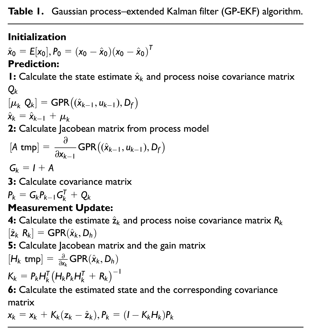
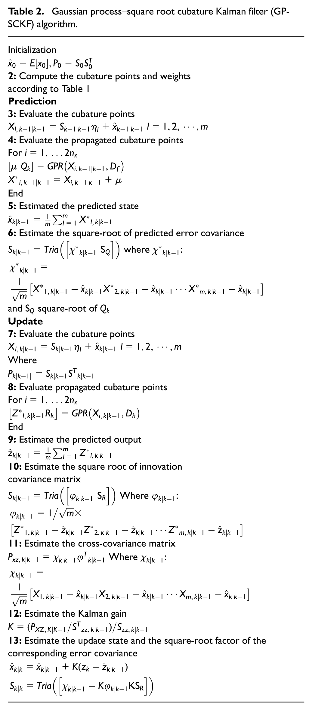
In order to describe GP-EKF and GP-SCKF, the steps of these algorithms are shown as Tables 1 and 2.
Gaussian process–extended Kalman filter (GP-EKF) algorithm.
Gaussian process–square root cubature Kalman filter (GP-SCKF) algorithm.
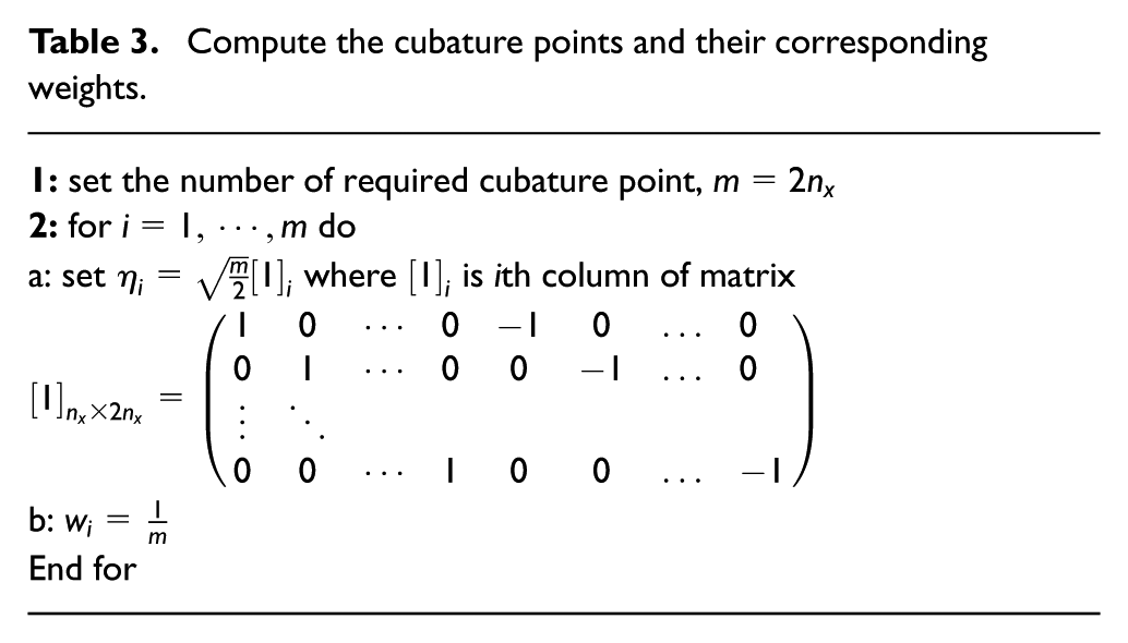
The cubature points and their corresponding weights can be calculated as presented in Table 3.
Compute the cubature points and their corresponding weights.
An investigation into the computational complexity of GP-EKF and GP-SCKF
In the time update and measurement update steps, the GP-EKF and the GP-SCKF are similar to their corresponding filters or the EKF and the SCKF. Substituting GPR with the unknown functions of the process and the observation is their only difference. Therefore, in this section only the computational complexity arisen from substituting GPR in SCKF is being investigated. At each step, the computational cost is shown by C. In the proposed method, the computational cost divided into the kernel cost
The GP-SCKF requires the computation of one mean for each cubature point; besides, in each step of performing the GP-SCKF algorithm, one covariance must also be calculated.
For more accurate analysis, the computational complexity of
Furthermore, it must be considered that
Finally, the linearization of GPs needs computing the Jacobin of kernel functions along with
Therefore, for every output dimension, the Jacobin complexity of the kernel function is equal to
Fault detection in non-linear systems
Assuming that there is a fault in the measurement sensor, the total system can be represented as:
where
Residual generation
The first step in the fault detection process is generating a signal, which is sensitive to the fault and is able to show the fault at the early stages. The simplest residual signal is defined as:
where
The residual analysis
Ideally speaking, the residue is zero if there is no fault in a system; otherwise, the residue is non-zero. In this case, the residual analysis is defined as:
However, in many systems, the residue is non-zero even at fault-free conditions. Therefore, the decisive function that is written in Equation (37) is not an appropriate residual analysis. To analyse the residual properly, it is possible to define a statistical decisive function as:
where
In selecting
Simulation results
To show the performance of the two suggested algorithms and to compare their performances, the implementation and the simulation results of the GP-EKF and the GP-SCKF will be explained as follows. The studied scenario is on a continuous stirred-tank reactor (CSTR).
As the CSTR systems transform raw materials into valuable chemicals, they are the most important part of many chemical, biochemical, polymer and petroleum processes. They can operate at low or high temperatures, in batch, fed batch or continuous mode.
The CSTR is widely used in many chemical plants. Due to changes in process parameters, the accuracy of final product can be reduced. In order to obtain an accurate final product, the faults occurring in the CSTR during the chemical reaction need to be diagnosed. If not, the faults may lead to degradation of the performance of the system
The process and measurement equation of this system is as follows:
where
Steady state parameters of continuous stirred-tank reactor system (CSTR).
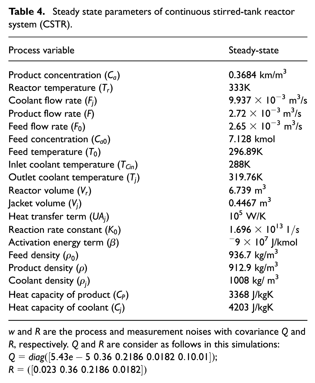
w and R are the process and measurement noises with covariance Q and R, respectively. Q and R are consider as follows in this simulations:
In these simulations, 500 random points have been selected for the training data set. The simulation results have been tested after 50 times of performing Monte Carlo simulation on 50 random data.
State estimation
To show the performance of GP-EKF and GP-SCKF and also to check the accuracy of these algorithms, the root mean square error (RMSE) of these methods for 50 Monte Carlo runs has been calculated and results are shown in Figures 1 and 2, and Table 5. The accuracy of the GP-SCKF method is better than the GP-EKF in state estimation as seen in Table 5.
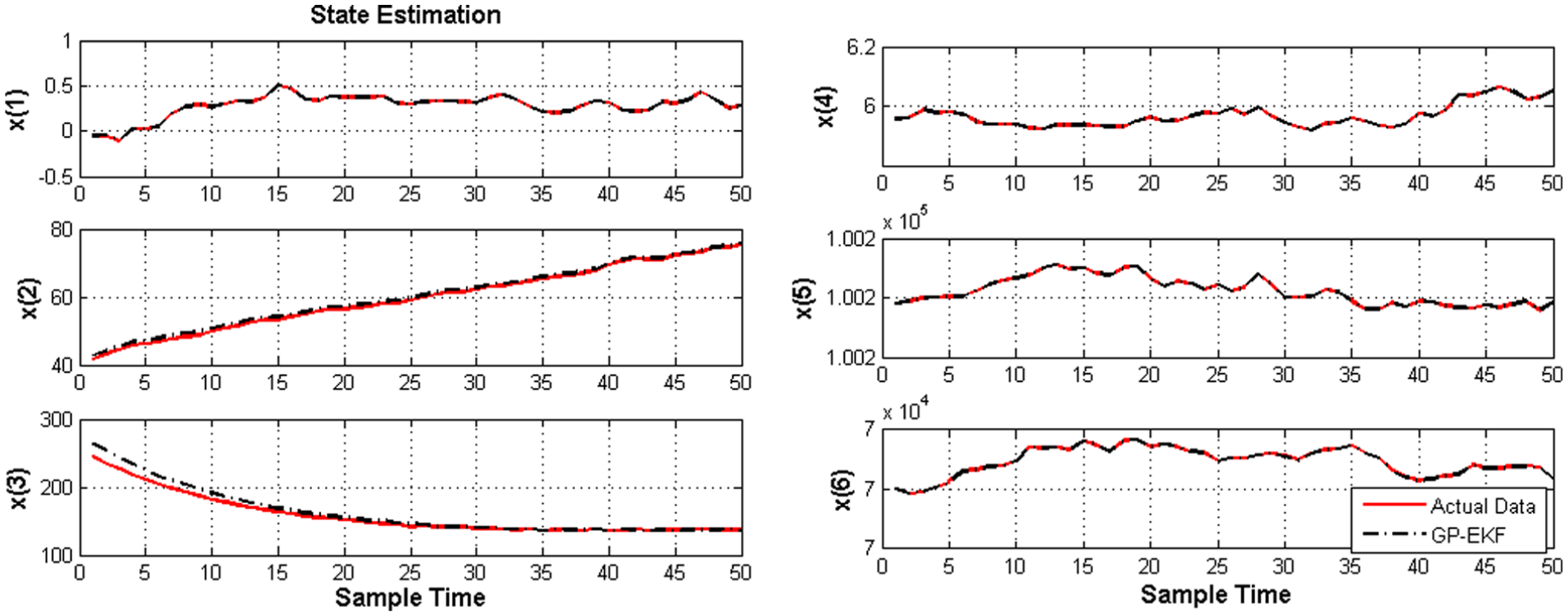
State estimation by Gaussian process–extended Kalman filter (GP-EKF).
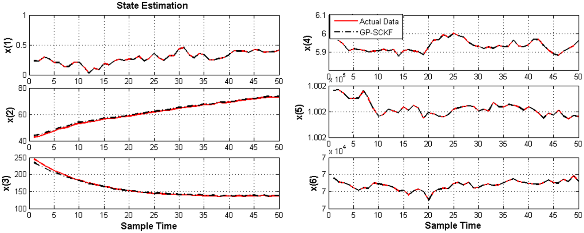
State estimation by Gaussian process–square root cubature Kalman filter (GP-SCKF).
Root mean square error of Gaussian process–extended Kalman filter (GP-EKF) and Gaussian process–square root cubature Kalman filter (GP-SCKF) in 50 Monte Carlo simulations.

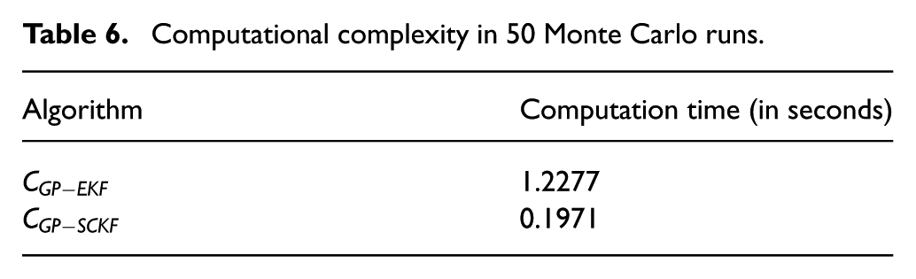
A comparison between the computational complexities of the two algorithms is shown in Table 6. In the table, it can be seen that the computational complexity of the GP-EKF algorithm is approximately six times more than the computational complexity of the GP-SCKF algorithm.
Computational complexity in 50 Monte Carlo runs.
Fault detection
To show the performance of these methods in non-linear fault detection, three kinds of faults in the sensor of the system has been analysed. These faults are known as abrupt, incipient and intermittent, and all are considered additive faults. In these simulations,
The additive fault detection process by applying the GP-EKF and GP-SCKF algorithm
In this simulation,
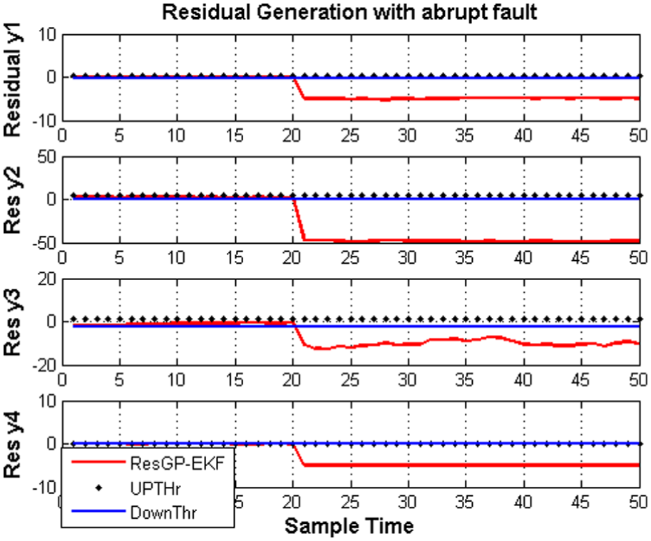
The residue generation by Gaussian process–extended Kalman filter (GP-EKF) (abrupt fault).
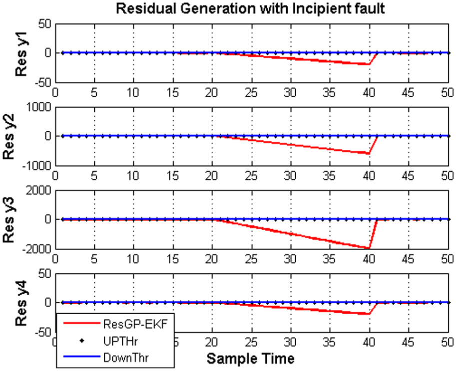
The residue generation by Gaussian process–extended Kalman filter (GP-EKF) (incipient fault).
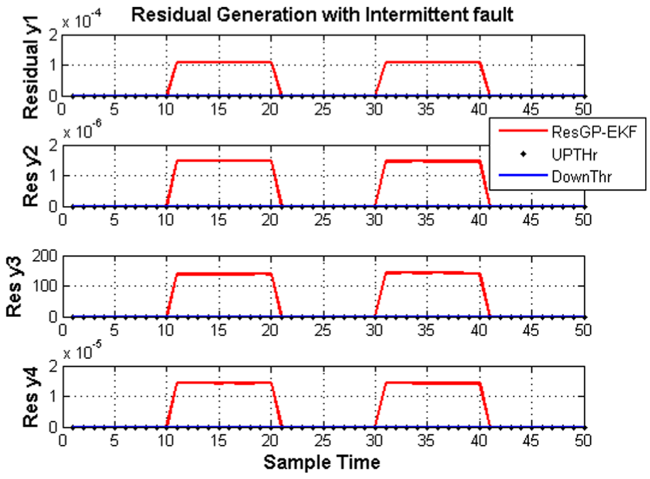
The residue generation by Gaussian process–extended Kalman filter (GP-EKF) (intermittent fault).
Figure 6 indicates the residual signal that is generated by the GP-SCKF algorithm when an abrupt fault has occurred within the system. Figure 7 shows the system residual signal when an incipient fault is imposed upon the system and Figure 8 manifests the residual signal generated by the GP-SCKF algorithm when there is an intermittent fault in the system. As observed in Figures 6, 7 and 8, the GP-SCKF algorithm can detect the fault as well as the GP-EKF algorithm. However, the main advantage of the GP-SCKF algorithm is that it has fewer mathematical computations than the GP-EKF algorithm Moreover, unlike the GP-EKF algorithm, it is possible to use the GP-SCKF algorithm in strictly non-linear systems.
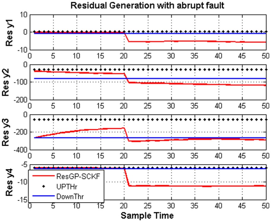
The residue generation by Gaussian process–square root cubature Kalman filter (GP-SCKF) (abrupt fault).
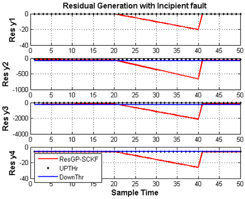
The residue generation by Gaussian process–square root cubature Kalman filter (GP-SCKF) (incipient fault).
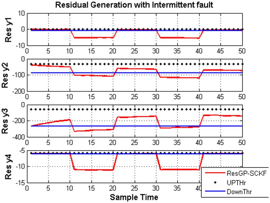
The residue generation by Gaussian process–square root cubature Kalman filter (GP-SCKF) (intermittent fault).
The delay times of these methods for fault detection have been shown in Table 7. According to this table, occurrence of fault can be detected in the shortest time or early stage.
Delay time of fault detection.
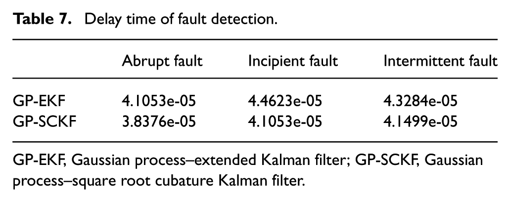
GP-EKF, Gaussian process–extended Kalman filter; GP-SCKF, Gaussian process–square root cubature Kalman filter.
Non-additive fault detection process by applying GP-EKF and GP-SCKF algorithms
In the proposed fault detection methods, a residual signal will be obtained from the difference between measured output and estimated output (
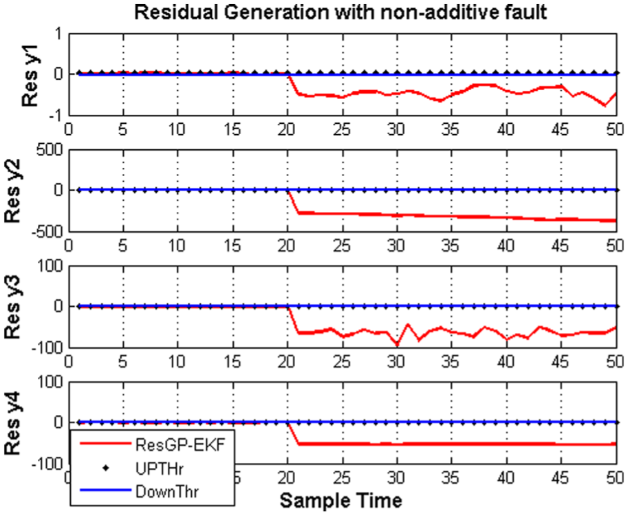
The residue generation by Gaussian process–extended Kalman filter (GP-EKF) (multiple fault).
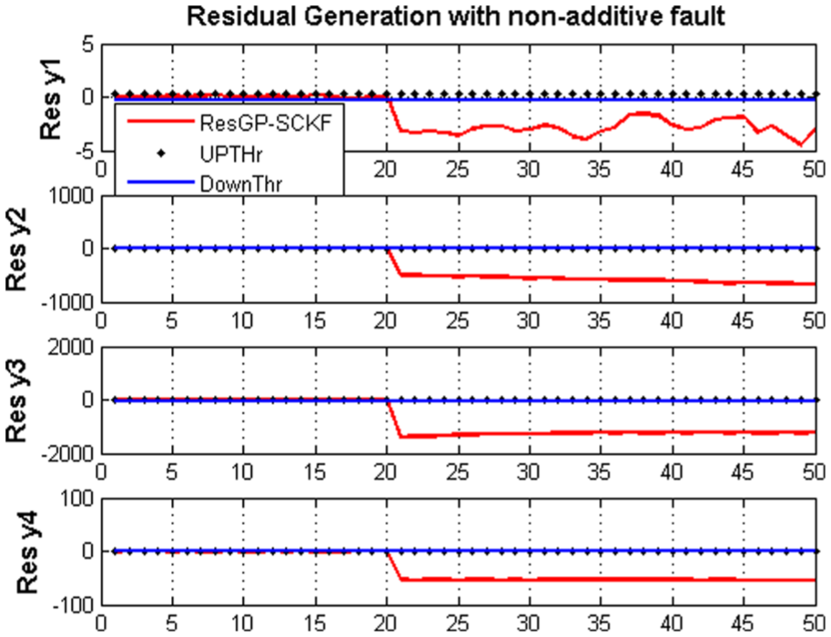
The residue generation by Gaussian process–square root cubature Kalman filter (GP-SCKF) (multiple fault).
Discussion
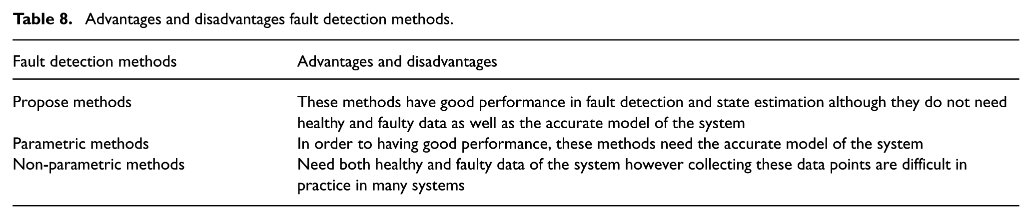
It is illustrated that without needing an accurate model of the system, the state estimation can be done with appropriate accuracy. The simulation results show that GP-SCKF is more accurate than the GP-EKF. Furthermore, it has lower computational complexity compared with GP-EKF. Therefore, it can detect faults faster than the GP-EKF. A brief comparison between the fault detection methods is available in Table 8.
Advantages and disadvantages fault detection methods.
Conclusion
In this paper, two new methods are proposed for the purpose of non-linear fault detection systems. The algorithm of the proposed methods, their computational complexity, advantages and disadvantages have all been analysed; furthermore, these methods have applicably been tested to find out their strength in the fault detection and fault diagnosis domain. The most important advantage of these algorithms compared with the previous ones is that they do not need to use accurate equations of the system and have high accuracy in generating the residual signal. Ultimately, in order to implement the proposed method in detecting the fault of non-linear systems, a comparison has been made between these algorithms. The results obtained from this comparison have proved the superiority of the GP-SCKF algorithm, especially due to its low complexity of computations and high accuracy.
Footnotes
Appendix
Conflict of interest statement
The author(s) declared no potential conflicts of interest with respect to the research, authorship, and/or publication of this article.
Funding
The author(s) received no financial support for the research, authorship, and/or publication of this article.