A ripple-based maximum power point tracking method for three-phase grid-connected photovoltaic inverter

Abstract

As a prevailing solar energy utilization equipment, the three-phase grid-connected photovoltaic (PV) inverter is widely operated in partially shaded conditions and thus tends to generate multiple local maximum power points on its power-to-voltage and current-to-voltage characteristic curves. In order to identify the global maximum power point (GMPP) quickly and precisely, this paper proposes a ripple-based maximum power point tracking method. It aims to perform the optimization of tracking using the segmented scanning of DC-side voltage. An improved adaptive perturb and observe (AP&O) method is introduced to maximize the solar conversion and to increase working stability. This method applies a hybrid model of fixed and variable step-size perturbation to restrain the fluctuation of PV-side voltage. It belongs to a two-stage GMPP tracking method. That is, when environmental factors such as irradiance and temperature change quickly PV power fluctuates sharply. Correspondingly, the AP&O method tracks the latest maximum power point (MPP) with a large fixed-step voltage reference command. When the PV power fluctuates smoothly under a slow environmental change rate, the algorithm applies multiple small and variable step-size voltage perturbations to vibrate round the location of GMPP. Simulation and experimental results show that this method improves the efficiency of the PV inverter tracking performance. In addition, the stability of DC bus voltage is guaranteed, and the operational stability of the photovoltaic power generation system is improved.

Keywords

Photovoltaic inverter maximum power point tracking single-stage system adaptive perturb and observe partially shaded conditions

Introduction

Efficient utilization of solar energy has been a hotspot in the power generation field. As an important component in a photovoltaic power generation system (PPGS), a photovoltaic (PV) cell is an energy conversion source in the whole system, varying output power since it is vulnerable to the impact of external environmental factors (i.e. irradiance, ambient temperature and local shadowing) (Fusco and Russo, 2013; Ishaque and Salam, 2013; Reisi et al., 2013). In order to obtain a stable power output from the PV cell, common practice is to apply the maximum power point tracking (MPPT) method to track the maximum power point (MPP) of PV arrays so as to keep the inverter at its highest conversion efficiency. According to the nature of a PV cell, when it is under uniform irradiance its output has a single maximum power point (i.e. a unique global maximum power point (GMPP) exists). When the cell is affected by changing environmental conditions – varying temperature, irradiance, shadows, array allocation, clouds, shielding by nearby buildings, etc. – the output of a PV cell has multiple extreme points (Patel and Agarwal, 2008).

Literature review and comparison

Most research on MPPT under local shadowing conditions focus on the following aspects. (1) Location (Ishaque et al., 2014): how to discriminate extreme power points accurately and distinguish GMPPs from local maximum power points (LMPPs), and locate to GMPPs precisely. (2) Tracking speed (Ghoddami and Yazdani, 2011): how to ensure inverters track real-time MPPs quickly under dramatic changes of environmental variables. (3) Tracking efficiency (Yang et al., 2012): how to improve tracking the overall efficiency of the inverter. (4) DC bus voltage collapse (Calais and Hinz, 1998; Fadili et al., 2014): how to restrain DC bus voltage fluctuation?

As shown in Table 1, existing research on MPPT includes perturb and observe (P&O), incremental conductance (IncCond), open-circuit voltage, short-circuit current, fuzzy logic control (FLC), neural networks, and ripple correlated-control methods. When it comes to measuring the means and complexity of algorithm implementation, recent research can be divided into the following three categories. (1) Indirect MPPT control methods. (2) Direct sampling power control methods. (3) Intelligent control methods. Indirect control methods had previously been proposed but are rarely used nowadays, the representative control methods such as constant voltage method, PV arrays combination method and actual measurement method. Instead of measuring or controlling the output power of PV cells directly, these methods tend to use corresponding solutions and the PV array’s characteristic curve from the established ideal mathematical model and thus get MPPs of PV arrays. These methods ignore the influence of operating temperature on the output performance of PV arrays. The constant voltage method has inherent defects. For instance, constant pressure should be adjusted manually in terms of temperature under dramatic temperature changes from winter to summer in an effort to keep the PV inverter operating on the MPPs.

Table 1.

The existing MPPT techniques and comparisons.

MPPT methods	Type	Complexity	Digital	Convergence speed	Sensed parameters	Training	Efficiency
Open circuit voltage	Offline	Low	Both	Medium	Voltage	Yes	Low (86%)
Short circuit current	Offline	Medium	Both	Medium	Current	Yes	Low (89%)
P&O (fixed perturbation size)	Online	Medium	Both	Low	Voltage & current	No	High
P&O (variable perturbation size)	Online	Medium	Digital	Fast	Voltage & current	No	High (96%)
P&O (based on PI)	Online	Medium	Digital	Fast	Voltage & current	No	High (97%)
IncCond	Online	Medium	Digital	Depends	Voltage & current	No	High
Fuzzy logic	Offline	High	Digital	Fast	Depends	Yes	High
Artificial neural networks	Offline	High	Digital	Fast	Depends	Yes	High (98%)

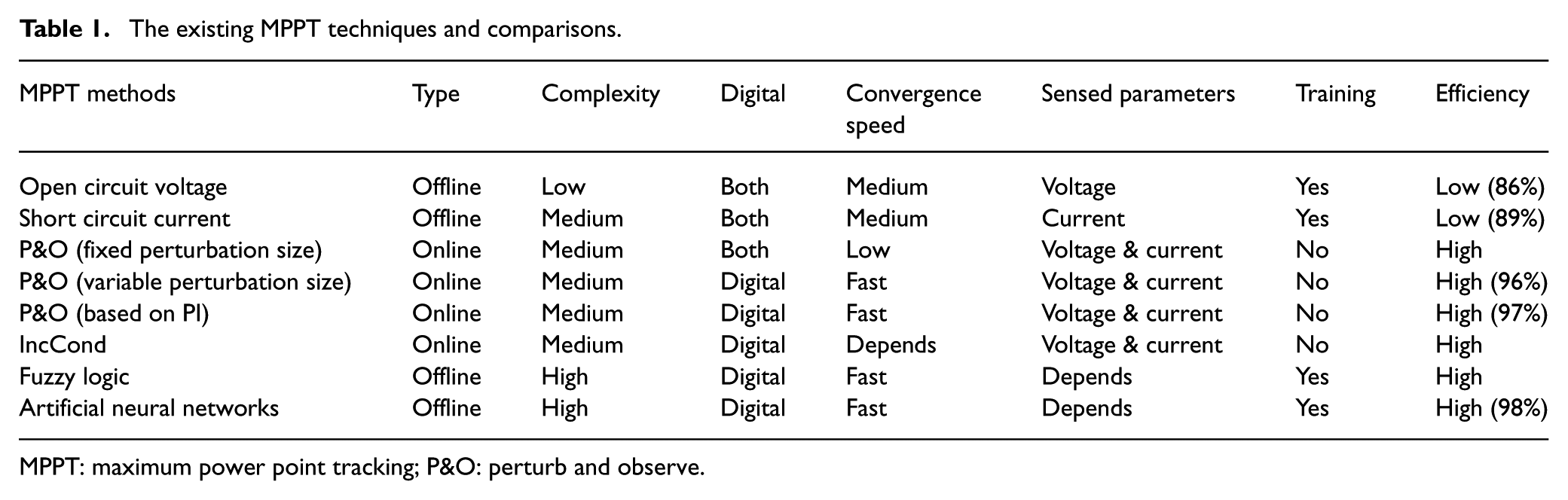
MPPT: maximum power point tracking; P&O: perturb and observe.

This indicates that the constant voltage method cannot realize MPPT in the true sense. The PV array combination method adjusts the number of arrays access based on load, so as to make PV arrays operate at MPPs. However, as the load changes quickly and with great uncertainty, this method has very poor real-time performance and fails to apply at practical situations. Some scholars propose solar tracking systems to improve the efficiency of PV panels by following the sun through the sky.

Although this method is simple in a mathematical model, it has certain problems in implementation. (1) PV arrays should be disconnected or they will short circuit when measuring the open circuit voltage $U_{oc}$ and short circuit current $I_{sc}$ , which results in unnecessary maintenance and increases some additional circuit components. (2) Indirect MPPT control method that only makes PPGS operate around MPPs, it is not a precise method for power tracking. (3) The mechanical tracking method increases construction investment costs, and targeted adjustment is required to track latitude angles.

As indirect power tracking leads to relatively large errors, research in this field has gradually transferred to direct sampling, which has no need to detect environmental factors directly, but detects the output voltage U and current I of PV arrays at the output end and calculates the power for MPPT through the U and I of PV arrays. This control method is applied widely at present. The operating principle of P&O (Brunton et al., 2010; Calais and Hinz, 1998; Nafeh et al., 2003) is to let PV arrays operate under a set voltage, increase or decrease the command value of the inverter output current, and then calculate the output power of the PV arrays. If output power increases, the perturbation direction is correct and continues to increase the output voltage of the PV arrays. If the output power decreases, perturbation direction is wrong and decreases the output current. And so the cycle continues. P&O has few measurable parameters, requiring only sampling and calculation of the output voltage and the current of the module arrays. This has a simple algorithm implementation. For example, the shorter the step-size of the fixed step-size P&O, the narrower the oscillation amplitude of the PV grid-connected system near the MPP, the less the energy loss. But the more perturbation time is required to reach the MPPs and the longer the tracking time. On the contrary, tracking speed is fast when step-size is long, but it leads to large oscillation amplitude around MPP. Too long tracking time and great power fluctuation lead to low tracking efficiency. Therefore, P&O has no ability to guarantee the speed, steady accuracy and efficiency in PPGS. In other words, it can be seen that perturbation step-size and tracking accuracy are contradictory for fixed step-size P&O (Ramaprabha et al., 2012). Some scholars have introduced variable step-sized P&O (Lalili et al., 2011; Zhang et al., 2011), which improves tracking efficiency but still cannot be applied directly in a multiple extreme point situation.

Another representative method is the IncCond method. The basics of this method is to adjust the reference command signal through detection of instantaneous conductance changes. If $\frac{d P_{PV}}{d U_{PV}} = 0$ , it indicates that the output power point of the PV arrays has reached the LMPP, the control signal command has no need to change more. This tracking method eliminates the PV array’s power oscillation at the GMPP. If the external environmental aspects change, the formula $\frac{d P_{PV}}{d U_{PV}} \neq 0$ , and then the algorithm needs to start a new tracking process for MPP. This method is also required for the output voltage U and current I detections of the PV arrays. The performance is accurate, efficient and suitable for rapid environmental change. However, this method is demanding for high accuracy of sensors, which will increase the controller’s cost. Furthermore, as computer technology and artificial intelligence continue to apply in the field of power electronics some intelligent control methods, such as fuzzy logic controller (FLC) (Chaouachi et al., 2010; Chiu, 2011; Dounis et al., 2014; Gounden et al., 2009; Hu et al., 2012; Muruganandam and Madheswaran, 2013; Ramaprabha et al., 2012; Subiyanto et al., 2012), arti_cial neural networks (ANN) (Chaouachi et al., 2010; Hiyama and Kitabayashi, 1997; Punitha et al., 2013; Singh et al., 2014b; Subiyanto et al., 2012).

FLC can solve the problem of non-linear characteristics of PV cells, but needs guaranteed suitable controller training and a lot of rules. This is obviously not practical in different applications (Kim et al., 2014; Reisi et al., 2013). ANN (Hiyama and Kitabayashi, 1997) requires an open circuit voltage $U_{oc}$ as the only input; the DC voltage $U_{dc}$ can be compared in order to determine the location of the MPP. The advantage of this method is that it improves tracking efficiency; the disadvantage is that it requires a lot of calculation. Compared with the above mentioned methods, this algorithm is relatively time consuming. For the current-to-voltage (I–V) curve of PV arrays, when the current DC-side voltage is higher than the MPP, MPPT needs to cut the output power down so as to move the current power point on the I–V curve. If the current DC-side voltage is lower than MPP, MPPT needs to improve the output power. This process of perturbation is to regulate the output power command to disturb the power point move around the MPP. It can be applied directly in a two-stage inverter. However, without a DC/DC circuit, the performance of P&O is not well applied in single-stage inverter, which negatively affects stability and efficiency. For instance, if environmental factors change sharply, the total power of PV arrays cannot support the hysteretic relatively large power command and is vulnerable to DC-side voltage collapse (see Figure 1). The voltage of PV arrays collapses down from 596 V to 488 V in 60 ms. Such a short time for regulation increases the difficulty of MPPT controller, and also makes the operation of the inverter unstable.

Figure 1.

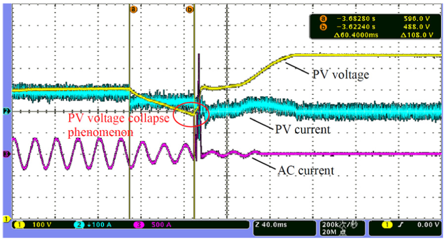
DC-side voltage collapse phenomenon.

The above mentioned methods focus on efficiency, tracking speed, LMPP optimization, and responsible solutions. However, there is little research on DC bus voltage $U_{dc}$ crashes and MPPT stability in the single-stage PV grid system. The main reflection is that the actual output power of PV modules is insufficient to make a backend inverter maintain its bus operating voltage when irradiance is weakened suddenly. Moreover, the regulation of current will further intensify the drop of the bus voltage because of the slow perturbation frequency, so the power point will move quickly towards the operating point of the open circuit current $I_{oc}$ , which is the collapse process of DC bus voltage $U_{dc}$ (Brunton et al., 2010).

Once the DC bus voltage $U_{dc}$ collapses, inverter rectification and energy back filling will occur frequently. These situations are not allowed in practical applications. When multiple MPP occurs caused by partial shadow, P&O cannot find the GMPP precisely, and then fails to track the new MPP (Jiang et al., 2014). Barrade et al. (2012) propose an improved P&O method based on tracking efficiency, speed and complexity, and discuss the distribution of MPPs under various shadow conditions. Liu et al. (2014) apply a similar method, in which the determination of GMPP is located in various DC bus segments, and then P&O is used to perturb the GMPP. This method has shortcomings such as slow tracking speed and oscillations around MPP, especially in rapidly changing environments. This makes it more difficult to configure a suitable step-size perturbation. If we apply a big perturbation step-size, the maximum power point is reached quickly, while the power loss caused by perturbation in the steady state also increases. If we use a ‘small’ perturbation step to reduce the power loss caused by perturbation in the steady state that will slow down the tracking speed. Moreover, this method doesn’t cover the fluctuation of PV-side voltage which is important in real PPGS applications.

Contributions of this paper

As discussed, the AP&O method aims to identify GMPP from multiple MPPs on power-to-voltage (P–V) curves. When the output voltage U and current I change sharply, they tend to take a big step-size to regulate the reference voltage command. When the output voltage U and current I change smoothly, this method takes a ‘small’ step size to regulate the reference voltage command (Barrade et al., 2012; Liu et al., 2014). Based on this line of thinking, this paper introduces a reference DC-side voltage $U_{dc_ref}$ disturbance to improve the stability of the DC bus voltage $U_{dc}$ . In the first stage, the algorithm divides the PV curve into several segments ranging from standby voltage $U_{standby}$ to the open circuit voltage $U_{oc}$ so as to scan the multiple LMPPs, and then locates the GMPP. In the second stage, the paper proposes the variable step-size P&O method, uses $U_{dc}$ as a perturbation target, builds an a $U / I$ dual close loop for GMPP tracking and open circuit voltage $U_{oc}$ ripple restraining. Compared with the original P&O method, AP&O has advantages such as precise location for GMPP and quick search response. Moreover, AP&O has a stronger ability to restrain the fluctuation of PV voltage, which is valuable for real PPGS applications when reducing unnecessary shutdown or maintenance cost.

The rest of this paper is organized as follows. The section ‘The topological structure and algorithm of a single-stage inverter’ introduces the structures of a PV module and a single-stage triphase inverter, and analyzes the principle of the voltage current dual-loop algorithm. The section ‘The proposed ripple based AP&O method’ presents the flowchart of a modified P&O method and explains how it is applied to a PV system. The next section, ‘Simulation and experiment’, explores the results of the proposed approach. In the final section we present our conclusions.

The topological structure and algorithm of a single-stage inverter

The mathematical model of a PV cell

Figure 2 shows the equivalent circuit of a PV cell. It includes the current source $I_{ph}$ , a diode D, equivalent resistance $R_{L}$ and parallel equivalent resistance $R_{sh}$ . In this model, the photocurrent $I_{L}$ does not change the operating state of the PV cells when irradiance is constant, and thus can be seen as a constant current source in the equivalent circuit (Barrade et al., 2012; Hartmann et al., 2013).

Figure 2.

Equivalent circuit of a PV cell.

The influence of environmental factors (i.e. irradiance, temperature, partial shadow) on the output characteristics of a PV cell shows nonlinear characteristics, and its mathematical model shows as

I = I_{ph} {\exp [\frac{q (U + R_{S} L)}{n k T}] - 1} - \frac{U + R_{S} L}{R_{sh}}

(1)

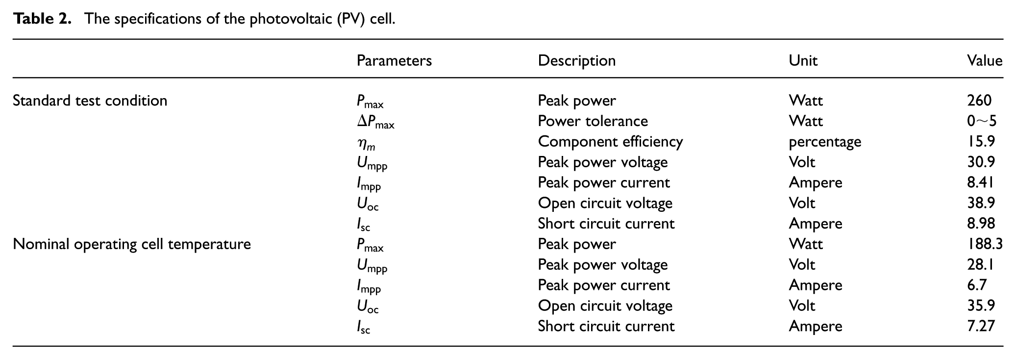
Table 2 shows the characteristic parameters of a PV cell. The conditions include a standard test condition (STC)¹ and nominal operating cell temperature (NOCT)² The P–V and I–V curves under different irradiance show in Figure 3. The curves show the following features: (1). When the temperature of the batteries doesn’t change, the greater the irradiance, the greater the $I_{sc}$ of the PV cells and the smaller the relative voltage of the constant current interval. (2). In the high voltage region, the solar cell has low internal resistance and can be viewed as a series of different levels of voltage sources. However, in the lower voltage region, the solar cell has high resistance and can be viewed as a series of different levels of current source. (3). Under any conditions, there is a PV cell maximum power point which varies along with irradiance and temperature changes. In order to fully play out the conversion capability of the PPGS, real-time tracking of the operating point of the PV cells is need to obtain maximum power output.

Table 2.

The specifications of the photovoltaic (PV) cell.

	Parameters	Description	Unit	Value
Standard test condition	$P_{max}$	Peak power	Watt	260
	$Δ P_{max}$	Power tolerance	Watt	$0 ~ 5$
	$η_{m}$	Component efficiency	percentage	15.9
	$U_{mpp}$	Peak power voltage	Volt	30.9
	$I_{mpp}$	Peak power current	Ampere	8.41
	$U_{oc}$	Open circuit voltage	Volt	38.9
	$I_{sc}$	Short circuit current	Ampere	8.98
Nominal operating cell temperature	$P_{max}$	Peak power	Watt	188.3
	$U_{mpp}$	Peak power voltage	Volt	28.1
	$I_{mpp}$	Peak power current	Ampere	6.7
	$U_{oc}$	Open circuit voltage	Volt	35.9
	$I_{sc}$	Short circuit current	Ampere	7.27

Figure 3.

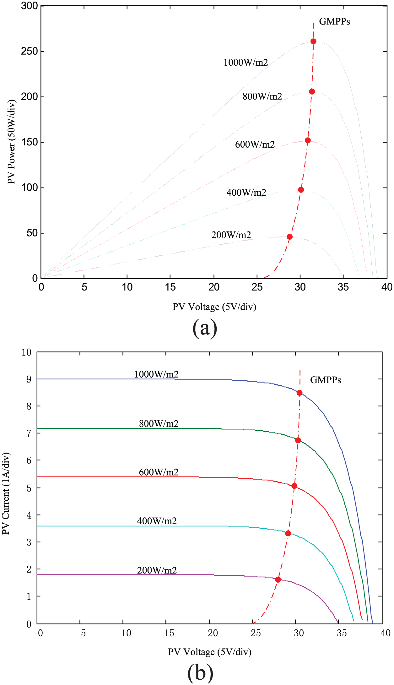
P–V and I–V curves of a solar cell. (a) P–V characteristic curves. (b) I–V characteristic curves.

Figure 3 shows the P–V characteristic curves and I–V characteristic curves under uniform conditions of irradiance. There is only one MPP on the P–V curve. But when the partly-PV module arrays are covered in shadow, multiple MPPs appear on the P–V curve. This paper illustrates the P–V curves under different conditions when a PV module is in shadow; Figure 4 shows corresponding P–V waveforms under three different non-uniform irradiance conditions. The PV arrays consist of three battery modules in series connection and the number representation in the figures shows irradiance: for example, 200 indicates that the current irradiance is 200 W/m ². From Figure 4, we arrive at the following conclusions: (1). For a single P–V curve, there are multiple MPPs in partial shadow. (2). With the array in series connection, if there are M types of irradiance, then the P–V curve presents M peak values. (3). 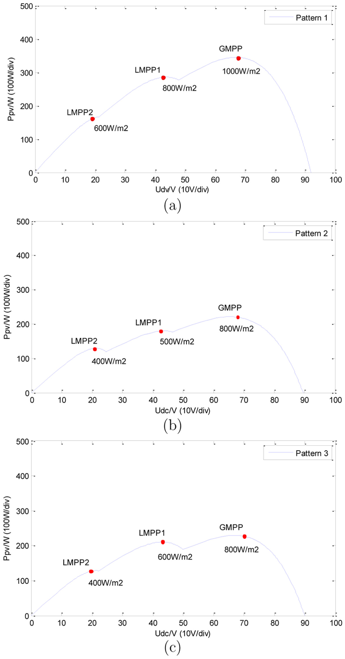Among these LMPPs, the GMPP can be effectively utilized in the range $0.5 U_{oc} ~ 0.9 U_{oc}$ . (For a single-stage PV inverter, because of the lack of a DC/DC circuit, in order to realize power conversion, DC-side voltage under $0.5 U_{oc}$ can be considered invalid; LMPPs in this segment are also ignored in real application.)

Figure 4.

PV characteristic curves of shading patterns. (a) Pattern 1. (b) Pattern 2. (c) Pattern 3.

The mathematical model of a triphase single-stage grid-connected inverter

A single-stage grid-connected PPGS commonly consists of PV arrays, a convergence device, an inverter, low-voltage switching gear and isolation boost equipment (Fadili et al., 2014; Singh et al., 2014a). Figure 5 shows the topological structure of a triphase non-midline single-stage PV grid-connected inverter, and mainly uses DC capacitors, IGBT triphase bridges, LCL filters, etc. State variables include inductive current $i_{1 a}$ , $i_{1 b}$ , $i_{1 c}$ of $L_{1}$ , voltage $u_{ca}$ , $u_{cb}$ , $u_{cc}$ of capacitor $C_{2}$ , and current $i_{2 a}$ , $i_{2 b}$ , $i_{2 c}$ on a grid-connected inductor $L_{2}$ , and the state equation is

C_{1} \frac{d u_{dc}}{dt} = i_{P V} - \sum_{k} i_{1 k} s_{k}

(2)

L_{1} \frac{d i_{1 k}}{dt} + R_{1} i_{1 k} = u_{bm} - u_{ck}

(3)

u_{mn} = u_{on} = \frac{u_{dc}}{3} \sum_{k} s_{k}

(4)

u_{kn} = u_{dc} s_{k}

(5)

i_{2 k} = i_{1 k} - i_{ck} = i_{1 k} - C_{2} \frac{d u_{ck}}{dt}

(6)

u_{ck} = u_{sk} + L_{2} \frac{d i_{2 k}}{dt} + R_{2} i_{2 k}

(7)

\sum_{k} u_{ko} = \sum_{k} u_{ck} = \sum_{k} i_{1 k} = \sum_{k} i_{ck} = \sum_{k} i_{2 o} = 0

(8)

Figure 5.

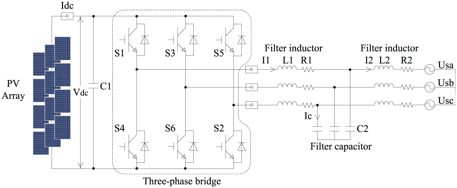
The topological structure of a triphase single-stage grid-connected inverter

Through a Clark conversion, a LCL filter state-space equation under an $α β$ static coordinate system can be obtained

{\begin{matrix} \frac{d i_{1 m}}{dt} = - \frac{R_{1}}{L_{1}} i_{1 m} - \frac{1}{L_{1}} u_{cm} + \frac{1}{L_{1}} u_{m} \\ \frac{d i_{2 m}}{dt} = \frac{1}{L_{2}} u_{cm} - \frac{1}{L_{2}} u_{sm} \\ \frac{d i_{cm}}{dt} = \frac{1}{C_{2}} i_{1 m} - \frac{1}{C_{2}} i_{2 m} \end{matrix}

(9)

A Park conversion yields a state equation under a two-line synchronous rotating coordinate system

{\begin{matrix} \frac{d i_{1 d}}{dt} = - \frac{R_{1}}{L_{1}} i_{1 d} + w i_{1 q} - \frac{1}{L_{1}} u_{cd} + \frac{1}{L_{1}} u_{d} \\ \frac{d i_{1 q}}{dt} = - \frac{R_{1}}{L_{1}} i_{1 q} - w i_{1 d} - \frac{1}{L_{1}} u_{cq} + \frac{1}{L_{1}} u_{q} \end{matrix}

(10)

{\begin{matrix} \frac{d i_{2 d}}{dt} = - \frac{R_{2}}{L_{2}} i_{2 d} + ω i_{2 q} - \frac{1}{L_{2}} u_{cd} - \frac{1}{L_{2}} u_{sd} \\ \frac{d i_{2 q}}{dt} = - \frac{R_{2}}{L_{2}} i_{2 q} - ω i_{2 d} - \frac{1}{L_{2}} u_{cq} + \frac{1}{L_{2}} u_{sq} \end{matrix}

(11)

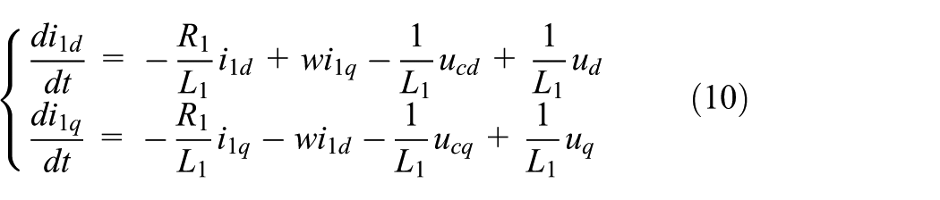
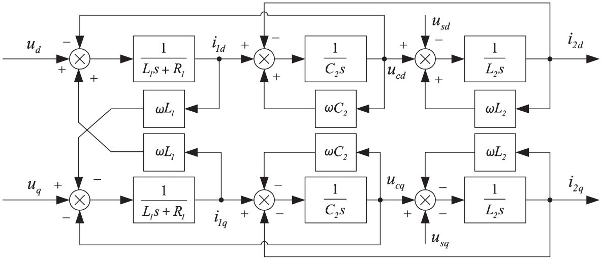
Figure 6 shows the mathematical model of an inverter under dq synchronous rotating coordinates. A mutual coupling term is introduced to the dq axis component; the current on the dq axis is not only influenced by $u_{d}$ and $u_{q}$ , but also affected by the coupling voltages $ω L_{1} i_{1 q}$ , $ω L_{2} i_{2 q}$ , $- ω L_{1} i_{1 d}$ , $- ω L_{2} i_{2 d}$ , the coupling current $ω C_{2} u_{cq}$ , $- ω C_{2} u_{cd}$ and the power grid voltage $u_{sd}$ , $u_{sq}$ . Thus, the dq axis under current closed-loop control shall be of decoupling control.

Figure 6.

The mathematical model of an inverter under dq synchronous rotating coordinates.

Figure 7 shows the control structure of an inverter, which takes dual-loop control of the bus voltage outer loop and current inner loop. The major role of the voltage loop is MPPT and active power control, and the main control method is the combination of low-frequency power perturbation algorithms with high-frequency bus voltage regulation. Power perturbation uses a fixed and variable step-size regulation mode, while bus voltage regulation is achieved by a voltage PI regulator.

Figure 7.

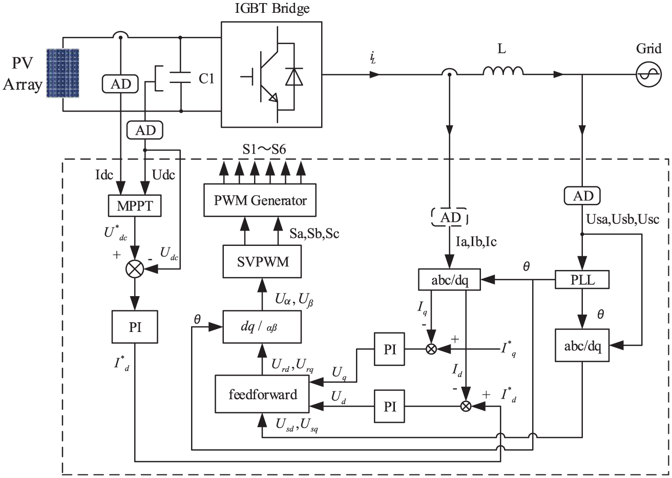
The control structure of a triphase single-stage PV grid-connected inverter.

The function of the current loop is to regulate the power, the active current and the reactive current. In order to enhance the adaptability of the inverter to the power grid, the grid’s voltage forward feed is increased in the current loop. As shown in Figure 8, without a voltage forward feed at the capacitor, the open-loop transfer function of the system is

G (s) = \frac{(K_{p} s + K_{i}) * K_{pwm} * (R_{d} Cs + 1)}{s * [L_{1} L_{2} C s^{3} + R_{d} (L_{1} + L_{2}) C s^{2} + (L_{1} + L_{2}) s]}

(12)

Figure 8.

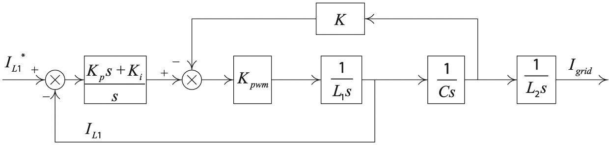
The control structure of a LCL filter.

The proposed ripple-based AP&O method

The principle of the original fixed or a variable step-size P&O method is to impose fixed or variable step-size current command signals for perturbation of power output in PV arrays. The controller calculates output power error $Δ P$ of the PV arrays, according to sampling values of DC voltage and current, and conducts $Δ P / Δ U_{dc}$ for $Δ P$ and $Δ U_{dc}$ . If the output power of the perturbed PV cells increases, that indicates that earlier perturbations can increase output power and then continue to perturb at the output voltage of the PV arrays in the same direction. On the other hand, if the output power of the PV arrays decreases after perturbation, this indicates that such perturbation is not conducive to increasing output, so the perturbation needs to be conducted in the opposite direction next time (Ji et al., 2011). This article proposes a novel two-stage P&O method. In the first stage, the PV characteristic curve is divided into several segments. Then the controller sweeps the curve and discovers some LMPPs (as shown in Figure 9), and determines the GMPP among these LMPPs. The second stage uses a variable and fixed step-size P&O method. Unlike Liu et al. (2014), the proposed method in this paper uses the DC bus voltage as the disturbance variable along with voltage-current dual loops. The advantage of this control structure that it restrains the ripple of DC voltage effectively and improves the stability of the tracking process.

Figure 9.

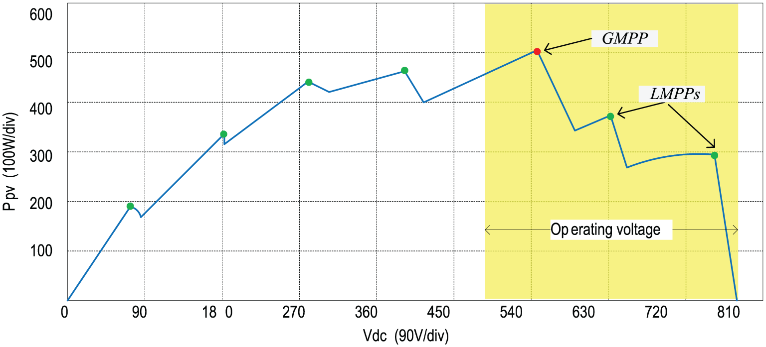
The partition schematic of PV voltage.

Figure 9 shows Liu et al. (2014)’s proposal that the voltage should be placed within the range $0.1 U_{oc}$ to $0.9 U_{oc}$ . It should be noted that, according to the normal working conditions of a single-stage inverter, the working DC voltage must be higher than the standby voltage. For this reason, this paper proposes the voltage is divided within the range from standby voltage $U_{standby}$ to open-circuit voltage $U_{oc}$ .

Figure 10 shows the proposed MPPT flowchart. The core idea of the MPPT control strategy used in this article is locating GMPP and keeping the DC voltage stable during the working state. Under this presupposition, the algorithm uses a variable step-size P&O method to improve tracking efficiency. The algorithm ensures stability and maximum power output even if the irradiance changes dramatically. The main role of the voltage loop is to maintain and perturb the DC voltage in each interval of $20 / 200$ ms. According to the accuracy of the sampling circuit board and delay of the controller, the scanning speed cannot be too fast. As Figure 10 shows, the MPPT algorithm sets different steps (STEP_N) based on the DC voltage feedback and PV power errors. The standard STEP_N is set as follows

STEP_N = M

(13)

where $M = 10 V, - 5 V, - 2 V, 0.2 V$ . At the first time of running, the controller executes the first stage algorithm, the DC voltage decreases and the DC voltage reference command shows as

{\begin{matrix} V_{dc_ref} (N) = V_{oc} - Δ V_{dc} f \\ V_{dc_ref} (N) > V_{dc_standby} \end{matrix}

(14)

where $N = 1, 2, 3$ and f is decreasing perturbation frequency of the reference voltage. N is the executed time of the controller.

Figure 10.

MPPT algorithm flow chart with variable-step length of the voltage.

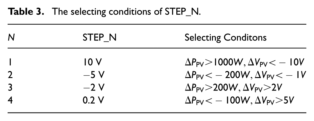
The algorithm records perturbed power values $P_{1}$ , $P_{2}$ , $P_{3}$ … $P_{K}$ in read any memory (RAM) during the decreasing reference voltage. At the same time it records the LMPPs, and then locates the GMPP $P_{max}$ and $V_{dc_\max}$ from the recorded LMPPs. On completion the first stage is ended. Due to the requirement for location speed, tracking accuracy is noncritical at the first stage. However, if the step is large, it’s more likely to ignore some LMPPs in specific voltage segments. The article sets f=5 Hz: the algorithm will perturb the DC voltage every 200 ms. When finishing the first stage of tracking, we can get basic information about GMPP such as the segment number, $Δ P_{n}$ , $Δ U_{n}$ . With these parameters, the second stage begins, the setting of STEP_N shows as follows.

When the PV power changes, depending on the error and the DC bus voltage’s error, the algorithm chooses optional STEP_N and records CNT_1, CNT_2, CNT_3, CNT_4 at each 20 ms interval. If the PV power and voltage errors meet the requirement of Table 4, then the voltage regulator executes the corresponding step-size voltage perturbation. When the power error is less than 100 W and the DC bus voltage ripple is less than 0.2 V, this indicates the maximum power point and a stable DC bus voltage. After completion of the first stage, the algorithm records the current and power values at the MPP location and takes that as the basis for the next perturbation and observation process. The controller samples DC bus voltage and current (sampling frequency is 20 kHz) and calculates the average values in accordance with every 20 ms interval. In the process of bus voltage disturbances, in order to avoid the shortcomings of traditional perturbation and observation method and fixedstep disturbance, the proposed method uses variable-step and variable frequency disturbance way, when $Δ P_{n}$ and DC bus voltage $U_{n}$ change in the large scale, then uses the a small interval (60 ms, and CNT=1). The setting of each step-size voltage disturbance is up to $Δ P_{n}$ and $U_{n}$ , as per Table 3. The advantage of the proposed method is that it tracks the GMPP rapidly, and avoids the power fluctuation under low irradiance or environmental changes. In order to avoid the unnecessary disturbance around the GMPP location, the controller uses small step-size voltage perturbations (STEP=0.2 V) at maximum intervals (CNT=4), which can reduce power spikes caused by erroneous perturbations.

Table 3.

The selecting conditions of STEP_N.

N	STEP_N	Selecting Conditons
1	10 V	$Δ P_{PV} > 1000 W, Δ V_{PV} < - 10 V$
2	$- 5$ V	$Δ P_{PV} < - 200 W, Δ V_{PV} < - 1 V$
3	$- 2$ V	$Δ P_{PV} > 200 W, Δ V_{PV} > 2 V$
4	0.2 V	$Δ P_{PV} < - 100 W, Δ V_{PV} > 5 V$

Simulation and experiment

Test rig and configuration

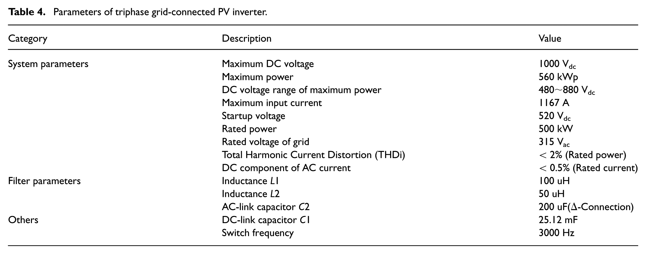
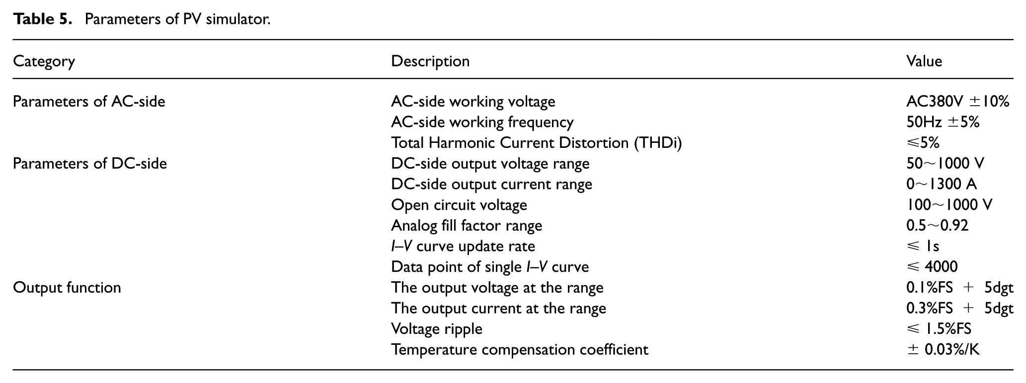
To verify the feasibility of the proposed AP&O algorithm, this paper applies Matlab/Simulink software to build a model of the whole system. It is composed of PV arrays operating at variable temperatures and irradiation. The AP&O computes the reference voltage command and the variable step size. It is worth noting that the most critical parameters for MPPT are tracking time, DC-side voltage fluctuation and conversion efficiency. They are the main reference indexes in this paper.³ In order to verify the effectiveness of the proposed method, as shown in Figure 11, experimental verification is carried out on a 500 kW single-stage prototype; the main parameters are shown in Table 4. The PV power source is a pattern of a 20-series-18-parallel (20s18p) PV panel. Meanwhile, in order to obtain repeated results, we use a 500 kW PV-simulator in this experiment; its parameters are shown in Table 5.

Figure 11.

The test schematic of the proposed method.

Table 4.

Parameters of triphase grid-connected PV inverter.

Category	Description	Value
System parameters	Maximum DC voltage	1000 V_dc
	Maximum power	560 kWp
	DC voltage range of maximum power	$480 ~ 880$ V_dc
	Maximum input current	1167 A
	Startup voltage	520 V_dc
	Rated power	500 kW
	Rated voltage of grid	315 V_ac
	Total Harmonic Current Distortion (THDi)	< 2% (Rated power)
	DC component of AC current	< 0.5% (Rated current)
Filter parameters	Inductance $L 1$	100 uH
	Inductance $L 2$	50 uH
	AC-link capacitor $C 2$	200 uF( $Δ$ -Connection)
Others	DC-link capacitor $C 1$	25.12 mF
Others	Switch frequency	3000 Hz

Table 5.

Parameters of PV simulator.

Category	Description	Value
Parameters of AC-side	AC-side working voltage	AC380V ± $10 %$
	AC-side working frequency	50Hz ± $5 %$
	Total Harmonic Current Distortion (THDi)	$\leq 5 %$
Parameters of DC-side	DC-side output voltage range	$50 ~ 1000$ V
	DC-side output current range	$0 ~ 1300$ A
	Open circuit voltage	$100 ~ 1000$ V
	Analog fill factor range	$0.5 ~ 0.92$
	I–V curve update rate	≤ 1s
	Data point of single I–V curve	≤ 4000
Output function	The output voltage at the range	0.1%FS + 5dgt
	The output current at the range	0.3%FS + 5dgt
	Voltage ripple	≤ 1.5%FS
	Temperature compensation coefficient	± 0.03%/K

Results and discussion

Figure 12 shows the DC bus voltage waveform as the inverter begins to run. It can be seen that the DC bus voltage decreases continuously during start-up. In order to shorten the scanning time, we set f=100 Hz. According to the reduction of DC-side voltage, it can be concluded that this method effectively avoids collapse of the DC bus voltage. In the next period of time, the system tracks the GMPP rapidly and stably, and finally works stably at the GMPP. Meanwhile, in order to restrain the fluctuation of PV voltage around the GMPP, the system controls output current slowly and makes corresponding changes, thus avoiding unstable work of the system or impacts on equipment due to too severe mutation of the output grid-connected current.

Figure 12.

The first stage of DC voltage scanning.

Figure 13 shows the rapid response of the MPPT algorithm to output power when the PV power mutates. The control system realizes accurate detection of step changes in illumination intensity, rapidly reduces the inverter’s output power reference value, and thus avoids collapse of the bus voltage. When the illumination reaches 40%, the simulation indicates that the system algorithm still has good stability.

Figure 13.

AC current waveform under step change of PV power. (a) AC voltage and current when PV power increases. (b) AC voltage and current when PV power decreases.

Figure 14 is the DC bus voltage waveform during inverter start-up. It can be seen that DC bus voltage decreases continuously during start-up, which effectively avoids collapse of the bus voltage. In the next period of time, the system has MPPT rapidly and stably, and finally works stably at the maximum power point. Meanwhile, in response to illumination step mutation, the system can control output current slowly and make corresponding changes, and thus avoid unstable work of system or impacts on relevant equipment due to too severe mutation of output grid-connected current.

Figure 14.

$U_{dc}$ and $i_{a}$ waveforms during start-up.

Figure 15 shows bus voltage and AC current waveforms when PV power mutates; the DC bus voltage rises when irradiance changes from weak to strong and stabilizes at a new voltage value. At this time, grid-connected current amplitude increases with the increase of commands, and finally stabilizes at a new dynamic balance point; when irradiance changes from strong to weak, DC bus voltage decreases, and stabilizes at new maximum power point voltage. The grid-connected current decreases correspondingly: with changes in irradiance, grid-connected current amplitude can be adjusted correspondingly by changing the command value of the grid-connected current directly, thus reaching a new maximum power point rapidly and stabilizing. This proves that the stability of the entire grid-connected power generation system can be guaranteed by accelerating the dynamic performance of MPPT, and a high quality grid-connected current waveform and a high power factor grid connection can still be realized under DC bus voltage fluctuation caused by dramatic changes in irradiance. Experimental results show that the system can reach a new maximum power point and work stably at the GMPP rapidly without the collapse of the DC bus voltage.

Figure 15.

Waveform tracking situation under sharp increase and sudden decrease of power. (a) $U_{dc}$ and $i_{a}$ waveforms when PV power decreases. (b) $U_{dc}$ and $i_{a}$ waveforms when PV power increases.

In order to verify the GMPP identification ability of P&O and AP&O, we set the PV simulator under three types of I–V curve, as shown in Figure 16. There are two LMMPs on each I–V curve, so the MPPT controller should take twice as much perturbation for tracking GMPP. Regarding the configuration of the P&O method, we set the variable step size as ±5 V and the fixed step size as ±2 V. From Figure 17(a), the P&O besed MPPT method takes three times as much regulation as the DC-side voltage, and during startup of the inverter, there are many perturbations of the DC-side voltage, which causes the PV voltage to fluctuate. Figure 17(b), shows that the AP&O method needs to be regulated twice for the DC-side voltage. The variable and fixed step-size are illustrated in Equation 13 and Table 3. Compare with the performance of P&O, the waveform of PV voltage does not show the fluctuations during startup and just has two regulations for voltage reduction. Regarding timing from initiation to successful location, P&O takes almost 32 seconds and the AP&O takes 24 seconds. According to tracking accuracies not listed in this paper, the total tracking efficiencies of P&O and AP&O are 96.6% and 98.3% respectively. The total distortion rate of DC-side voltage are 8.33% and 3.5% respectively. The lower total distortion rate of DC-side voltage illustrates that AP&O has stronger ability to restrain the DC-side voltage fluctuation, which is important for stable operation in PPGS.

Figure 16.

Three types of I–V curve given by the PV simulator.

Figure 17.

$U_{dc}$ and $i_{a}$ waveforms. (a) $U_{dc}$ and $i_{a}$ waveforms based on P&O method. (b) $U_{dc}$ and $i_{a}$ waveforms based on AP&O method.

Conclusions

This paper proposes a novel two-stage algorithm using the AP&O method. It applies a voltage ripple-based loop to calculate the fixed and variable step-size of perturbation in a single-stage PV grid-connected inverter. In the first stage, the PV curve is divided into multiple segments in a range from standby voltage $U_{standby}$ to open-circuit voltage $U_{oc}$ . The GMPP location can be computed by scanning the series of LMPPs. In the second stage, the paper proposes the variable step-size P&O method, uses the $U_{dc}$ as a perturbation target, builds a $U / I$ dual closed loop for GMPP tracking and open circuit voltage $U_{oc}$ ripple restraining. After simulating all possible shading patterns on the 20s18p PV panel in PPGS, the results show that the average tracking accuracy meets the requirement of China’s test standard NB/T 32004-2013. Experiments are carried out with three different shadow patterns. A comparison shows that the proposed method can obtain GMPP of different shading patterns and the tracking accuracies are all higher than the original P&O method. These results confirm that the proposed method could be successfully implemented in PPGS. AP&O inherits P&O’s advantages, such as precise location for GMPP and quick responses for new seeking requirements. This method has advantages on restraining the fluctuation of PV voltage and improves the tracking accuracy of voltage and the current loop. Compared to conventional single-stage algorithms, this method improves tracking efficiency, maintains system stability under rapidly changing environmental conditions and effectively avoids the bus voltage collapse phenomenon. The experimental results show that the precision and control stability are valid in real applications.

Footnotes

Funding

The author(s) disclosed receipt of the following financial support for the research, authorship, and/or publication of this article: The authors would like to thank the University of Macau for its funding support under grant number MYRG2015-00077-FST.

Notes

References

Barrade

Delalay

Rufer

(2012) Direct connection of supercapacitors to photovoltaic panels with on-off maximum power point tracking. IEEE Transactions on Sustainable Energy 3(2): 283–294.

Brunton

Rowley

Kulkarni

et al . (2010) Maximum power point tracking for photovoltaic optimization using ripple-based extremum seeking control. IEEE Transactions on Power Electronics 25(10): 2531–2540.

Calais

Hinz

(1998) A ripple-based maximum power point tracking algorithm for a single-phase, grid-connected photovoltaic system. Solar Energy 63(5): 277–282.

Chaouachi

Kamel

Nagasaka

(2010) A novel multi-model neuro-fuzzy-based mppt for three-phase grid-connected photovoltaic system. Solar Energy 84(12): 2219–2229.

Chiu

(2011) T-s fuzzy maximum power point tracking control of solar power generation systems. IEEE Transactions on Energy Conversion 25(4): 1123–1132.

Dounis

Kofinas

Alafodimos

et al . (2014) Adaptive fuzzy gain scheduling PID controller for maximum power point tracking of photovoltaic system. Renewable Energy 60(4): 202–214.

El-Nafeh

Fahmy

El-Zahab

EMA

(2003) Evaluation of a proper controller performance for maximum-power point tracking of a stand-alone PV system. Solar Energy Materials & Solar Cells 75(3): 723–728.

Fadili

A El

Giri

Magri

A El

(2014) Reference voltage optimizer for maximum power point tracking in triphase grid-connected photovoltaic systems. International Journal of Electrical Power & Energy Systems 60(11): 293–301.

Fusco

Russo

(2013) Design of decentralized robust controller for voltage regulation and stabilization of multimachine power systems. International Journal of Control Automation & Systems 11(2): 277–285.

10.

Ghoddami

Yazdani

(2011) A single-stage three-phase photovoltaic system with enhanced maximum power point tracking capability and increased power rating. IEEE Transactions on Power Delivery 26(2): 1017–1029.

11.

Gounden

Peter

Nallandula

et al . (2009) Fuzzy logic controller with mppt using line-commutated inverter for three-phase grid-connected photovoltaic systems. Renewable Energy 34(3): 909–915.

12.

Hartmann

Vitorino

Correa

MBR

et al . (2013) Combining model-based and heuristic techniques for fast tracking the maximum-power point of photovoltaic systems. IEEE Transactions on Power Electronics 28(6): 2875–2885.

13.

Hiyama

Kitabayashi

(1997) Neural network based estimation of maximum power generation from module using environmental information. IEEE Transactions on Energy Conversion 12(3): 241–247.

14.

Yang

Zhu

et al . (2012) Constrained markov control model and online stochastic optimization algorithm for power conservation in multimedia server cluster systems. International Journal of Control Automation & Systems 10(6): 1215–1224.

15.

Ishaque

Salam

(2013) A review of maximum power point tracking techniques of PV system for uniform insolation and partial shading condition. Renewable & Sustainable Energy Reviews 19(1): 475–488.

16.

Ishaque

Salam

Lauss

(2014) The performance of perturb and observe and incremental conductance maximum power point tracking method under dynamic weather conditions. Applied Energy 119(12): 228–236.

17.

Jung

Kim

et al . (2011) A real maximum power point tracking method for mismatching compensation in PV array under partially shaded conditions. IEEE Transactions on Power Electronics 26(4): 1001–1009.

18.

Jiang

Han

Wang

et al . (2014) Maximum power point tracking scheme for PV systems operating under partially shaded conditions. Control Engineering of China 55(4): 1689–1698.

19.

Kim

Son

Lee

(2014) Use of model predictive controller in dual-loop control of three-phase pwm ac/dc converter. International Journal of Control Automation & Systems 12(2): 340–348.

20.

Lalili

Mellit

Lourci

et al . (2011) Input output feedback linearization control and variable step size MPPT algorithm of a grid-connected photovoltaic inverter. Renewable Energy 36(12): 3282–3291.

21.

Liu

Chen

Huang

(2014) Global maximum power point tracking algorithm for PV systems operating under partially shaded conditions using the segmentation search method. Solar Energy 103(6): 350–363.

22.

Muruganandam

Madheswaran

(2013) Stability analysis and implementation of chopper fed DC series motor with hybrid PID-ANN controller. International Journal of Control Automation & Systems 11(5): 966–975.

23.

Patel

Agarwal

(2008) Matlab-based modeling to study the effects of partial shading on Pv array characteristics. IEEE Transactions on Energy Conversion 23(1): 302–310.

24.

Punitha

Devaraj

Sakthivel

(2013) Artificial neural network based modified incremental conductance algorithm for maximum power point tracking in photovoltaic system under partial shading conditions. Energy 62(6): 330–340.

25.

Ramaprabha

Balaji

Mathur

(2012) Maximum power point tracking of partially shaded solar PV system using modified fibonacci search method with fuzzy controller. International Journal of Electrical Power & Energy Systems 43(1): 754–765.

26.

Reisi

Moradi

Jamasb

(2013) Classification and comparison of maximum power point tracking techniques for photovoltaic system: A review. Renewable & Sustainable Energy Reviews 19(1): 433–443.

27.

Singh

Jain

Goel

(2014a) ILST control algorithm of single-stage dual purpose grid connected solar PV system. IEEE Transactions on Power Electronics 29(10): 5347–5357.

28.

Singh

Shahani

Verma

(2014b) Neural network controlled grid interfaced solar photovoltaic power generation. IET Power Electronics 7(3): 614–626.

29.

Subiyanto

Mohamed

Hannan

(2012) Intelligent maximum power point tracking for PV system using hopfield neural network optimized fuzzy logic controller. Energy & Buildings 51(8): 29–38.

30.

Yang

Hsieh

Feng

et al . (2012) Highly efficient analog maximum power point tracking (AMPPT) in a photovoltaic system. IEEE Transactions on Circuits & Systems I Regular Papers 59(7): 1546–1556.

31.

Zhang

Hurley

WoLfle

(2011) A new approach to achieve maximum power point tracking for PV system with a variable inductor. IEEE Transactions on Power Electronics 26(4): 948–952.