






Abstract
The paper deals with the recursive identification of time-varying non-linear dynamic systems using three-block cascade models with non-linear static, linear dynamic and non-linear dynamic blocks. These models are appropriate for systems with both actuator and sensor non-linearities. Multiple application of a decomposition technique provides special expressions for the corresponding non-linear model description that are linear in parameters. A modified recursive least-squares-based algorithm is used for estimation of the time-varying input polynomial and output backlash parameters. Simulation studies show the feasibility of proposed approach to estimate the model parameters and track their changes.
Introduction
Non-linear cascade models are a popular type of block-oriented models, i.e. when linear dynamic blocks are in a tandem connection with static non-linear blocks. These models are used in mathematical modelling of non-linear dynamic systems not only for their relative simplicity but also for their ability to approximate closely more general non-linear systems, which are not necessarily of this form. The so-called Hammerstein model consists of a static non-linear block followed by a linear dynamic block and is supposed to represent actuator non-linearities. There are many identification methods for different types of non-linearities and corresponding models. For example, many identification methods have been presented for the Hammerstein systems using different iterative algorithms (e.g. Chen H et al., 2014; Deng and Ding, 2014; Shen and Ding, 2014; Vörös, 1999; Wang and Ding, 2016c) or recursive algorithms (e.g. Ding et al., 2016b; Wang et al., 2013, 2014; Wang and Ding, 2016b; Zhao et al., 2013). Some approaches deal with special types of non-linearities (e.g. Giri et al., 2008; Pupeikis, 2006; Zhang and Mao, 2015) or are based on non-parametric models (e.g. Hasiewicz and Mzyk, 2004; Sliwinski et al., 2009).
The so-called Wiener model consists of a linear dynamic block followed by a static non-linear block and is supposed to represent sensor non-linearities. The identification of non-linear dynamic systems using Wiener models has been an active research area for many years and many approaches have been presented using parametric models (e.g. Bai and Reyland, 2009; Chen J et al., 2014; Ding et al., 2016a; Giri et al., 2009; Janczak, 2007; Kazlauskas and Pupeikis, 2013; Vörös, 2007; Wang and Ding, 2011; Wang and Ding, 2016a; Zhou et al., 2014) or based on non-parametric methods (e.g. Pawlak et al., 2007; Wachel and Mzyk, 2016).
If the systems to be identified contain non-linearities with memory such as backlash or hysteresis (Kalaš et al., 1985), the choice of Hammerstein or Wiener models is not appropriate, because the non-linear static blocks cannot characterize these dynamic non-linearities. Therefore, a special case of two-block models consisting of the cascade of linear dynamic and non-linear dynamic blocks has to be used for modelling and identification of non-linear dynamic systems with backlash or hysteresis. The cascade model structure consisting of a linear dynamic block followed by a non-linear dynamic block was often used for the identification of non-linear dynamic systems with output backlash (e.g. Giri et al., 2014; Vörös, 2010).
However, in the case of more complex non-linear dynamic systems with both input and output non-linearities, it is appropriate to choose a three-block cascade model with combination of non-linear static, linear dynamic and non-linear dynamic blocks (Vörös, 2015). This means, compared with the well-known structure of Hammerstein–Wiener model, that the output block contains dynamic non-linearities, e.g. backlash or hysteresis. Actually, this form of three-block cascade model can significantly extend the applicability for more precise modelling and identification of real systems with both actuator and sensor non-linearities.
In this paper, the three-block cascade model is used to the recursive identification of time-varying non-linear dynamic systems with a static input non-linearity and an output backlash. To the author’s knowledge, no work dealing with this problem has been published until now. The previous results on the decomposition of compound operators (Vörös, 1999, 2007) are effectively applied to simplify the mathematical description of this complex system. The resulting model equation is without cross-multiplication of parameters; nevertheless, it contains more internal variables, which are generally unmeasurable. Application of a modified least-squares-based recursive algorithm enables estimation of all the model parameters and internal variables on the basis of measured input/output data. Simulation studies of cascade systems identification with time-varying input polynomial and time-varying output backlash characteristics are included to demonstrate the feasibility of the proposed approach to estimate the model parameters and track their changes.
The paper is organized as follows. The next section gives the description of three-block cascade model with polynomial non-linearity and output backlash. A recursive parameter estimation algorithm is derived and simulation studies for the proposed algorithm are provided. Finally, concluding remarks are given.
Three-block cascade model
Let the three-block cascade model be given by the cascade connection of a non-linear static block followed by a linear dynamic block, which is followed by a non-linear dynamic block according to Figure 1.

Three-block cascade model with output backlash.
The characteristic of non-linear static block with input u(t) and output v(t), for the discrete time t=1, 2, …, can be approximated by the polynomial
and assume that the characteristic may be time-varying, i.e. the parameters gk can change in time. The linear dynamic block (LD) can be described by the difference equation
where v(t) and x(t) are the inputs and outputs of the LD, respectively. It is assumed that the linear dynamic system is stable.
Let the non-linear output dynamic block be a backlash with inputs x(t) and outputs y(t) shown in Figure 2. The backlash is a dynamic non-linearity and can be described by the following first-order non-linear difference equation (Vörös, 2010)
where f1(t) and f2(t) are auxiliary internal variables defined as:
and h(.) is a switching function defined as follows
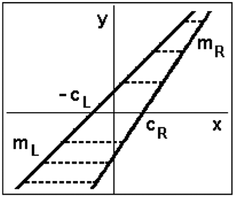
Output backlash.
We assume that the backlash may be time-varying, i.e. the parameters mL, cL, mR and cR can change in time.
The mathematical description of this cascade system resulting from direct substitutions of the corresponding variables from (1) into (2) and then into (3) is strongly non-linear, both in the variables and in the parameters, and hence not very suitable for the parameter estimation. To find a simpler form of this description, the so-called key-term separation principle with half-substitutions will be applied (Vörös, 1999, 2007). Because of the cascade connection of three blocks, the parameterization of three-block cascade models is not unique; many combinations of parameters can be found. Therefore, in at least two blocks, one parameter has to be fixed. Choosing mL=1, we rewrite (3) as follows:
and half-substitute (2) into (7), i.e. only for x(t) in the first term
assigning
Then we can choose a1=1 and half-substitute (1) into (8), i.e. only for the term with variable v(t−1). This will lead to the three-block cascade model output equation
where e(t) is a white noise with zero mean. This equation is linear in all the cascade model block parameters, but non-linear in some variables. The model inputs u(t) and outputs y(t) are measurable, whereas the internal variables v(t), x(t), f1(t) and f2(t) are not. As has been mentioned above, the parameters of both the static and the dynamic non-linearities can change with time.
Recursive parameter estimation
The three-block cascade model equation can be written in the following concise form
where
is the vector of data,
is the vector of parameters and yc(t) is the so-called corrected output.
Assume that the constants n, p and r are known and y(t)=0, u(t)=0 and x(t)=0 for t≤0. The recursive parameter estimation for the cascade system with output hysteresis can be performed minimizing the quadratic criterion
where 0<λ≤1 is the forgetting factor. However, the variables v(t), x(t), f1(t) and f2(t) are not available and must be estimated; therefore the data vectors φ(j) in (14) will be replaced by their estimates containing the estimates of corresponding internal variables and the well-known recursive identification algorithm (Ljung and Söderström, 1983) will be supplemented with the estimation of internal variables as follows:
where µ is a large constant, the new values (estimates) of all the internal variables for the data vector in each recursion are computed by (15)–(18) and the corrected output is computed by (21) using the previous estimates of corresponding parameters. The first estimates of backlash parameters must be chosen as non-zero enabling the computation of the first estimates of internal variables f1(t), f2(t) and the value of corrected output yc(t). The initial values of the linear system parameters can be chosen to be zero.
The use of forgetting factor λ is particularly useful in order to assign less weight to errors computed in the early steps of the procedure. However, as λ decreases, noise sensitivity increases (Chidambaram, 2001). Therefore, it is appropriate to use two forgetting factors – the smaller one at the beginning to reduce the influence of erroneous internal variables estimates and later a larger one to reduce the influence of eventual noise.
Simulation studies
The following examples of simulated time-varying three-block cascade systems with polynomial input block and output backlash illustrate the feasibility of the proposed approach to estimate the model parameters and track their changes.
Example 1
The characteristic of the input static block was described by the original polynomial
(the thin/blue line in Figure 3) that was changed during the process to the new characteristic (the thick/green line in Figure 3). The corresponding values of the parameters are given in Table 1.
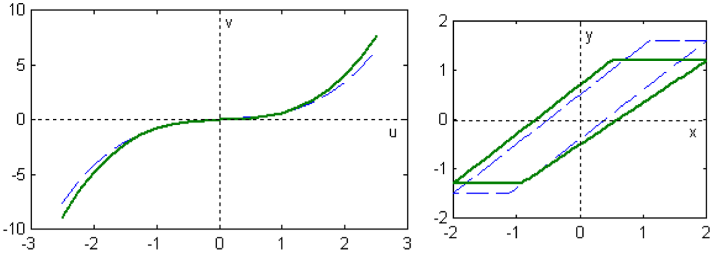
Example 1 – input non-linearity (left) and output backlash (right).
Example 1 – the parameter values.

The linear dynamic block LD was given by the difference equation
and was followed by the output backlash with parallel lines characterized by the original parameters mL=1.0, cL=0.5, mR=1.0 and cR=0.4 (the thin/blue line in Figure 3). This was changed during the process to the new backlash characteristic with parameters given in Table 1 (the thick/green line in Figure 3).
The recursive identification was performed on the basis of 4000 samples of uniformly distributed random inputs with |u(t)|<2.0 and simulated outputs. The changes of polynomial and backlash parameters occurred slowly and gradually in the time interval t∈(1500, 1900). To make the simulation more realistic, normally distributed random noise with zero mean and the signal-to-noise ratio (the square root of the ratio of output and noise variances), SNR=100, was added to the generated outputs. The algorithm was applied with initial values mR=0.5 and cL=cR=0.001 for the first estimates of internal variables, whereas the initial values of the linear system parameters were chosen to be zero. Two forgetting factors were used in this example, i.e. λ=0.92 for the first 100 samples and λ=0.995 for the rest of data.
The process of estimation of the model parameters is shown in Figure 4, where the estimates of three polynomial parameters g1(t), g2(t) and g3(t) soon attained their true values, then two parameters began to change to new values (Table 1) and finally remained unchanged, except the small deviations caused by the output noise. The estimates of linear block parameters a2(t), b1(t) and b2(t) were only slightly influenced by the changes of other parameters. The process of estimation of the backlash parameters is shown in Figure 4 (bottom), where the estimates of parameters mR(t), cL(t) and cR(t) soon attained their true values, then all parameters began to change to new values (Table 1) and finally remained unchanged, except for the small deviations caused by the output noise. It can be seen that the proposed identification algorithm is able to track the system parameters and their changes.
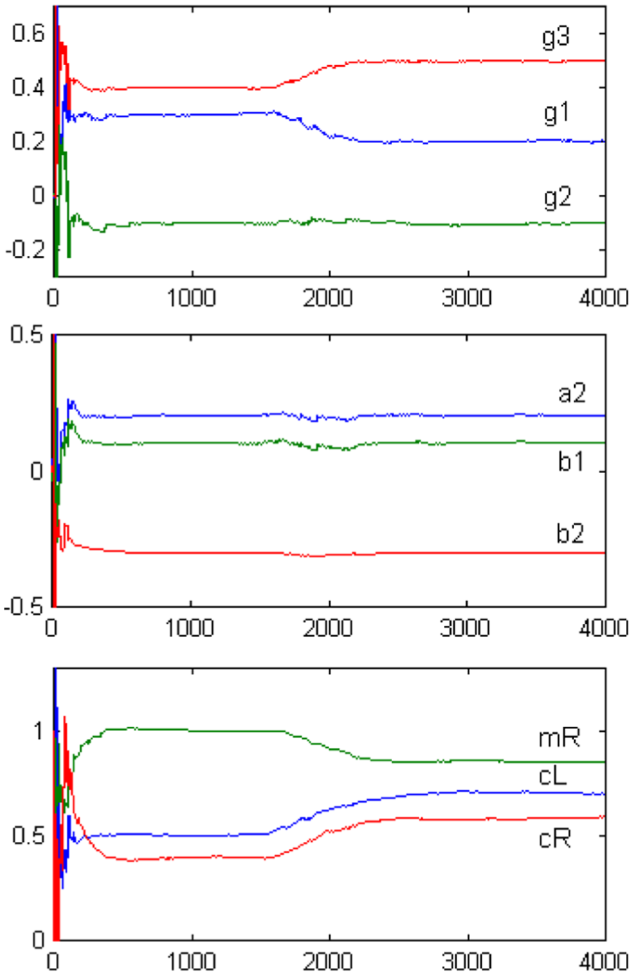
Example 1 – the process of polynomial, linear dynamic block (LD) and backlash parameters estimation.
Example 2
The characteristic of the input static block was described by the original polynomial
(the thin/blue line in Figure 5) that was changed during the process to the new characteristic (the thick/green line in Figure 5). The corresponding sets of parameters are given in Table 2. The linear dynamic system was the same as in Example 1; however, the output backlash was considered with non-parallel lines and characterized by the original parameters mL=1.0, cL=0.5, mR=1.2, cR=0.4 (the thin/blue line in Figure 5). This was changed during the process to the new backlash characteristic with parameters given in Table 2 (the thick/green line in Figure 5).
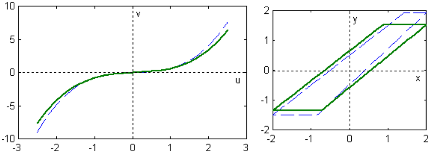
Example 2 – input non-linearity (left) and output backlash (right).
Example 2 – the parameter values.

The identification was performed under the same conditions as in Example 1. The process of estimation of the model parameters is shown in Figure 6.
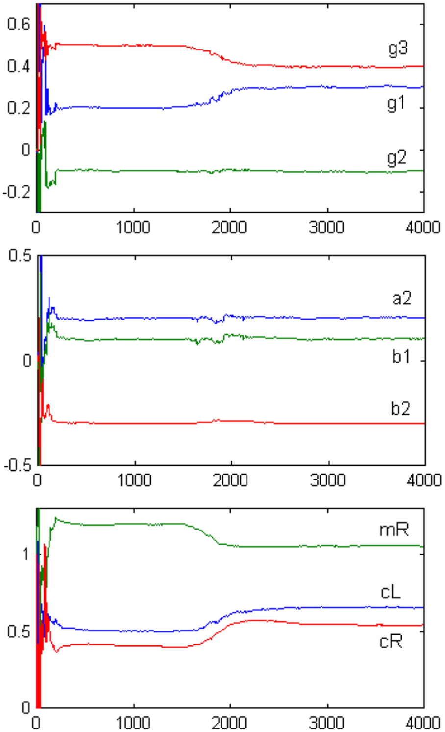
Example 2 – the process of polynomial, linear dynamic block (LD) and backlash parameters estimation.
Example 3
The characteristic of input static block was the linear function given by
(the thin/blue line in Figure 7) that was changed during the process to the non-linear function (the thick/green line in Figure 7). The corresponding values of the parameters are given in Table 3. The linear dynamic system was the same as in Example 1 and the output backlash with parallel lines was characterized by the original parameters mL=1.0, cL=0.5, mR=1.0 and cR=0.4 (the thin/blue line in Figure 7). This was changed during the process to the new backlash characteristic with parameters given in Table 3 (the thick/green line in Figure 7).
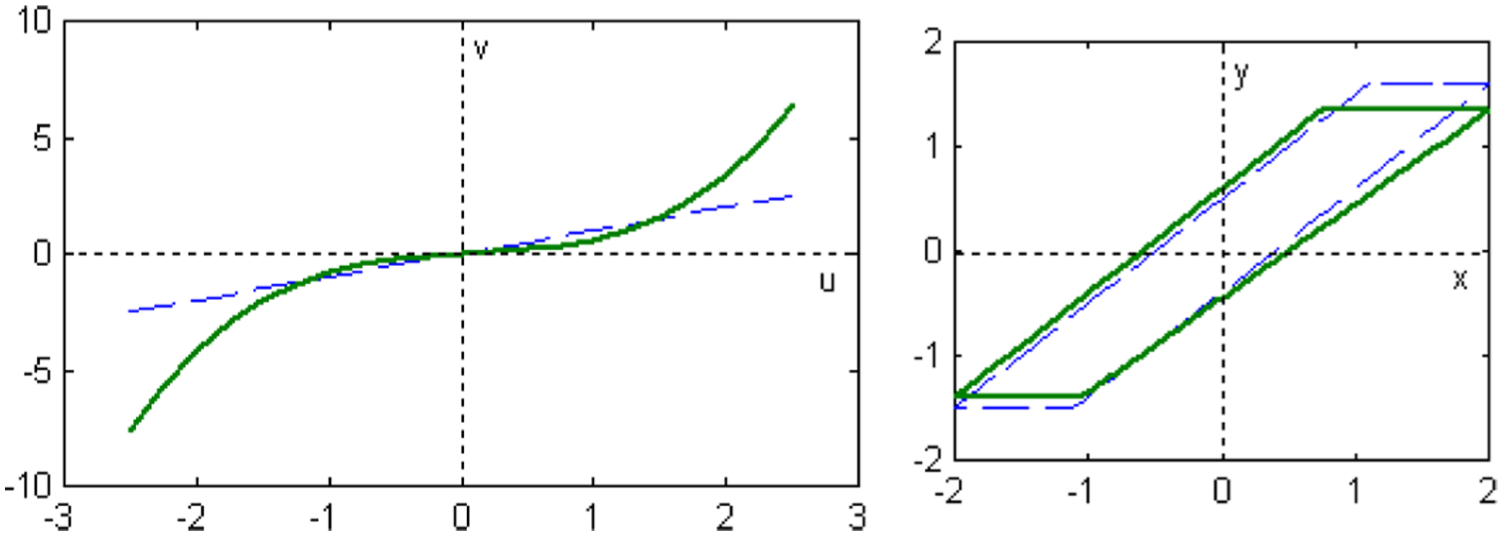
Example 3 – input non-linearity (left) and output backlash (right).
Example 3 – the parameter values.

The identification was performed under the same conditions as in Example 1. The process of estimation of the model parameters is shown in Figure 8. In this case, the linear characteristic in the input block was changed to a non-linear one and all the parameters of both non-linear blocks were changed. The proposed identification algorithm was able to track the model parameters and their changes in this extreme case of time-varying behaviour.
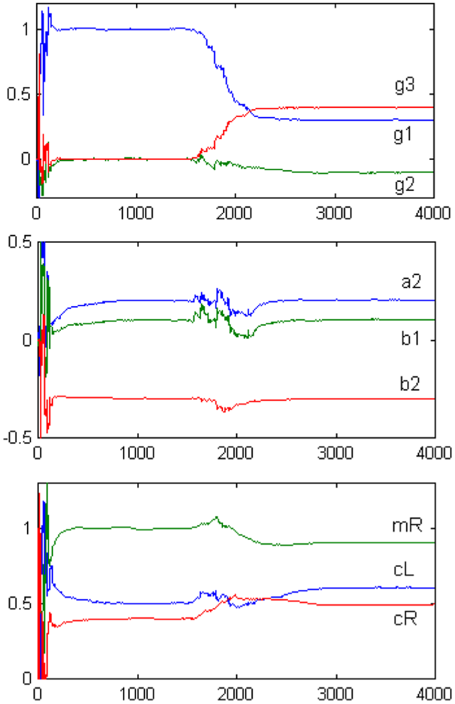
Example 3 – the process of polynomial, linear dynamic block (LD) and backlash parameters estimation.
Conclusion
The presented recursive approach to the identification of time-varying non-linear dynamic systems is based on the three-block cascade models with static input and dynamic output non-linearities. These models are appropriate for systems with both actuator and sensor non-linearities. Until now, no results have been published on the identification of systems with time-varying input and output non-linearities. The identification is based on a special form of model description resulting from more consecutive decompositions of compound mappings describing this block-oriented model. A modified recursive least-squares-based parameter estimation algorithm with estimations of internal variables has been proposed and studied on examples of simulated non-linear dynamic systems with polynomial non-linearities in the input block and with the backlash in the output block.
Finally, note that the presented identification method can be easily extended for time-varying systems with the so-called general output backlash (Reyland and Bai, 2014; Vörös, 2012) and other types of time-varying static non-linearities can be considered in the input block of three-block cascade models.
Footnotes
Acknowledgements
The author gratefully acknowledges financial support from the Slovak Scientific Grant Agency (VEGA).
Declaration of Conflicting Interests
The author declares that there is no conflict of interest.
Funding
This research received no specific grant from any funding agency in the public, commercial or not-for-profit sectors.