
Abstract
This work treats the physical one-dimensional (1D) and two-dimensional (2D) modelling of a chemical process of filtration of slurry, which is the second step of phosphoric acid manufacture. This work focuses on the different physical laws involved in the filtration stage in order to obtain a simulator of the filter. In this work, we are interested in the 1D modelling of a rotary filter using all parameters and physical phenomena established in the filtration phase. Then, a 2D model emerged from the previous model by choosing both a temporal and a spatial variable. These two parameters are quite necessary for the construction of a 2D model based on the method of Fornasini–Marchesini (FM-II) to describe the dynamics of the system.
Introduction
In recent years, membrane filtration technology, especially low pressure membrane technology, has been more widely applied in liquid aspiration fields (Pei et al., 2007).
Well known for some time, the membrane separation processes are considered advanced, efficient, and beneficial technologies to use. These methods are used to separate suspended particles. The filtration technique is recognized in porous membranes and follows the pore size. There are four levels of filtration: macrofiltration, microfiltration, ultrafiltration, and nanofiltration (Zart, 2008). Filtration processes can be classified into two categories:
discontinuous process: the press filter and the Nutshe filter are the most prevalent;
continuous process: the rotary drum filter and the pass band filter are the most prevalent.
In our case, a rotary drum filter will be described which ensures the separation between the phosphoric acid and the phosphogypsum. In the literature, few works have dealt with the filtering modelling due to its complexity and the number of parameters interfering in the filtration process. The problem is therefore to successfully model the system to be studied. So, we want to develop a model close to the real system.
The modelling filter is essentially based on Darcy’s law treated by Nicolas (2003) which applies to a homogeneous and isotropic porous middle. This middle is traversed by a flow at low speed in order to calculate the rate of phosphoric acid produced. Darcy’s law is also processed by Chassagne (2010) and a similar strategy has been discussed by Darcy (1938). Then a relationship frequently quoted was proposed by Robert and Obertin (2003) and modified by Carman (1938). The multiple physical equations that are based on the parameters such as specific resistance using the method of Wu and Zhang (2010) are exploited. As Robert and Obertin (2003) has treated the coefficient of permeability and permeability models whilst seeking to establish an expression depending on the geometry of the pore network. Finally the porosity (the main parameter) for describing a porous middle is outlined by Nicolas (2003).
In this research a pseudo-homogeneous two dimensional model was proposed to describe the dynamic behaviour of a rotary filter. The interest in two-dimensional (2D) systems goes back to the early seventies (Fornasini and Marchesini, 1978), and has gained momentum due to its extensive use. 2D systems have drawn considerable attention because of their wide range of practical applications and the significant theoretical importance. 2D system theory can be used efficiently in many fields such as multidimensional signal processing and digital filtering, multi-variable network modelling, digital picture processing, seismic data processing, thermal processes, and batch processes (Kaczorek, 2006; Liu and Wang, 2012; Renard, 1996; Tse, 1973). Therefore, considerable interest has emerged in the theoretical analysis and synthesis of 2D systems, resulting in a large number of compelling research results in the literature. For instance, investigations on 2D systems have been conducted related to the state-space model realization (Chen, 1999; Kaczorek, 2006), stability and stabilization (Chesi and Middleton, 2014; Souza and Osowsky, 2013), estimation and observers (Bisiacco, 1985a; Liang et al., 2014; Xu et al., 2012), and filtering (Gao, 2013; Wu and Wang, 2015; Zhao et al., 2014).
More recently, many other interesting contexts where 2D systems prove to be the appropriate setting have been enlightened (Bisiacco and Valcher, 2015; Xu et al., 2004). Indeed, in the one-dimensional (1D) context, there has been a long stream of research on this subject, which originated in the seventies and flourished in the eighties (Du and Xie, 2002; Kurek, 1983), but still represents a very lively topic of research. During the last thirty years, research interests in 2D system theory have been focused on most of the classical topics already investigated in the 1D setting (Bisiacco, 1985b; Fornasini and Zampieri, 1990; Kaczorek, 2002; Liang et al., 2014). More generally the most interesting point of the 2D systems is related to the fact that they depend on two invariant variables where generally one of them is time and the other is spatial. However there are many 2D systems such that neither of their variables are time or spatial (Kaczorek, 2008; Liu, 2015; Paran and Adloo, 2004; Shong Hong, 2010). Moreover, one of the fundamental issues in 2D systems theory is the realization of a given transfer function or transfer matrix by a certain kind of 2D local state space model, typically by the Roesser model or the Fornasini–Marchesini second (FM-II) model.
The rotary filter is a fairly giant industrial process that works in real time. In this context, it is impossible to stop the system to do tests, to take measures or to make variations on the control variables. So here we need a 1D model close to the real system that allows us to perform simulations and to better understand the operation of the actual process and to control it. Regarding the 2D model, it is more accurate than the 1D model because it is based on two spatial and temporal parameters.
Our contribution is mainly based on the modelling of a rotary drum filter using physical laws and with the realization problem for a given 2D Multi-Input Multi-Output (MIMO) system by FM-II model. This paper is organized as follows: Section ‘1D non-linear modelling of rotary drum filter’, describes the 1D non-linear modelling of the filter using several laws. Section ‘2D modelling based on FM-II method’ describes the 2D modelling of the rotary filter and the implementation of the FM-II method algorithms. Finally, concluding remarks are made.
1D non-linear modelling of rotary drum filter
The literature generally distinguishes between two types of approach to model filtration: macroscopic models based on the material conservation equations and a filtration rate which is determined empirically, and microscopic models describing the grain transportation process. Concerning macroscopic models, these types are not based on the physical modelling of the particle deposition mechanisms. The parameters of these models do not necessarily have a clear physical meaning but the results are usually close to the experimental results.
Developing a model first requires us to write mathematical equations that relate state variables descriptive of physical process. When compared to other procedures the filtration system of fixed cultures has the complementary particularity to include an additional model of physical filtration, which increases the difficulty of resolution and integration of system equations. For activated sludge processes like the filter, the problem of the complexity of the models make the control possibilities in practice very limited (Gomez–Quintero, 2002).
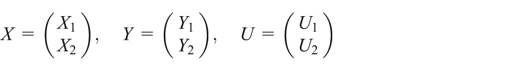
The model we’re looking for is a model for a control objective. So we will look for the physical equations that contain the state variables X and control variables U.
The rotary drum filter description
These are mainly devices for running empty including: rotary drum filters and belt filters. They have the same applications but the band filters deal thicker slurries (50% solids). Among the filters that are considered continuous we find the rotary drum filter. The rotary drum filter is constituted by two coaxial cylindrical drums, the outer drum carries a filter canvas (see Figure 1).
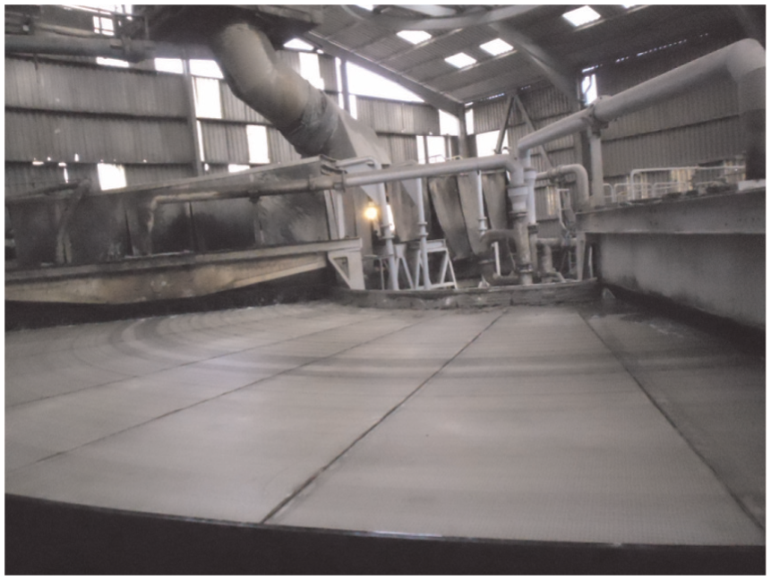
Rotary drum filter.
In recent years, membrane filtration technology, especially low pressure membrane technology, has been more widely applied in liquid aspiration fields. Based on this technology, the phosphoric acid plant acquires a huge filter from the ”AOUSTIN-UCEG” company. This filter is composed of 36 flat cells covered by 36 membranes with 36 tubes where each tube is connected to a cell, a vacuum box, and a driving motor which is responsible for the transition of the slurry by five sectors which are: the pre-sector, the strong acid sector, the acid medium sector, the weak acid sector, and the sector of wash canvases. Figure 1 shows a photo of the filter.
Formulation of the mathematical model
Calculation of the height of the cake equation ‘h’
According to the mass balance, the quantity of the slurry in the filter is equal to the difference between the quantity of slurry injected into the filter and the quantity of acid get from the slurry (see Figure 2)

where
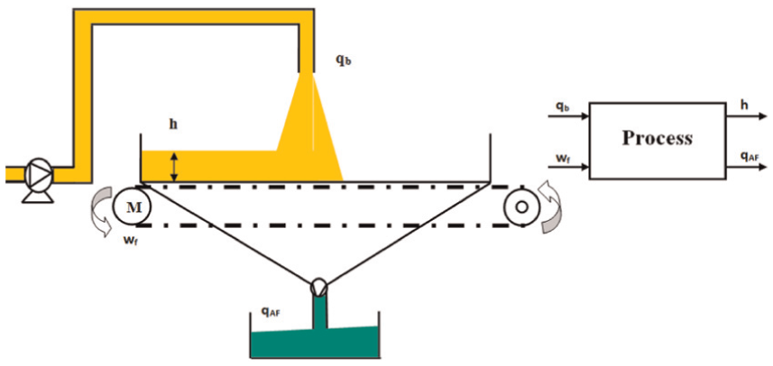
The flowchart and the block diagram of the filter.
The mass of the slurry injected from the reactor to the filter

where
After filtration, the mass of the slurry in the filter

The mass of the filtrated acid

where
Substituting (2), (3) and (4) into (1), we get

If we divide (5) by

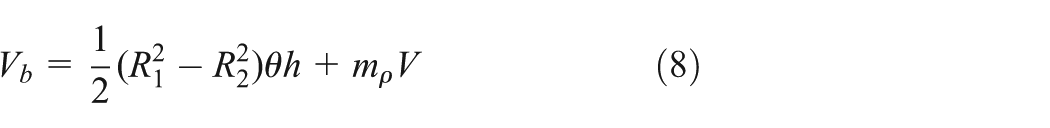
The filter has the shape of a ring with external radius
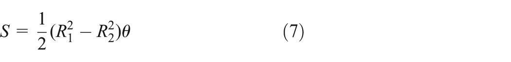
we introduce (7) into (6), we obtain
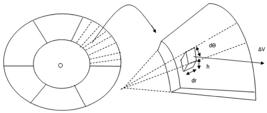
Decomposition of a filter cell.
If we differentiate with respect to time, we obtain
In fact, the angular deviation with respect to time
We take
Finally we get
Calculation of the flow rate of the phosphoric acid equation
To describe the flow of a fluid through a porous medium, we use Navier–Stokes law and Darcy’s law. Darcy’s law is a relation between the flow of a fluid and the loss of charge (Chassagne, 2010). The mass conservation equation coupled to the fluid motion equation gives the incompressible Navier–Stokes equations. The main unknown parameters in this equation are the mass density, the velocity, the pressure, and the temperature, but this list could be longer depending on the case studied. The purpose of this part is to describe the corresponding fundamental solution for the equations of an incompressible fluid model (Thomann and Guenther, 2006). The Navier–Stokes equation, on the other hand, has received renewed interest provided by the clay mathematics institute (Peter, 2015). The Navier–Stokes equation is

with
P: pressure;
t: time;
where
If we multiply equation (13) by S, we obtain
Then if we take
Now, we want to search for the following two terms
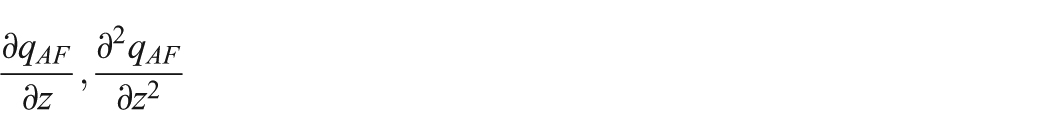
To find these two terms, we must use Darcy’s law. The flow of the strong acid is characterized by a flow rate
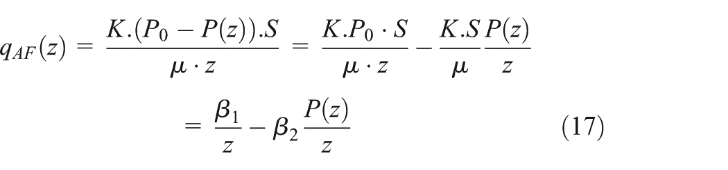
with
If we differentiate the previous equation, we obtain
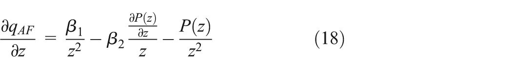
If we differentiate equation (18), we get equation (19)
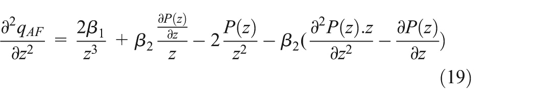
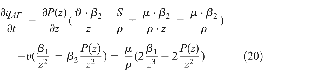
If we substitute (18) and (19) into (16), we find
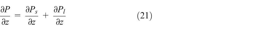
The overall pressure P in the slurry mixture is the sum of the pressure of the solid pressure

The differential of the pressure with respect to the z-axis is as follows
The expressions of
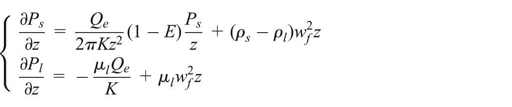
with
E: ratio of lateral and normal stress (dimensionless)
So, the overall pressure is the following
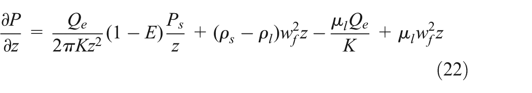
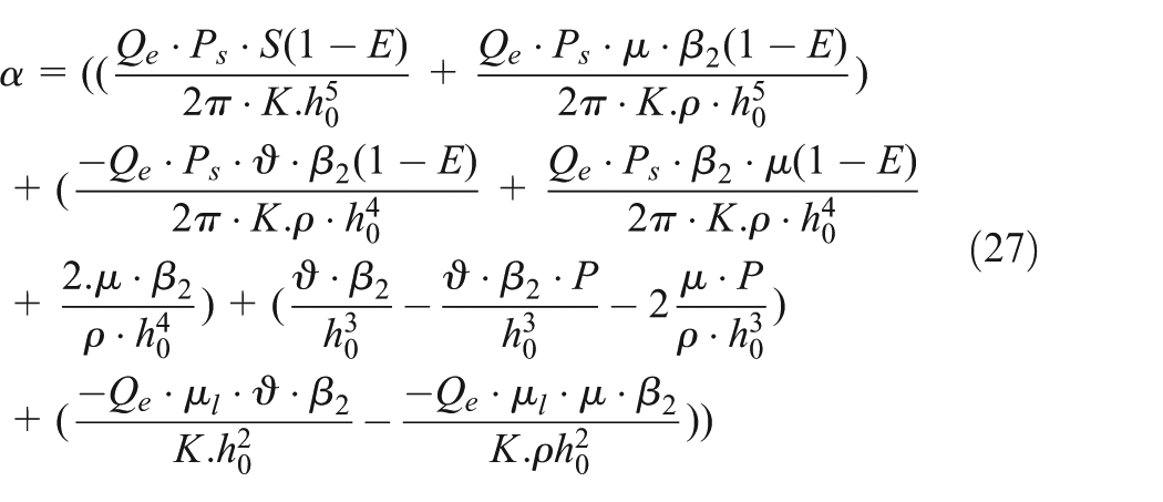
If we replace
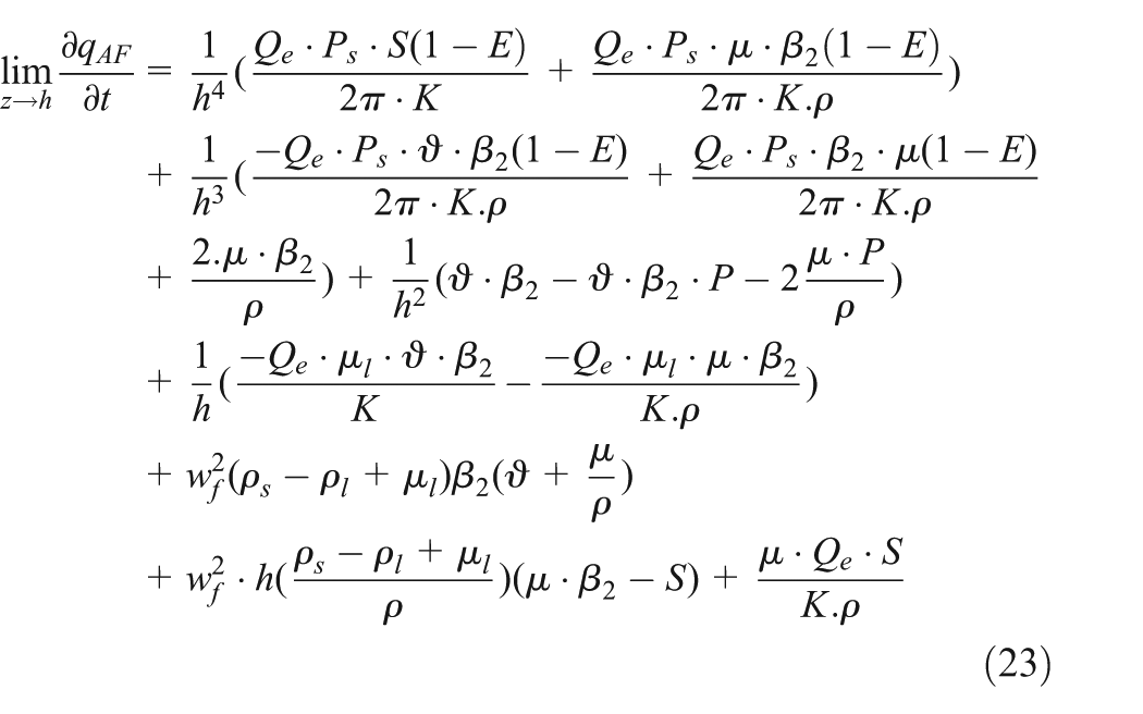
Finally we get

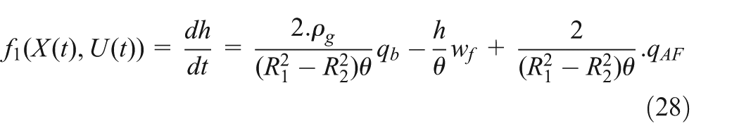
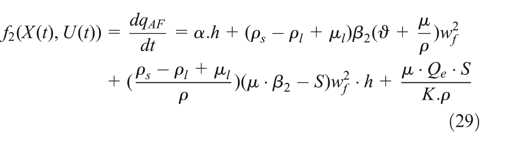
The 1D nonlinear model of the rotary drum filter
Finally, the nonlinear model obtained is as follows
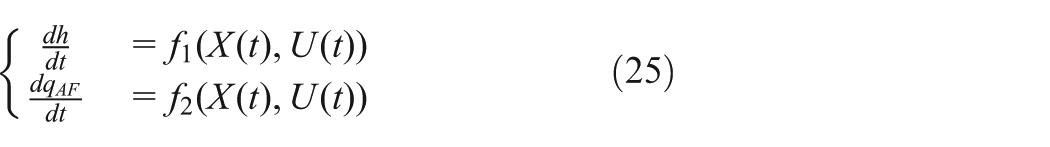
where
The nonlinear equation systems implementation brings changes onto the evolution of events of industrial system that can not be addressed like linear systems. For controlling such systems, it is quite necessary to take into account the nonlinear phenomena.
The simulation of the non linear system gives the two following outputs:
the height of the cake h (m);
the volume flow rate of the strong acid
We note that the thickness of the cake increases over time until it reaches a value of 0.06 m, similarly the volume flow rate of the filtrate which increases to a value close to 74
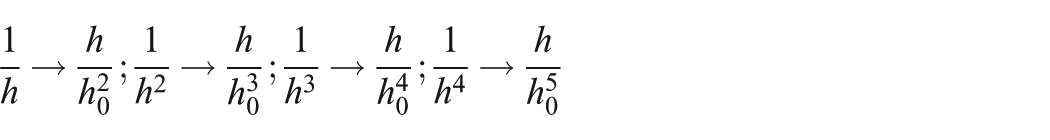
Linearization of the 1D model of the rotary drum filter
In this section, we use linearization around an operating point
We will linearize the following terms:
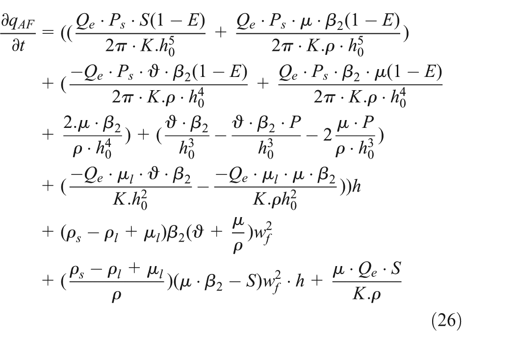
We make a linear approximation with the first order Taylor’s formula for h
where
So, we obtain
We suppose that
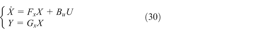
So the linear model of the rotary drum filter is given by the two following equations
The equations of the model include the product of a state variable and a control variable. In order to linearize the model, we must use Jacobian linearization.
We will select an operating point at steady state
Moreover, if we suppose that
where
At the steady state we have
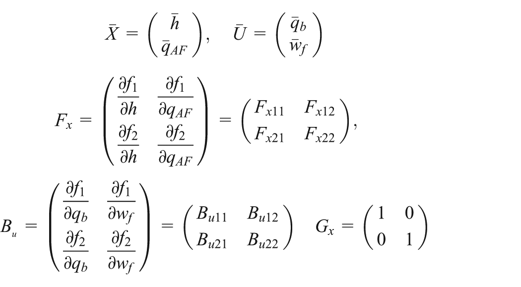
with
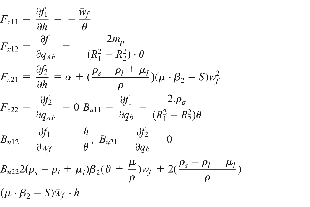
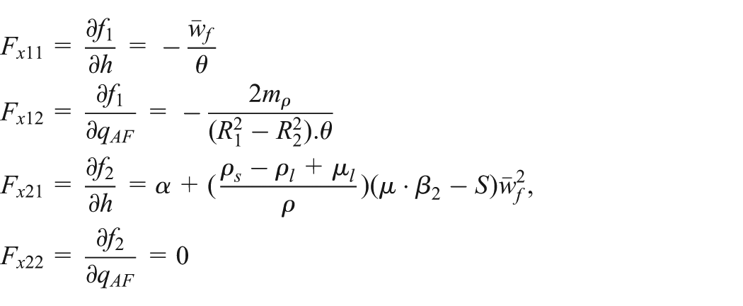
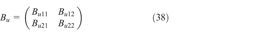
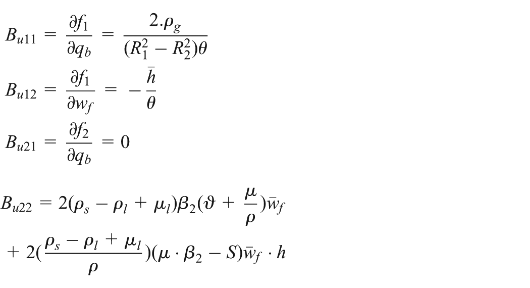
So, the final Jacobian matrices of the state space are

Simulation results and validation of the model
The simulation is carried out by “MATLAB” which is among the most developed software for the simulation of production systems. We suppose that the rotary filter on the Tunisian Chemical Group (TCG) is a multi-input/multi-output nonlinear system, which has like inputs and outputs:
In order to investigate the filter and its changing states, our system was modelled with the intervention of the disturbances. By this method, we can get closer to the real system.
Validation of the model is the process of determining the degree to which a simulation model and its associated data are an accurate representation of the real world. The factory is supervised by the SCADA system in which all the experiments and measurements are taken directly from the SCADA database. These control and output measurements are mentioned respectively as U and
Figure 4 shows the control inputs of the system. These inputs refer to the flow rate of the slurry
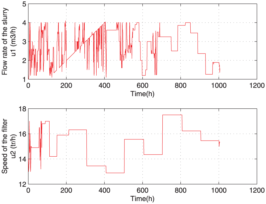
Evolution of the inputs of the filter.
Figure 5 presents the output
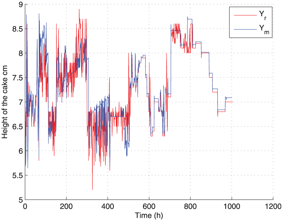
Representative figure of the real and the estimate output (height of the cake).
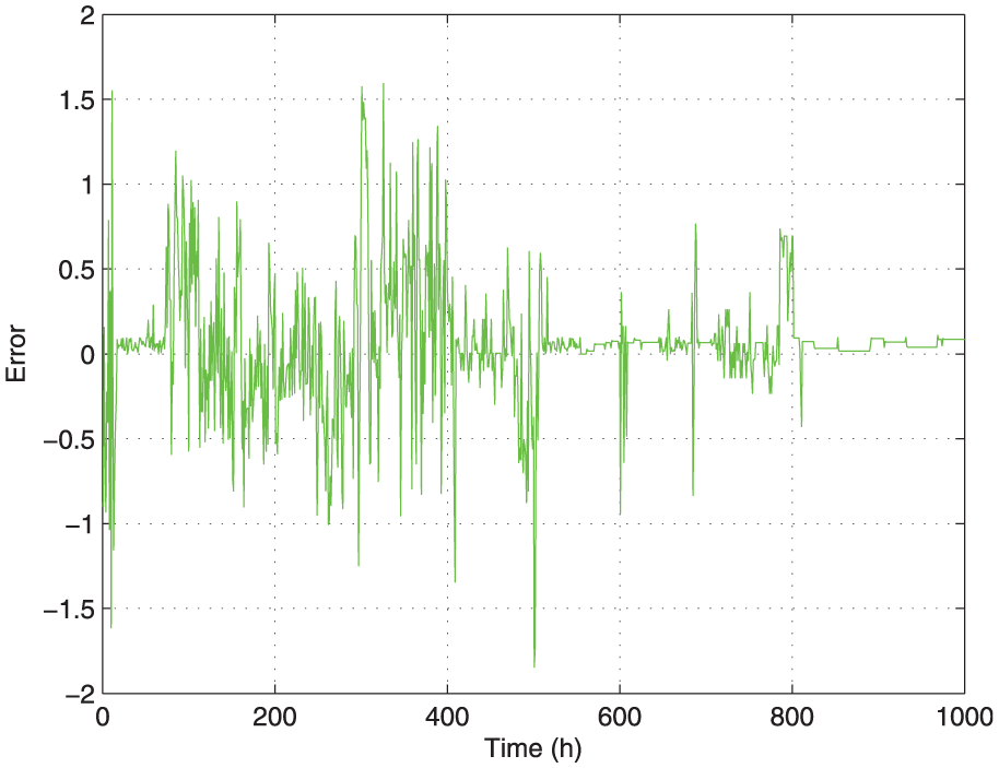
Representative figure of the error of the estimate output (height of the cake).
Figure 7 describes the output
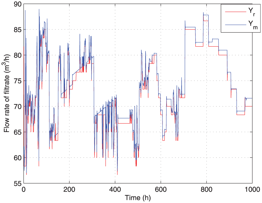
Representative figure of the real and the estimate output (flow rate of filtrate).
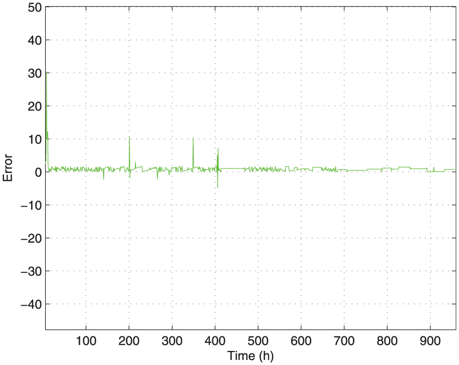
Representative figure of the error of the estimate output (flow rate of filtrate).
We note that there is a gap between the real output and that of the model, this difference is due to the errors on the estimated model resulting from insufficient excitement. So it’s a problem of excitation.
2D modelling based on FM-II method
Implementation of the FM-II method algorithms
Consider the linear 2D system described by the following FM-II model (Fornasini and Marchesini, 1976)

where
The two dimensional linear system is said to be asymptotically stable if the definition 1 in Kaczorek (2006) is checked.
The 2D system is asymptotically stable if there exist matrices
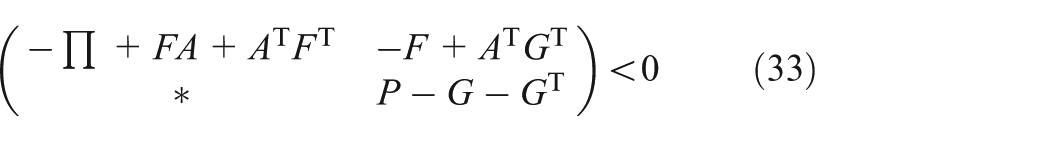
where
the transfer matrix of the previous model is:
write


with
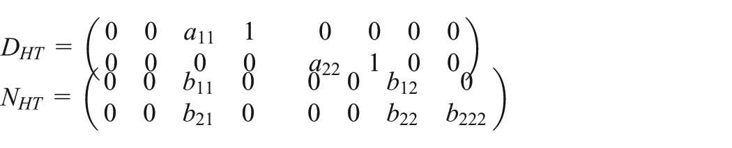
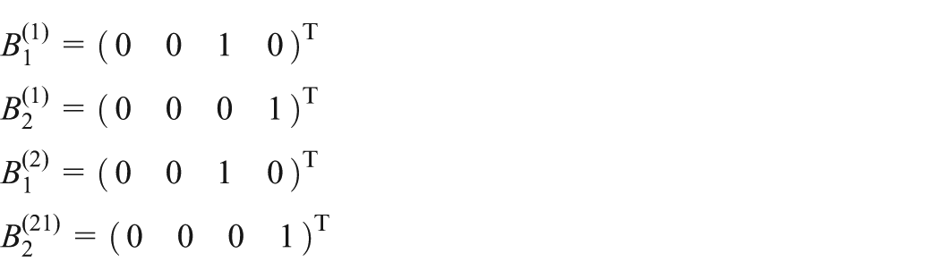
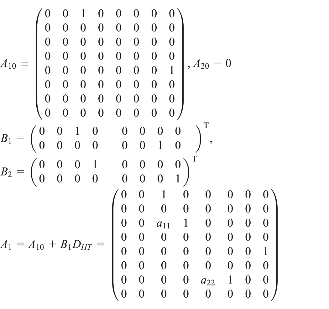
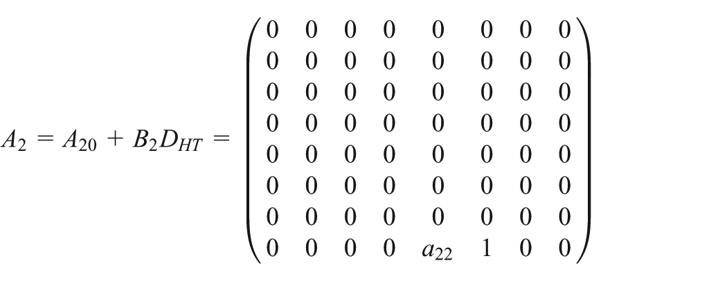
construct the matrices

the realization is finally obtained as
By thoroughly investigating the structural properties of FM-II model, we found that to meet the relations specified in (42), (43), and (44) so that a realization can be obtained.
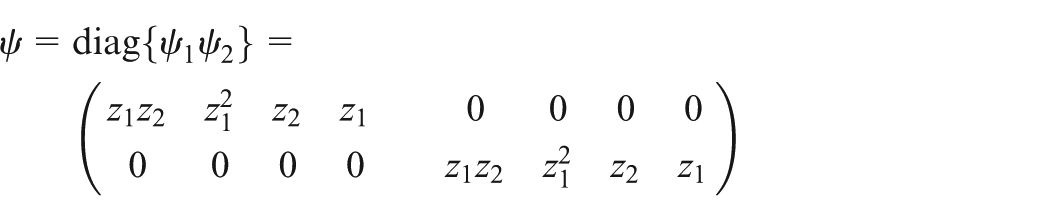
ψ has to satisfy the following conditions.
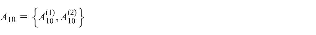
Let
The above realization procedure produces a state space description (
Starting from the initial
Once
where
Therefore, we have
2D modelling of a rotary drum filter
Calculation of the transfer matrix
The state vector is
with
The command vector is
with
At first, we calculate the determinant of
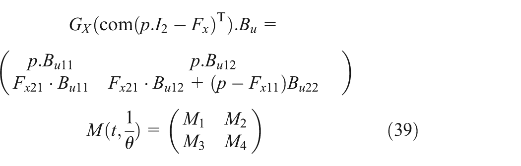
with
We have
So
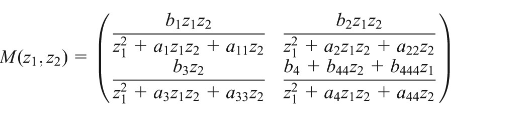
with
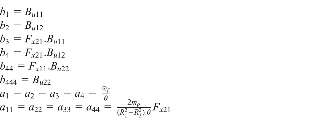
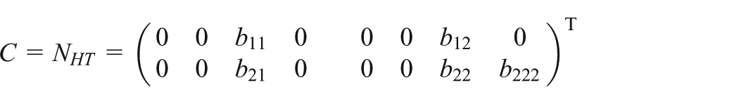
From the transfer matrix we can formulate the following matrices
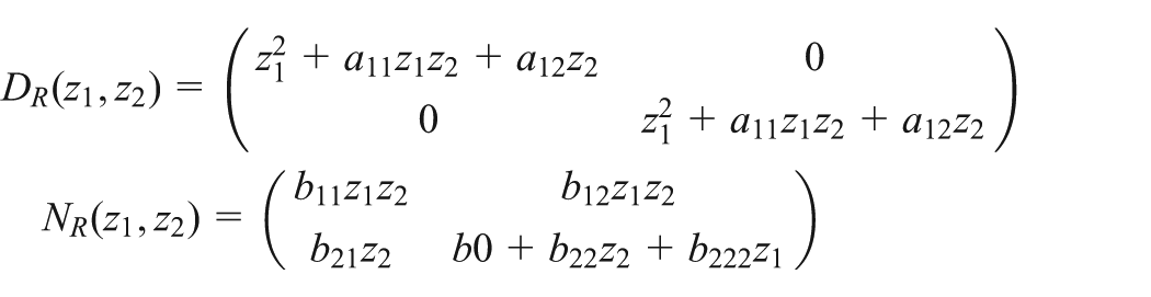
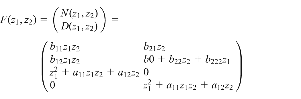
Thus the column degrees of columns 1 and 2 in
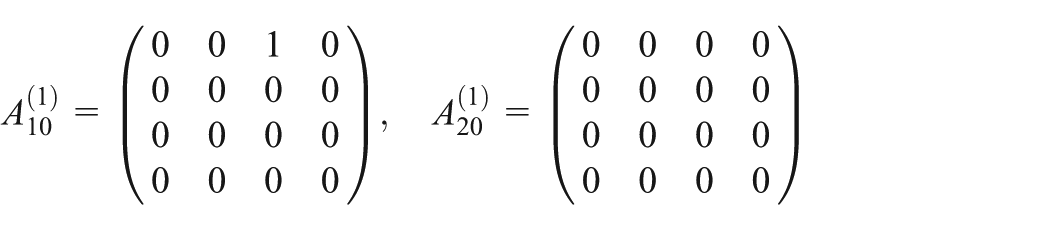
Apply now Algorithm 1,
So, for
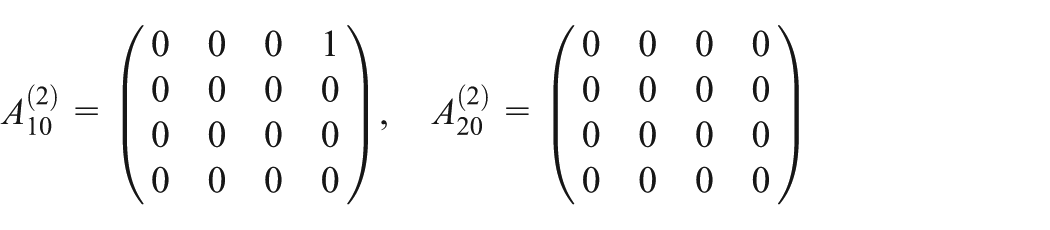
For
Since only
Calculation of
and
On the other hand, for
It is easy to obtain
Since
Conclusion
In this research a two dimensional model was proposed to describe the dynamic behaviour of a rotary filter, which works in a permanent regime and it is dedicated to the aspiration of various types of acid: strong, medium, and weak. This method is considered among the most complex, multi-variable, and unstable systems on an industrial scale. Therefore, its study requires deep research in order to know all of the parameters that have an influence on the normal operation of the filter. Using the parameters that characterize the “AOUSTIN-UCEGO” filter, we find a two dimensional model for the filter. A constructive state-space realization procedure has been used for 2D systems which may produce an FM-II local state-space model.
Footnotes
Acknowledgements
This work was carried out in the Tunisian Chemical Group (TCG), SKHIRA factory in the unit of the phosphoric acid production.
Funding
This work was supported by the Ministry of the Higher Education and Scientific Research in Tunisia.