






Abstract
This paper focuses on a challenging problem in the internal model control (IMC) strategy: the model inversion to design the IMC controller for non-square systems. Several existing approaches for the synthesis of a specific inversion of the identified model will be presented in this paper to deal with the differences between the system’s inputs and outputs numbers. The non-square effective relative gain is firstly presented. It consists of the measurement of interactions between the loops of the system in order to square the system and make it invertible. The equivalent transfer function method is presented as well. It is based on tuning the pseudo-inverse of the process to design the internal model controller. These methods are then compared with a novel proposed model inversion approach based on virtual outputs method. Virtual adding is considered in order to obtain an invertible square transfer matrix to design the internal model controller. This simple yet effective method ensures robust control performance. Its efficiency and availability, as compared with other presented methods, is illustrated through simulations on an overactuated system with three inputs/two outputs.
Keywords
Introduction
Processes having multiple inputs and multiple outputs (MIMO) occur frequently in the modern complex industrial fields. They can be partitioned into square and non-square systems (Moro and Bonavitat, 1997). Processes with equal number of inputs and outputs are called square systems. Non-square systems are then referred to unequal number of inputs and outputs processes (Ben Omrane et al., 2012; Jin et al., 2014; Qibing et al., 2009; Quan et al., 2012). The control of such systems is challenging due to the existence of interactions among input and output variables.
Several researches have been done in the control field of non-square systems. A simple control method consists of squaring non-square systems by adding or eliminating the appropriate number of the input or output variables. However, this control method may lead to an increase of the control cost when adding variables or reduced control performance when removing inputs or outputs, due to neglected dynamics (Chen et al, 2011; Rao and Baram, 2006; Reeves and Arkum, 1989).
This paper deals with the synthesis of the internal model control (IMC) designed for non-square systems. This control strategy is considered as an excellent vigor to settle the control problems of MIMO systems due to its simple design, strong robustness, and its good tracking ability performance (Ben Omrane et al., 2012; Qibing et al., 2009). The IMC incorporates a model of the system. The Tuning of the IMC controller corresponds to a specific inversion of an appropriate identified model, since direct inversion is rarely achievable. Considering non-square systems makes the IMC controller design much more complicated, as it cannot get the traditional sense of inversion (Fossard, 1972; Dhahri et al., 2016; Qibing et al., 2012).
Some available results in literature consider several model inversion methods to design the IMC controller for non-square systems. The pseudo inverse method can be considered to inverse the transfer matrix of the non-square model. However, the application of this method may be difficult and very complicated.
The non-square effective gain (NERGA) method is as well proposed in Quan et al. (2012) to inverse the transfer matrix of the model. This method is considered as a criterion to choose a square subsystem from a non-square system by adding or removing appropriate inputs or outputs. Once the system is squared, controller synthesis procedures based on the IMC strategy, developed for square systems, are applied directly. In Pavarati and Subbulekshmi (2011) and Luan et al. (2014), the equivalent transfer function (ETF) method were proposed to design the IMC controller by approximating the pseudo-inverse of the non-square process in a simple and easy way. In this paper, a novel inversion approach based on virtual outputs (VO) method is proposed. It consists on attaching lines to the non-square transfer matrix of the model in order to square it. This virtual adding aims to obtain a square transfer matrix and have no influence on the response of the system (Fossard, 1972).
In the present work, the control performances of non-square effective relative gain, ETF and VO methods for inversion the model process to design the internal model controller for non-square systems are evaluated and compared.
This paper is organized as follows. Section 2 describes the internal model controller design for non-square systems and explains the proposed model inversion methods. Section 3 shows simulation results with concluding remarks in section 4.
IMC design
In this section, we present the IMC. On the one hand, we describe its basic principle and its properties. On the other hand, we present the structure of the IMC controller as well as the study of its stability. Finally, solutions for the problem of inversion are presented. They aim to design a controller that is easy to carry out and close as possible to the model inverse (Yaman et al., 2016).
The IMC structure
The block diagram of IMC structure for a multivariable system is exposed in Figure 1 (Chu et al. 2018).

Structure of IMC.
Where: G(s) is the transfer matrix of the process with “m” inputs and “n” outputs; CIMC(s) is the internal model controller designed to control the process G(s); M(s) is the process.
Considering the case of perfect modeling, so we have G(s) =M(s). From Figure 1, the following equation can be derived for nominal systems
Where Im is the identify matrix
The closed-loop system shown in figure 1 is internally stable if and only if all four elements of the matrix in (1) are stable.
The internal model controller design
The IMC controller designed for multivariable systems presenting or not multiple time delays and / or with a non-minimum phase shift is presented by Figure 2 (Dhahri et al., 2016).
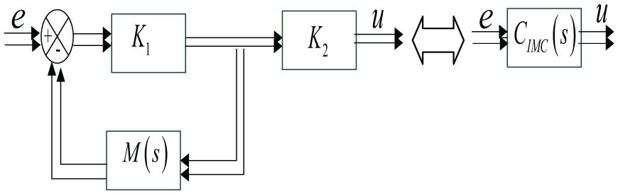
Generalized multivariable controller structure.
In order to ensure good control performance and tracking feature, the IMC controller must satisfy the following equation
From Figure 2, the closed-loop transfer matrix CIMC(s) between e and u is derived as follows (Dhahri et al., 2016)
where K1 is the inversion matrix of the form
In steady state, the gain matrix K2 is written in the following form
where M(0) is the of static gains matrix of the model M(s).
The gain matrix K2 aims to compensate the static errors of the system, while K1 is chosen in order to ensure the stability of the controller and to achieve the inverse of the model M(s).
On the basics of the IMC principle, the synthesis of a controller equal to the inverse of the model transfer matrix ensures perfect tracking and good control performances. Nevertheless, the inversion in a direct way is practically impossible, especially for non-square systems. To overcome this problem, several methods of non-square model inversions are proposed and developed in the next sections.
Model inversion using NERGA method
This method is based on the analysis and pairing the loops in order to overcome the singularity of system transfer matrix (Xiong and Jian, 2006). The non-square effective relative gain array “NERGA” is recognized as a spread of relative gain array “RGA”. The RGA has proved its ability to choose the input-output pairing for diagonal control design by illustrating the intensity of coupling within the different process loops and exhibiting the impact degree of each loop by other circuit (Shinde et al., 2015). The NERGA corresponds to loop pairing criterion by employing the steady-state gains and bandwidth of the non-square process transfer function elements.
Consider a non-square system with “n” rows and “m” columns, presented by the following process transfer function matrix G(s)
The gij(s) presents the process transfer function element linking the ith input and jth output.
The effective gain matrix EG(s) (Quan et al., 2012) is given by the following expression
where: G(0) the static gain matrix and Ω the bandwidth matrix are expressed as follows (Quan et al., 2012; Xiong and Jian, 2006)
and
where
We report that the operator ⊗ is the Hadamard product. It consists on applying an element by element multiplication.
The effective relative gain ψij(s) between the output yi and the input uj is given by the ratio ψij = eij/ êij. The term êij indicates the effective gain between yi and uj when other loops are closed (Chang and Yu, 1990; Xiong and Jian, 2006).
Once the gains of all the existing combinations between the various inputs and outputs of the system are calculated, we can obtain the NERGA matrix defined by formula (9)
where EG and
Throw the non-square effective relative gain matrix, the sum of the elements in each row and column, respectively noted by RS and CS, can be calculated and expressed as follows
For overactuated systems (m>n), the sum of elements in each row RS is equal to 1, and the sum of elements in each column CS is between 0 and 1. If CS(i) is adjacent or near to null, the ith input loop admits a small impact on the output loop. Thus, the corresponding loop can be easily overlooked and consequently deleted. In the other case, if the process is under-actuated (m<n), the sum of elements in each column CS is equal to 1, and the sum of elements in each row RS is located in the interval [0 1]. If RS(i) is near to zero, the ith input loop admits a little impact on the output loop. Consequently, this loop can be neglected and removed from the system (Quan et al., 2012; Schaper et al., 1999; Xiong et al, 2005).
Model inversion using ETF
The equivalent transfer function (ETF) method has been developed to approximate the inverse of the process transfer matrix based on the measurement of dynamic interactions of non-square systems (Jin and Jiang, 2013; Jin et al., 2014).
The majority of the industrial systems are processes of second order plus dead time (SOPDT). The SOPDT transfer function is described below
The ETF is given by equation (13); it takes into account loop interactions
The expression of the pseudo-inverse of non-square process
where
The basic steps required to obtain ETF for a non-square system, are given by the following algorithm.
Algorithm ETF
❖
❖
The NRGA between output yi and input variable uj is defined as the ratio of two gains representing,
The NRGA in matrix form is defined as follows
where
❖
The NRNGA can be calculated as described below
where
where
The normalized gain matrix
where
❖
The NRARTA can be calculated by
where
❖
The gain of the ETF matrix is defined as follows
The time delays of the ETF matrix are expressed as described below
The obtained ETF matrix serves to evaluate the internal model controller.
The IMC controller (Jin et al., 2014) is calculated as follows:
where
F(s) is a low pass filter. It ensures the realization of the IMC controller. The parameter
The mathematical description of
where
A filter
The first order filter
where
Model inversion using VO method
Over-actuated systems are multivariable systems with more control inputs than outputs. As a result, the transfer matrix of an over-actuated linear system is not square. The model M(s) must be chosen very close to G(s) the process transfer matrix. The controller CIMC(s) is chosen as an approximate inverse of the model. The idea consists on squaring the model to be inverted and then eliminating excess outputs that will be released to the system.
A new inversion technique of the model M(s) by means of the VO is proposed. It consists on attaching lines to the non-square transfer matrix of the system G(s). This virtual adding aims to obtain a square transfer matrix, which allows the inversion operation. The excess outputs are then eliminated from the system.
To maintain the original performances of the studied system, we have to remove the added variables through the programmation part. The VO are only used to square the model transfer matrix (Foassard, 1972).
Once the VO method is applied, we can now deal with a non-singular matrix. This method is more effective for non-square model inversion as compared with the pseudo inversion that can give several solutions and the controller remains unsuitable.
For overactuated systems, the VO amount is referred to a transfer matrix of dimension ((m-n), m).
The studied overactuated system can be shown through equation (32)
In order to simplify the study and to avoid inversion problems, the new ((m-n), m) transfer matrix that contains the added variables transfer matrix can be chosen as first-order transfer functions or constants satisfying the stability criterion. It is presented as follows
The proposed IMC structure proposed in Touati et al. (2013) for square multivariable systems is then modified in order to eliminate the excess (m-n) outputs. A block called (elimination of (n-m) outputs) is inserted into the basic IMC structure (cf. Figure 1). The aim of this block is to eliminate the (m-n) excess outputs by means of the usual logical operators, as depicted in Figure 3.

The elimination of (m-n) outputs block.
The new IMC structure of multivariable over-actuated system is then shown in Figure 4.

The IMC structure for overactuated systems.
Study of the stability of the controller
The IMC controller CIMC(s) expressed by equation (3) can be reformulated using the state space representation as follows
where:
The stability analysis can be processed by the knowledge of the state matrix Ac, which depends of the gain matrix K1.
In this paper, the Lyaponov method is considered to study the controller stability (Maamri et al., 2006).
The stability condition highlighted by Lyapunov stability theory requires that the system (34) is stable if and only if there exists a positive definite matrix
This work is restricted to the use of the Linear matrix inequality technique to study the stability of the internal model controller and to calculate the range of the gain K1 that ensures the stability of the open loop system (Adelipour et al., 2014).
The resolution of an LMI problem with Matlab version 2012a is presented according to the following algorithm:
First, we initialize the controller matrix Ac.
Second, we start to describe and initialize the LMI description.This is easily done by the function
Then we indicate,with the function
In the next step, we indicate the different terms that make the LMI depending on whether they are constant or that they answer for P. We define our LMI :
The final step, before launching the numerical resolution, consists on indicating that the definition of the problem LMI is finished, and that the function is feasable by the corresponding solver
Solver for LMI feasibility problems is L(x) < R(x). This solver minimizes t subject to L(x) < R(x) + t*I. where L(.) and R(.) are affine functions of some structured matrix variables x1,…, xn. A simple example is the Lyapunov inequality defined by equation (35).
The best value of time t should be negative for feasibility simulation results. The equation (34) is stable in the sense of Lyapunov.
Simulation results
In order to underline the interest and the performance of the proposed approaches, the air path of a turbocharged diesel engine (Lamara et al., 2012) is considered. This overactuated system is 4 cylinders with 2 liters and 80.9 KW. The three pneumatic air path actuators are wastegate (WG), EGR valve (EGR) and intake throttle (TH). The air path system of the turbocharged Diesel engine is described by the Figure 5 (Lamara et al., 2012).

Air path scheme of a turbocharged Diesel engine with Exhaust Gas Recirculation (EGR).
The dynamics representation of the air path of a turbocharged diesel engine, with three inputs (EGR, TH and WG) and two outputs (QAir and PCol), is given by the following transfer matrix (Lamara et al., 2012)
The eigen values of G(s)
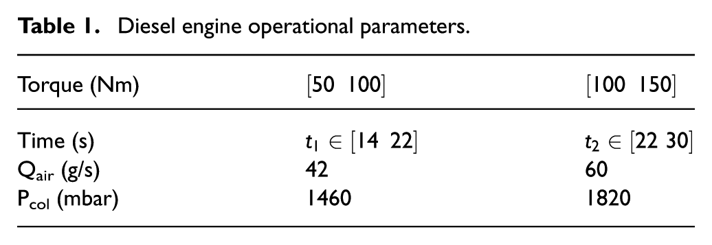
The simulation study is considered for a four-cylinder diesel engine speed of 3000 rpm, according to the parameters described in Table 1.
Diesel engine operational parameters.
Internal model controller design based on NERGA
Starting with the application of the non-square effective relative gain array (NERGA) approach. The (2×3) system is squared down to a (2×2) system as we can delete either an input or an output that has a little effect on our process.
To obtain the effective gain matrix of our system, we should firstly calculate both static gain matrix G(0) and the bandwidth matrix Ω presented by the following equations
Using the Hadamard product, the effective gain matrix EG is equal to
Throw the formula (9); we obtain our NERGA expressed by:
Once the NERGA is evaluated, we can now calculate the sum of the elements in each row and column.
As the third input loop is now deleted, the new square transfer matrix describing the system is expressed as shown below
Thus, the new non-square effective relative gain array is calculated as
We can obviously claim that the coupling problem between the different input and output loops has disappeared.
Consider the case of imperfect modeling. So,
The eigen values of M(s)
The application of the LMI approach allows us to deal with quadratic stability of the internal model controller
The gain interval K1 ensuring the stability of the controller is given by
For the studied system, two chosen gain matrices K1 are considered:
Figures 6 and 7 display, respectively, the system control actions (EGR and TH)) and system outputs (Qair and Pcol ) for

Evolution of process control actions and outputs for NERGA-IMC approach for

Evolution of process control actions and outputs for NERGA-IMC approach for
It can be seen that the proposed control low ensures an accurate system. The system outputs Qair and Pcol have good tracking features. However, the output Qair presents a relatively important overshoot due to the negative gains of the model. The control action EGR presents a small overshoot for
Internal model controller design based on ETF
This section is dedicated to the ETF approach. First of all, we will start with the resolution of the ETF algorithm to design the internal model controller. Then, we will apply this algorithm for the studied system to test its robustness and performance.
The steady-state gain of the system G(s) is given as follows
The time delay of the system is given below
The average residence time array is obtained as
Thus, the non-square RGA is
The non-square RNGA is calculated as follows
The non-square relative average residence time array is obtained as
According to the previous results the ETF parameters are
Using the above results and equation (15), the ETF matrix is calculated below
The filter time constants can be chosen as:
Hence, the feedback filter is
Finally, a stable IMC controller can be obtained from equation (28). It is represented by the following transfer matrix
Figure 8 displays the system inputs and outputs evolution. Set-point tracking is established for both outputs. However, important overshoot in Qair response is noticed. It can lead to serious problems for real time implementation, despite the fact that it is gradually diminished due to the feedback loop. The Pco response presents as well a slower tracking feature as compared with the results obtained for NERGA method.

Evolution of process control actions and outputs for ETF-IMC approach.
So, the application of the ETF-IMC method has reduced control performance as compared with the NERGA method.
Internal model controller design based on VO
Dealing now with the new VO method proposed in this paper, and applied to the same system studied previously.
The model M(s) is chosen close to the process G(s). For our case the process G(s) is of dimension (2×3). The VO method considered for this overactuated systems, consists on adding ((3-2), 3)) vector to the original transfer system in order to square it.
The model M(s) is then chosen of dimension (3×3) so that it can be invertible. The elements of the transfer matrix M(s) are the same as G(s) and we will add a third line to the matrix G(s). The elements of this line are transfer functions with fast responses and do not influence the process G(s).
The chosen transfer function matrix of the model is given by the following matrix
The eigen values of M(s)
Solving the LMI in equation (34) for M(s) given by the equation (60), we obtain a matrix P of dimension
For the studied system, two chosen gain matrices K1 are considered:
Figures 9 and 10 display, respectively, the system control actions (EGR, TH and WG)) and system outputs (Qair and Pcol ) for

Evolution of process control actions and outputs for VO-IMC approach for

Evolution of process control actions and outputs for VO-IMC approach for
The system outputs present good accuracy properties, smaller overshoot and have faster tracking features for
Comparison analysis
Once the three inversion methods: NERGA, ETF and the VO, are evaluated, a comparative study seems to be interesting to demonstrate and to compare their efficiencies.
In this section, the air circuit is subject to set point changes. QAir is regulated at 42 g / s and 60 g / s, respectively, during the two time ranges
The response time of 5%, evaluated for the three inversion techniques, gives a good evaluation of the speed of a system; it expresses the time taken by the system subjected to a step to reach its steady state value within ± 5%. We note that the NERGA-CMI structure and VO-CMI have better performance in terms of response time versus ETF-CMI, as shown in Table 2.
Quantitative comparison between IMC Controller based on NERGA, ETF and VO method.
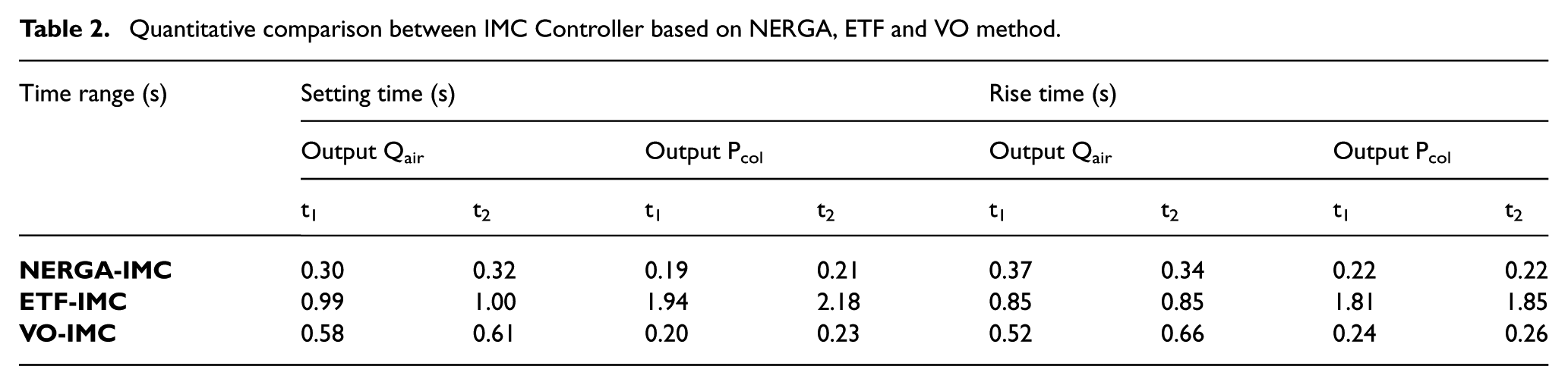
The performance index for the transient regime is evaluated by calculating the rise time of the air circuit, which represents the time taken by the QAir and PCol outputs to go from 10% of their final values to 90% of their final values. The NERGA-CMI method performs better than other approaches in terms of climb time, as shown in Table 2.
However, the NERGA-CMI structure is not always applicable, especially when the sum of elements at each row and column are close. So, we cannot delete an input that does not affect the system to make it square. This operation may lead to performance degradation due to the elimination of certain information.
We note also that the ETF-CMI airflow outputs converge to set points with slow response and rise times as compared with the virtual output and NERGA-CMI method. This method requires a long calculation time that complicates the implementation in real time. In addition, the response of the Qair output presents some relatively high peaks, as shown in Figure 7. Besides, the ETF-CMI method presents a problem in the choice of the filter, which requires an adequate knowledge of the G (s).
The proposed VO approach overcomes these difficulties. It has good rise time and response, an accurate response, does not require the use of filters and the elimination of system inputs. This new simple yet effective method leads to better control system performances.
A comparison between the IMC control based on VO method and the decentralized crone control (Oustaloup, 1991) can be proposed. It aims to show the effectiveness the proposed IMC strategy as compared with crone control.
The decentralized crone control strategy is based on fractional-order differentiation (Oustaloup, 1991). The aim of the CRONE strategy for MIMO systems is to ensure robustness of the closed-loop matrix dynamic by maintaining the damping or resonance factors (Oustaloup, 1991). The crone control can manage the robustness/performance tradeoff.
For the proposed system, the decentralized crone controller K(s) is described by the transfer matrix below
Figure 11 illustrates simulation results for this scenario.

Evolution of process outputs for VO-IMC approach and decentralized crone control.
The comparison between the IMC strategy and the decentralized crone control shows the benefit of the IMC strategy. It ensures better dynamic performance, smaller overshoots, and smaller settling time.
Robustness of the VO-IMC approach towards external disturbances
In order to test the robustness of the IMC controller based on VO method, it is proposed to disrupt the system by applying a white noise of amplitude 3 for Qair and Pcol between 18s and 25s. Figure 12 illustrates simulation results for this scenario.

Evolution of process outputs for VO-IMC approach in the presence of disturbances.
It can be seen that the system remains stable and the disturbance is completely rejected. The IMC controller based on VO inversion approach is able to compensate these disturbances. This fact confirms its robustness.
Robustness of the VO-IMC approach towards parameter uncertainties
The test of the controller robustness allows us to check whether the IMC control based on the VO method is capable of compensating the uncertainties on the air path system parameters.
Figure 13 displays the evolution of the system outputs for an uncertain transfer matrix

Evolution of process outputs for VO-IMC approach in the presence of uncertainties.
We notice that despite uncertainties, set-point tracking is established with acceptable performance of accuracy, speed, and stability. This fact, confirms the IMC–VO strategy robustness towards uncertainties. It should be noted that when increasing uncertainty amount, the system becomes slower and the overshoot is greater.
The IMC control based on virtual outputs approach can be easily implemented in real time and the gains K1 and K2 remain the same despite uncertainties.
Conclusion
In this paper, we have been interested in the comparative study of several inversion methods for IMC controller design proposed for non-square systems.
The proposed process inversion methods are NERGA, ETF and a new proposed approach, namely virtual outputs method. They were applied on an overactuated system with two outputs and three inputs. A comparative analysis was proposed. It shows clearly the efficiency of the virtual outputs method and its ability to avoid the complicated calculation, such the matrix inverse. The obtained controller is simple, has few tuning parameters, is easy to implement in industrial processes and presents good control and robustness performances.
Footnotes
Declaration of conflicting interests
The author(s) declared no potential conflict of interests with respect to the research, authorship and/or publication of this article.
Funding
The author(s) received no financial support for the research, authorship, and/or publication of this article.
