Decentralized robust evolving cloud-based controller for two input two output systems

Abstract

The fuzzy logic controller (FLC) makes it possible to control a system using IF-THEN rules through human intellect. It tackles parameter uncertainty using imprecise reasoning. The fuzzy logic controller is usually tuned using offline methods. An online evolving adaptation of fuzzy controller design is a recent trend in fuzzy rule-based systems. The robust evolving cloud-based controller (RECCo) is one such controller implemented for single-input-single-output (SISO) systems. The membership functions and consequent rules are automatically updated in real time based on the input data. In this paper, a decentralized robust evolving cloud-based controller (DRECCo) is proposed for two-input-two-output (TITO) systems. It consists of two independent loops with RECCos having a nonparametric premise facet and an adaptive proportional-integral-derivative (PID) model consequent facet. The effectiveness of the proposed method is validated for the benchmark interacting two-tank process (ITTP) and quadruple-tank process (QTP) by simulation and in real time. The results indicate that with the information of loop pairing and the forward-acting/reverse-acting nature of the process, the proposed controller can adapt itself to ensure set-point tracking and disturbance rejection.

Keywords

Decentralized robust evolving cloud-based controller (DRECCo)adaptive control decentralized cloud-based controller evolving fuzzy type control ANYA fuzzy-based control

Introduction

Many systems available in multiple industries are of the multi-input-multi-output (MIMO) type. The control of a MIMO system is complicated because of the interaction between the regulated and the manipulated variables. Fuzzy logic controllers (FLC) have achieved substantial success in the past decades because they can operate with imprecise models and can imitate human-like decision-making. Mamdani and Takagi Sugeno (TS) are different forms of fuzzy rule-based (FRB) systems (Ross, 2010). The main advantage of fuzzy logic is the ability to convert human intelligence into a sequence of logical rules. A sequence of IF-THEN rules should be specified for designing a fuzzy logic controller. Designing membership functions and writing rules for complex processes is difficult. Even when the developers are familiar with the use of linguistic variables in stating rules, the rules specified while designing may lead to problems such as the following:

Developers may set the rules, but they are not effective.

Information may have to be updated at runtime.

The intelligence given for a rule may be exact, but it may be inexact for another operating condition.

The rules established by the developer could mislead the performance of the fuzzy logic controller at the output stage.

Cara et al. (2010) and Cara et al. (2011) proposed an online adaptive fuzzy controller that uses input-output information to update the membership function and rules of the fuzzy controller. This approach provides a way to obtain self-evolved FLC when the knowledge of plants is not or partially available.

The fuzzy membership of a data sample is correlated with more than one set of data clouds with contrasting membership grades that have been established by spatial density in all data cloud samples. The conventional approach uses predefined and predetermined membership functions, such as sigmoid, trapezoid, and triangle type. In recent machine-learning standards, Cauchy kernels, Gaussian, and others have been conquered until the distribution portrayals deal with the real data density and data distribution. Based on this, a new mechanism of simplified FRB systems is introduced as a substitute for traditional FRB systems. A completely new framework to describe the preceding component is described, which was implemented as the newest class of fuzzy structure, and the preceding part of ANYA fuzzy rule-based (AFRB) system is nonparametric and precisely reflects the actual density and distribution of data (Angelov and Yager 2011, 2012). Table 1 lists the contrast between the typical FRB methods and the proposed one.

Table 1.

Various FRB’s and their dissimilarities.

S. No	Various types of FRB	IF (Premise) part	THEN (Subsequent) part	De-fuzzification
1	Mamdani	Scalar and parametric fuzzy sets	Scalar and parametric fuzzy sets	Centre of gravity
2	TS	Scalar and parametric fuzzy sets	Linear function in general	Weighted sum with fuzziness
3	AFRB System	Nonparametric data clouds	Either of the two forms mentioned above

Costa et al. (2013) introduced the design of a self-evolving first-order controller for a coupled tank based on the ARFB system. A new fuzzy controller that uses an ARFB structure (robust evolving cloud-based controller (RECCo)) was presented in Angelov et al. (2013). The major benefit of the robust evolving cloud-based controller is that the plant model is not required. Skrjanc et al. (2014) enhanced the robust evolving cloud-based controller. The idea is to adjust the basic parameters required by the control algorithm that uses the fundamental knowledge of the regulated process, such as input-output range, sampling time, and time constant. Different real-time situations have been studied by Andonovski et al. (2015a, 2015b) that used absolute values as an updated adaptation law to enhance the performance of the robust evolving cloud-based controller in the initial phase. A newly arrived cloud is incorporated as per the global data density and a smarter way of using localized density thresholds has been discussed in Andonovski et al. (2016a, 2016b), Andonovski and Costa (2017), and Andonovski et al. (2018). Additionally, the preceding component of the AFRB acquires the density across all existing samples of data and is thereafter determined recurrently.

The performance of the robust evolving cloud-based controller was evaluated on an actual heat exchanger and two-tank plants both by simulation and in real time, and a fuzzy and an adaptive fuzzy proportional-integral-derivative (PID) controller were implemented in Bhattacharya et al. (2003) and Kayacan and Kaynak (2009), respectively, for liquid level control. Basci and Derdiyok (2016) presented an adaptive fuzzy controller using a fuzzy identifier to maintain the levels of the liquid for a coupled tank and validated it in a hardware setup to show the interacting dynamics. Musmade and Patre (2013); Zheng et al. (2016); and Zhang and Chi (2020) presented various adaptive controllers such as sliding-mode control, model-free adaptive control, and fractional-order PID controllers. Hajare and Patre (2015) and Mahapatro et al. (2019) described the design of a decentralized PID controller for two-input-two-output (TITO) systems using characteristic ratio assignment and reduced-order model techniques, respectively. Simulations were conducted to validate the applicability of the controller, and it was tested in a practical coupled tank system. The modeling and analysis of four-tank systems for various phases are discussed in Johansson and Nunes (1998); Johansson et al. (1999); Johansson (2000); Astrom et al. (2002); and Zhou et al. (2015).

Studies available in the literature that are related to robust evolving cloud-based controllers have been limited to non-interacting process systems. This paper proposes a decentralized robust evolving cloud-based controller (DRECCo) that extends the application of the robust evolving cloud-based controller beyond non-interacting process systems, that is, an interacting process system. The proposed controller was implemented for two benchmark processes both by simulation and in real time to assess its effectiveness.

The DRECCo was configured with plant specifications and was initialized with the first set of data acquired. In addition, the gain values for the controller’s initial state are initialized as zero, and the remaining gain values are adapted in real time. In this approach, loop pairing information based on approximate models is also used to track the reference model, robustness against parameter uncertainties and disturbances. The remainder of this paper is organized as follows. The DRECCo algorithm is explained in Section 2. The mathematical model and parameters of the benchmark interacting two-tank process (ITTP) and quadruple-tank process (QTP) are explained in Section 3. In Section 4, the performance of the DRECCo is validated for the benchmark processes by simulation and in a real-time hardware setup. In Section 5, a summary is presented.

DRECCo algorithm

The DRECCo algorithm has two loops containing one robust evolving cloud-based controller for each loop and one adaptive PID controller for each cloud/rule pair. The DRECCo can adapt itself, that is, by adding fresh clouds (premises) with fuzzy rules, in real time such that the integral square of deviation between the reference model output and the process output is minimized. A schematic of the proposed approach is shown in Figure 1.

Controller description

The DRECCo is composed of two individual loops that contains three sections namely the reference system, evolving law, and adaptation law in each loop. The reference system produces the reference model output, which is to be compared with/tracked by the process output. The evolving law updates the DRECCo structure for each dataset. The adaptation law adapts the PID controller gains to the rule to achieve the desired set point. The DRECCo has the following form

R^{i} : IF (x_{lk} ~ {X_{lk}}^{i}) Then ({U_{lk}}^{i})

(1)

The fuzzy membership can be defined by ∼, which is linguistically interpreted as “is associated with.” $X_{lk}^{i}$ is the i^th data in the space of clouds, that is, (i=1, 2,…, C_n), where $R^{i}$ is the number of emerging clouds in i = 1,…, C_n, n=1,2, and $l = 1, 2$ , which shifts continuously throughout the process, as shown in the schematic diagram in Figure 2.

Clouds are subsets of data samples that remain close together in the entire dataset. The closeness of a dataset to a cloud is defined by the relative density, which is computed using a preferred kernel (Cauchy), which is the distance from the current sample to all other data samples in a cloud; when the plant is started, the first cloud (i.e., first rule) is automatically formed from the first dataset, and an associated subsequent part with PID type is initialized with all its parameters being zero. The controller gains will be modified for each sample obtained, and if concrete rules are met, a new cloud will be created.

The present data $x_{1 k} = {[δ_{1 k}, Y_{1 k}^{r}]}^{T}$ ,and $x_{2 k} = {[δ_{2 k}, Y_{2 k}^{r}]}^{T}$ are the sample data for input to the controller, and $U_{1 k}^{i}, U_{2 k}^{i}$ are the outputs of the controller for all rules, while $δ_{1 k}, δ_{2 k}$ are the tracking errors and $Y_{1 k}^{r}, Y_{2 k}^{r}$ are the reference model outputs. The relative densities depended on the magnitude of the data samples. This has a significant impact on the evolution of the algorithm. For example, if a new cloud is formed, it needs to be analyzed individually for various ranges in the process. Hence, normalization converts the cloud space into a fixed cloud space so that certain parameters can be easily adjusted. After normalization, the data sample $x_{lk}$ is expressed as $x_{1 k} = [\frac{δ_{1 k}}{Δ δ}, \frac{Y_{1 k}^{r} - R_{1 \min}}{Δ R}]$ and $x_{2 k} = [\frac{δ_{2 k}}{Δ δ}, \frac{Y_{2 k}^{r} - R_{2 \min}}{Δ R}]$ where $Δ R = R_{\max} - R_{\min}$ , $Δ δ = \frac{Δ R}{2}$ . Thus, the antecedent facet is calculated by the present data (clouds) and its relative density. The composition of DRECCo algorithm is elaborated in the next sub chapter.

The PID model control was used for the subsequent part for every cloud. That is, each cloud has its own PID settings. The PID-type consequent facet is expressed as shown in (2)

φ_{lk}^{i} = {[P_{k}^{i}, I_{k}^{i}, D_{k}^{i}, W_{k}^{i}]}^{T}, i = 1, \dots, C_{n} and l = 1, 2

(2)

Composition of the proposed DRECCo algorithm

The reference system

The desired closed-loop dynamics are specified in terms of the reference model given in equations (3) and (4)

Y_{1 k + 1}^{r} = b_{r} Y_{k}^{r} + (1 + b_{r}) R_{1 k}, 0 < b_{r} < 1

(3)

Y_{2 k + 1}^{r} = b_{r} Y_{k}^{r} + (1 + b_{r}) R_{2 k}, 0 < b_{r} < 1

(4)

δ_{1 k} = Y_{1 k}^{r} - Y_{1 k} and δ_{2 k} = Y_{2 k}^{r} - Y_{2 k}

(5)

Where $b_{r}$ = Pole of model $(1 - \frac{t_{s}}{τ})$ , $t_{s}$ = sampling time, $τ$ = time constant, $R_{1 k}, R_{2 k}$ = reference signals, $Y_{1 k}^{r}, Y_{2 k}^{r}$ are the reference model outputs, and $δ_{1 k}, δ_{2 k}$ denote the tracking errors.

Evolving law

The evolution process of the proposed controller is described in this section. The following three conditions must be satisfied to obtain a new cloud during the evolving process:

How close is the new dataset to the current dataset in the clouds?

How much time should be taken to form a new cloud?

How many clouds are allowed?

All the conditions were checked with the expressions $max_{i} ψ_{k}^{i} < ψ_{\max}$ , $K > (K_{add} + n_{add})$ , and $C_{\max} > C$ , respectively. When these three conditions are satisfied, a new cloud is formed. The relative and normalized relative densities were calculated as follows

ϕ_{1 k}^{i} = \frac{ψ_{1 k}^{i}}{\sum_{j = 1}^{C 1} ψ_{1 k}^{i}}, i = 1, \dots, C_{1}

(6)

ϕ_{2 k}^{i} = \frac{ψ_{2 k}^{i}}{\sum_{j = 1}^{C 2} ψ_{2 k}^{i}}, i = 1, \dots, C_{2}

(7)

The relative density can be calculated recurrently as

ψ_{1 k}^{i} = \frac{1}{1 + {‖ x_{1 k} - μ_{1 k}^{i} ‖}^{2} + σ_{1 k}^{i} - {‖ μ_{1 k}^{i} ‖}^{2}}

(8)

ψ_{2 k}^{i} = \frac{1}{1 + {‖ x_{2 k} - μ_{2 k}^{i} ‖}^{2} + σ_{2 k}^{i} - {‖ μ_{2 k}^{i} ‖}^{2}}

(9)

μ_{lk}^{i} = \frac{A^{i} - 1}{A^{i}} μ_{lk - 1}^{i} + \frac{1}{A^{i}} x_{lk},

(10)

σ_{lk}^{i} = \frac{A^{i} - 1}{A^{i}} σ_{lk - 1}^{i} + \frac{1}{A^{i}} ‖ x_{lk} ‖^{2}

(11)

where $A^{i} = 1$ , $l = 1, 2$ , $μ_{11}^{i} = x_{11}$ , $μ_{21}^{i} = x_{21}$ , $σ_{11}^{i} = ‖ x_{11} ‖^{2}$ , and $σ_{21}^{i} = ‖ x_{21} ‖^{2}$ .

Adaptation law

The DRECCo uses two PID model subsequent facets for adaptation, and the parameter vector is expressed as (12). The leading cloud quantities are initialized with a null state (13), and the PID gains are calculated as in (14) in the preliminary state, while all successive clouds are adjusted as in (15)

ϕ_{1 k}^{i} = {[P_{1 k}^{i}, I_{1 k}^{i}, D_{1 k}^{i}, W_{1 k}^{i}]}^{T} and ϕ_{2 k}^{i} = {[P_{21 k}^{i}, I_{2 k}^{i}, D_{2 k}^{i}, W_{2 k}^{i}]}^{T}

(12)

φ_{10}^{1} = [0, 0, 0, 0]^{T} and φ_{20}^{1} = [0, 0, 0, 0]^{T}

(13)

φ_{10}^{C 1} = \frac{1}{C 1 - 1} \sum_{j = 1}^{C 1 - 1} φ_{1 k}^{i} and φ_{20}^{C 2} = \frac{1}{C 2 - 1} \sum_{j = 1}^{C 2 - 1} φ_{2 k}^{i}

(14)

By classifying the new regression coefficient in a group of clouds, the gain values are updated using the gradient-descent method (16) with a cloud having maximum local density, whereas the other clouds’ scope remains constant

φ_{1 k}^{i} = φ_{1 k - 1}^{i} + Δ φ_{1 k}^{i} and φ_{2 k}^{i} = φ_{2 k - 1}^{i} + Δ φ_{2 k}^{i}

(15)

\begin{matrix} Δ P_{k}^{i} = β_{P} ρ φ_{k}^{i} \frac{| E_{k} δ_{k} |}{1 + W_{k}^{2}} \\ Δ I_{k}^{i} = β_{I} ρ φ_{k}^{i} \frac{| E_{k} Δ_{k}^{δ} |}{1 + W_{k}^{2}} \\ Δ D_{k}^{i} = β_{D} ρ φ_{k}^{i} \frac{| E_{k} Δ_{k}^{δ} |}{1 + W_{k}^{2}} \\ Δ W_{k}^{i} = β_{W} ρ φ_{k}^{i} \frac{δ_{k}}{1 + W_{k}^{2}} \end{matrix}}

(16)

β_P, β_I, β_D, and β_W are the controller gains that adapt themselves during the process, ρ is the sign of the process gain and is given as $ρ = \pm 1$ , and E_k is the control error given by the difference between R_k and Y_k. The base values of the parameters (β₁ and β₂) are taken as 0.5, owing to their range. That is, U_1min and U_2min= 0, U_1max and U_2max=100, and all the gain values are calculated for the two clouds.

β_{1 new} = \frac{U_{1 \max} - U_{1 \min}}{20} x 0.1 and β_{2 new} = \frac{U_{2 \max} - U_{2 \min}}{20} x 0.1

(17)

The resultant control signal is expressed as in (18) and (19)

U_{1 k}^{i} = P_{1 k}^{i} δ_{1 k} + I_{1 k}^{i} \sum_{1 k} δ + D_{1 k}^{i} Δ_{1 k}^{δ} + W_{1 k}^{i}

(18)

U_{2 k}^{i} = P_{2 k}^{i} δ_{2 k} + I_{2 k}^{i} \sum_{2 k} δ + D_{2 k}^{i} Δ_{2 k}^{δ} + W_{2 k}^{i}

(19)

The integral and derivative parts of the tracking error are calculated as given in (20) and (21) for clouds C₁ and C₂, respectively. The weighted mean method for U_1k and U_2k is eventually employed to defuzzify the process using (22) and (23), and the control parameter was calculated as (24)

\begin{matrix} Σ_{1 k}^{δ_{1 k}} = Σ_{k = 0}^{k - 1} δ_{1 k} = Σ_{k - 1}^{δ_{1 k}} + δ_{1 k - 1} and Σ_{2 k}^{δ_{2 k}} \\ = Σ_{k = 0}^{k - 1} δ_{2 k} = Σ_{k - 1}^{δ_{2 k}} + δ_{2 k - 1} \end{matrix}

(20)

Δ_{1 k}^{δ} = δ_{1 k} - δ_{1 k - 1} and Δ_{2 k}^{δ} = δ_{2 k} - δ_{2 k - 1}

(21)

U_{1 k} = U_{1 \min} + \sum_{i = 1} C 1 ϕ_{1 k}^{i} U^{i} = U_{1 \min} + \frac{\sum_{i = 1} C 1 ψ_{1 k}^{i} U^{i}}{\sum_{i = 1} C 1 ψ_{1 k}^{i}}

(22)

U_{2 k} = U_{2 \min} + \sum_{i = 1} C 2 ϕ_{2 k}^{i} U^{i} = U_{2 \min} + \frac{\sum_{i = 1} C 2 ψ_{2 k}^{i} U^{i}}{\sum_{i = 1} C 2 ψ_{2 k}^{i}}

(23)

U_{k} = U_{1 k} + U_{2 k}

(24)

Implementation aspects to prevent drift in controller parameters

While addressing the adaptive controllers, it is required to know the prerequisites of instability issues caused by parameter drift while adjusting the parameters of a system (Rohrs et al., 1985). Few strategies for achieving robustness of the RECCo towards system instability were described in Andonovski et al. (2016a, 2018) and Skrjanc et al. (2014). These methods are used in the proposed DRECCo algorithm to mitigate the negative influence of dependents and process disturbance and finally eradicate the pure integral operation of the adaptive law. They are explained are as follows.

Dead zone

The system’s stability is always jeopardized when parameters are adapted in a closed loop. The adaption is triggered with an error signal which is the difference between the plant dynamics and the perturbations. If the error is small, continuous adaptation may lead to an inaccurate adaption (Peterson and Narendra, 1982). Instead of conserved perturbations, the main idea of the dead-zone strategy is to halt the adaptation law when the normalized value of the tracking error becomes less than the lower limit. Therefore, the algorithm requires a dead zone in (15) to augment the strength under unclear confined disturbances and computational mistakes

Δ {\bar{φ}}_{1} = {\begin{matrix} Δ φ_{1 k}^{i}, | δ_{1 k} | \geq d_{D} \\ 0, | δ_{1 k} | < d_{D} \end{matrix} and Δ {\bar{φ}}_{2} = {\begin{matrix} Δ φ_{2 k}^{i}, | δ_{2 k} | \geq d_{D} \\ 0, | δ_{2 k} | < d_{D} \end{matrix}

(25)

In order to improve the controller’s adaptiveness, the dead zone parameter d_D must be somewhat bigger than the process perturbations. A higher margin value signifies a faster adaptation time and greater deviation in terms of error, whereas a lower margin value indicates parameter drift. The d_D value is taken as 0.05 for all the experiments.

Parameter computation

Mapping or computing the parameters onto a compact set is a simple way to avoid parameter drift (Kreisselmeier and Narendra, 1982). For the positive plant gain, all parameters should be constrained by 0 at the lower limits and the upper limits may be provided or not. This strategy was intended to ensure that the parameter computation remained within the deterministic region

φ_{1 k}^{i} = {\begin{matrix} φ_{1 k - 1}^{i} + Δ φ_{1 k}^{i} & {{}^{-}φ}_{1 k} \leq φ_{1 k - 1}^{i} + Δ φ_{1 k}^{i} \leq {\bar{φ}}_{1 k} \\ {{}^{-}φ}_{1 k} & φ_{1 k - 1}^{i} + φ_{1 k}^{i} < {{}^{-}φ}_{1 k} \\ {\bar{φ}}_{1 k} & φ_{1 k - 1}^{i} + φ_{1 k}^{i} > {\bar{φ}}_{1 k} \end{matrix}

(26)

φ_{2 k}^{i} = {\begin{matrix} φ_{2 k - 1}^{i} + Δ φ_{2 k}^{i} & {{}^{-}φ}_{2 k} \leq φ_{2 k - 1}^{i} + Δ φ_{2 k}^{i} \leq {\bar{φ}}_{2 k} \\ {{}^{-}φ}_{2 k} & φ_{2 k - 1}^{i} + φ_{2 k}^{i} < {{}^{-}φ}_{2 k} \\ {\bar{φ}}_{2 k} & φ_{2 k - 1}^{i} + φ_{2 k}^{i} > {\bar{φ}}_{2 k} \end{matrix}

(27)

In this work, the lower limit ( ${}^{-}φ$ ) is 0 and the upper limit ( $\bar{φ}$ ) is α for the PID gain values, the limits for the compensation gain is -α to α. If the plant’s foreknowledge is known, then it is possible to clearly define the lower and upper boundaries, so that optimal parameters are found quickly in a more convergent way.

Leakage

The leakage concept is based on the fact that the discrete integration in adaptive law (15) poses a possible danger to the adaptive scheme. There are various kinds of leakages, such as σ modification (Ioannou and Kokotovic, 1984), which strengthens the control algorithm to achieve better robustness. The use of leakage in the adaptation law is a prominent/familiar method to improve the robustness of the control algorithm (Andonovski, et al., 2016a, 2018; Skrjanc et al., 2014). The inclusion of leakage in (15) enhances the robustness of the algorithm, which results in the adaptation law

φ_{1 k}^{i} = (1 - σ_{Leak}) φ_{1 k}^{i} + Δ φ_{1 k}^{i} for i = 1, \dots, C 1

(28)

φ_{2 k}^{i} = (1 - σ_{Leak}) φ_{2 k}^{i} + Δ φ_{2 k}^{i} for i = 1, \dots, C 2

(29)

where σ_Leak = amount of the leakage.

Interruption

The variation of PID gains ( $Δ φ_{k}^{i}$ ) are first determined in this algorithm followed by the control signal ( $U_{k}$ ). Sometimes the plant’s dynamics and the actual limitations of the actuators are in clash and the system cannot track the reference model (for a fractional time interval), which implies that the adaptation causes an outside-bound control signal. Therefore, the adaptation law must be interrupted in this case as follows

Δ φ_{1 k}^{- i} = {\begin{matrix} Δ φ_{1 k}^{i}, U_{1 \min} \leq U_{1 k} \leq U_{1 \max} \\ 0, otherwise \end{matrix} for i = 1, \dots, C 1

(30)

Δ φ_{2 k}^{- i} = {\begin{matrix} Δ φ_{2 k}^{i}, U_{2 \min} \leq U_{2 k} \leq U_{2 \max} \\ 0, otherwise \end{matrix} for i = 1, \dots, C 2

(31)

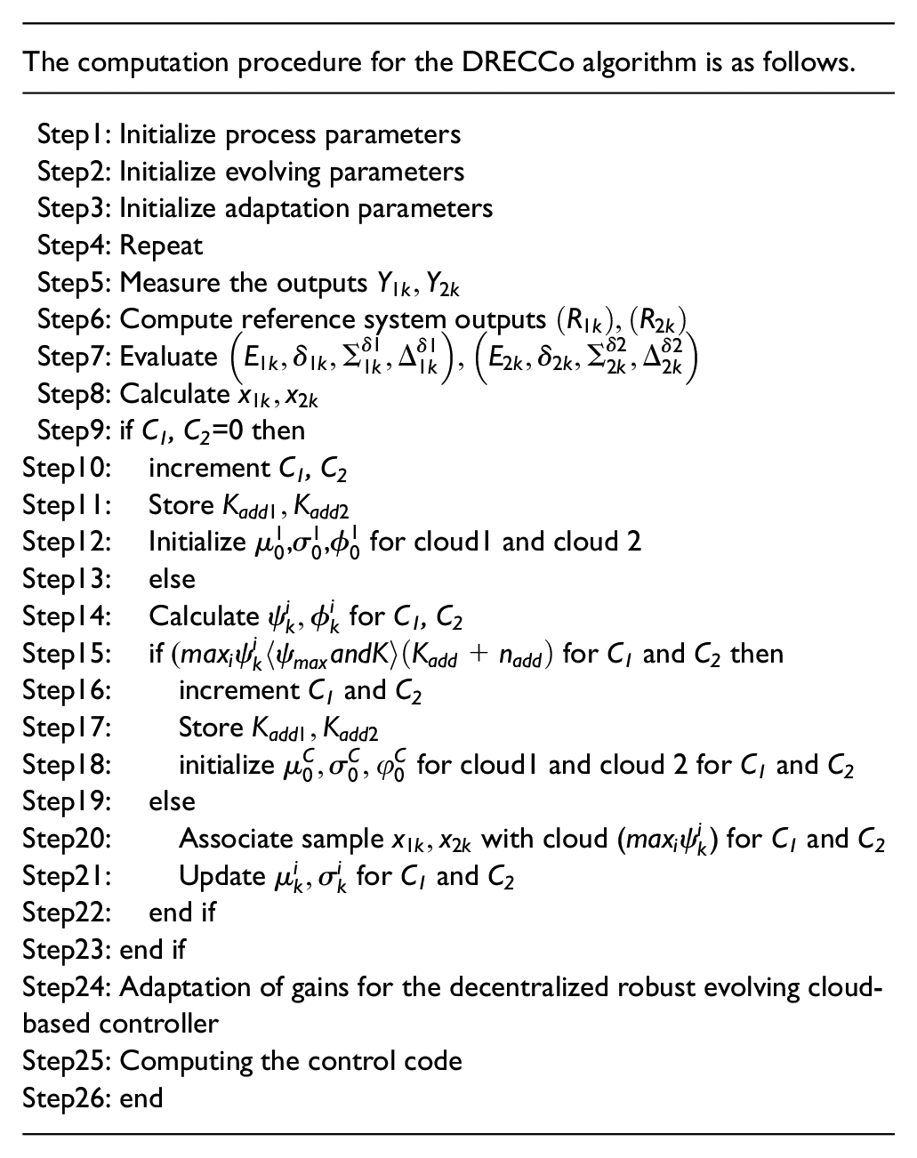
Computation procedure

Mathematical modeling

The modeling of the ITTP and QTP is illustrated in this section.

ITTP

The ITTP is a benchmark process for TITO systems comprised of two interlinked tanks and two pumps. In this type, two inputs are given to the two tanks separately and both the outputs are coupled together for interaction with each other. Figure 3 presents the schematic design of the ITTP. Tanks T₁ and T₂ were identical cylindrical tanks. These two tanks were interlinked using a manually operated valve. P₁ and P₂ are variable-frequency drive pumps feeding T₁ and T₂, respectively. The T₁ and T₂ tank levels are referred to as h₁ and h₂, respectively. The tank levels are maintained at a certain value by varying the input of the variable-frequency drives that control pumps P₁ and P₂, respectively.

For ITTP, the mass balance equation at an unsteady state is given by

A_{1} \frac{d h_{1}}{dt} = Q_{in 1} (t) - Q_{12} (t) - Q_{1} (t)

(32)

A_{2} \frac{d h_{2}}{dt} = Q_{in 2} (t) + Q_{12} (t) - Q_{2} (t)

(33)

The nonlinear equations are derived as

\begin{matrix} A_{1} \frac{d h_{1}}{dt} = k u_{1} (t) - k_{1} \sqrt{2 g h_{1} (t)} - sgn (h_{1} - h_{2}) k_{12} \\ \sqrt{2 g | h_{1} (t) - h_{2} (t) |} \end{matrix}

(34)

\begin{matrix} A_{2} \frac{d h_{2}}{dt} = k u_{2} (t) - k_{2} \sqrt{2 g h_{2} (t)} + sgn (h_{1} - h_{2}) k_{12} \\ \sqrt{2 g | h_{1} (t) - h_{2} (t) |} \end{matrix}

(35)

where h₁= height of Tank1 (cm), h₂ = height of Tank2 (cm), A₁= cross-sectional area (Tank1, cm²), A₂= cross-sectional area (Tank2, cm²), a₁= cross-sectional area (Tank1’s outlet, cm²), a₂= cross-sectional area (Tank2’s outlet, cm²),a₁₂ = cross-sectional area (interacting pipe (Tanks 1 and 2, cm²), Q_in1, Q_in2= tanks’ rate of inflow (cm³/s), g= specific gravity(cm³/s), k₁,k₂ = valve ratio of the outlet of Tanks 1 and 2, k₁₂ = interacting valve ratio= pump constant for Pumps1 and 2(cm³/v-s), u₁, u₂ = input voltage for Pumps 1 and 2 (volts).

QTP

The QTP is a benchmark process that comprises four interlinked tanks and two pumps. A schematic of the process is shown in Figure 4. The process inputs are $u_{1}, u_{2}$ and the outputs are . The aim was to maintain the heights of the two bottom tanks. There are two valves on either side that divide the inflow from the pumps into one bottom tank and one tank at the top (i.e., in the diagonal position). Each tank was fitted with a bottom-discharge valve. A valve was placed at the bottom of each tank. Tank 4 (T₄) is discharged to Tank1 (T₁), whereas Tank 3 (T₃) is discharged to Tank 2 (T₂). Such interaction provides a powerful connection between the tanks that form the system for multi-variable control. Hence, controlling and maintaining the levels of tanks in this process is a very challenging task. The stance of the two valves defines whether the system is in the minimum phase (MP) or non-minimum phase (NMP). The valve ratio of the first tank is $γ_{1}$ , and the valve ratio of the diagonal top tank (i.e., the fourth tank) is $(1 - γ_{1})$ . Similarly, the valve ratios for 2^nd and 4^th tanks are $γ_{2}$ and $(1 - γ_{2})$ , respectively.

From the basic first principles

\begin{matrix} \frac{d h_{1}}{dt} = \frac{1}{A_{1}} (γ_{1} b_{1} u_{1} + a_{3} \sqrt{2 g h_{3}} - a_{1} \sqrt{2 g h_{1}}) \\ \frac{d h_{2}}{dt} = \frac{1}{A_{2}} (γ_{2} b_{2} u_{2} + a_{4} \sqrt{2 g h_{4}} - a_{2} \sqrt{2 g h_{2}}) \\ \frac{d h_{3}}{dt} = \frac{1}{A_{3}} ((1 - γ_{2}) b_{2} u_{2} - a_{3} \sqrt{2 g h_{3}}) \\ \frac{d h_{4}}{dt} = \frac{1}{A_{4}} ((1 - γ_{1}) b_{1} u_{1} - a_{4} \sqrt{2 g h_{4}}) \end{matrix}

(36)

where $γ_{i}$ = flow splits (0 to 1), $g$ = gravitational force (981 cm/s²), $τ_{i}$ = time constants for Tanks 1 to 4, $τ_{i} = \frac{A_{i}}{a_{i}} \sqrt{\frac{2 h_{i}}{g}}$ , $b_{i}$ = pump constants, A₁ to A₄ = cross-sectional area of T₁ to T₄ = 8.96 cm², and a₁ to a₄ = outlet cross-sectional area of T₁ to T₄= 0.05 cm².

The transfer matrix is as follows

G (s) = [\begin{matrix} \frac{q_{1} γ_{1}}{(1 + s τ_{1})} & \frac{q_{1} (1 - γ_{2})}{(1 + s τ_{1}) (1 + s τ_{3})} \\ \frac{q_{2} (1 - γ_{1})}{(1 + s τ_{2}) (1 + s τ_{4})} & \frac{q_{2} γ_{2}}{(1 + s τ_{2})} \end{matrix}]

where

q_{1} = \frac{τ_{1} p_{c 1} b_{1}}{A_{1}}, q_{2} = \frac{τ_{2} p_{c 2} b_{2}}{A_{2}}

p_{ci} = \sqrt{\frac{2 h_{i}}{g}} = 0.507, 5.13

(38)

Results and discussions

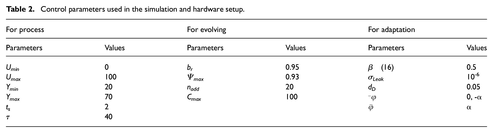
In this segment, the proposed DRECCo was implemented for two benchmark processes, and a reference signal with a flight of stairs was chosen to cover the maximum range of the process. The parameter values used for both the simulation and the hardware setup are presented in Table 2.

Table 2.

Control parameters used in the simulation and hardware setup.

For process		For evolving		For adaptation
Parameters	Values	Parameters	Values	Parameters	Values
U_min	0	b_r	0.95	β (16)	0.5
U_max	100	Ψ_max	0.93	σ_Leak	10^-6
Y_min	20	n_add	20	d_D	0.05
Y_max	70	C_max	100	${}^{-}φ$	0, -α
t_s	2			$\bar{φ}$	α
τ	40

The computation procedure for the DRECCo algorithm is as follows.
Step1: Initialize process parameters Step2: Initialize evolving parameters Step3: Initialize adaptation parameters Step4: Repeat Step5: Measure the outputs $Y_{1 k}, Y_{2 k}$ Step6: Compute reference system outputs $(R_{1 k}), (R_{2 k})$ Step7: Evaluate $(E_{1 k}, δ_{1 k}, Σ_{1 k}^{δ 1}, Δ_{1 k}^{δ 1}), (E_{2 k}, δ_{2 k}, Σ_{2 k}^{δ 2}, Δ_{2 k}^{δ 2})$ Step8: Calculate $x_{1 k}, x_{2 k}$ Step9: if C₁, C₂=0 thenStep10: increment C₁, C₂Step11: Store $K_{add 1}, K_{add 2}$ Step12: Initialize $μ_{0}^{1}$ , $σ_{0}^{1}$ , $ϕ_{0}^{1}$ for cloud1 and cloud 2Step13: elseStep14: Calculate $ψ_{k}^{i}, ϕ_{k}^{i}$ for C₁, C₂Step15: if $(ma x_{i} ψ_{k}^{i} 〈 ψ_{\max} and K 〉 (K_{add} + n_{add})$ for C₁ and C₂ thenStep16: increment C₁ and C₂Step17: Store $K_{add 1}, K_{add 2}$ Step18: initialize $μ_{0}^{C}, σ_{0}^{C}, φ_{0}^{C}$ for cloud1 and cloud 2 for C₁ and C₂Step19: elseStep20: Associate sample $x_{1 k}, x_{2 k}$ with cloud ( $ma x_{i} ψ_{k}^{i}$ ) for C₁ and C₂Step21: Update $μ_{k}^{i}, σ_{k}^{i}$ for C₁ and C₂Step22: end ifStep23: end ifStep24: Adaptation of gains for the decentralized robust evolving cloud-based controllerStep25: Computing the control codeStep26: end

The computation procedure for the DRECCo algorithm is as follows.

Step1: Initialize process parameters Step2: Initialize evolving parameters Step3: Initialize adaptation parameters Step4: Repeat Step5: Measure the outputs

Y_{1 k}, Y_{2 k}

Step6: Compute reference system outputs

(R_{1 k}), (R_{2 k})

Step7: Evaluate

(E_{1 k}, δ_{1 k}, Σ_{1 k}^{δ 1}, Δ_{1 k}^{δ 1}), (E_{2 k}, δ_{2 k}, Σ_{2 k}^{δ 2}, Δ_{2 k}^{δ 2})

Step8: Calculate

x_{1 k}, x_{2 k}

Step9: if C₁, C₂=0 thenStep10: increment C₁, C₂Step11: Store

K_{add 1}, K_{add 2}

Step12: Initialize

μ_{0}^{1}

σ_{0}^{1}

ϕ_{0}^{1}

for cloud1 and cloud 2Step13: elseStep14: Calculate

ψ_{k}^{i}, ϕ_{k}^{i}

for C₁, C₂Step15: if

(ma x_{i} ψ_{k}^{i} 〈 ψ_{\max} and K 〉 (K_{add} + n_{add})

for C₁ and C₂ thenStep16: increment C₁ and C₂Step17: Store

K_{add 1}, K_{add 2}

Step18: initialize

μ_{0}^{C}, σ_{0}^{C}, φ_{0}^{C}

for cloud1 and cloud 2 for C₁ and C₂Step19: elseStep20: Associate sample

x_{1 k}, x_{2 k}

with cloud (

ma x_{i} ψ_{k}^{i}

) for C₁ and C₂Step21: Update

μ_{k}^{i}, σ_{k}^{i}

for C₁ and C₂Step22: end ifStep23: end ifStep24: Adaptation of gains for the decentralized robust evolving cloud-based controllerStep25: Computing the control codeStep26: end

Hardware setup

The hardware setup used for the two benchmark processes is illustrated in Figure 6. It is a multitank setup that can be made to operate in several configurations by adjusting the ball valves. The bottom tanks T₁ and T₂ are used for the ITTP. For the QTP, four cylindrical tanks (T₁, T₂, T₃, and T₄) were configured as shown in Figure 5. Pressure transmitters (LT₁ and LT₂) were used to measure the height of the tanks. They are calibrated such that a maximum height of 38 cm gives a value of 100% (i.e., 100%=38cm). The input flow rates can be adjusted by setting the frequency of the variable-frequency drives (VFD) running the pumps. The hardware setup was interfaced with a computer running Laboratory Virtual Instrument Engineering Workbench (LabVIEW). All the preliminary parameters that were provided during the simulation were provided as initial parameters while performing the experiments.

The open-loop response for the ITTP is shown in Figure 5. The heights (h₁, h₂) of the tanks (T₁ and T₂) were initially maintained at 50% and 40% of their rated height, respectively, by running the pumps (P₁, P₂) at 50% and 40% of their rated speed using variable-frequency drive 1 (VFD1) and variable-frequency drive2 (VFD2), respectively. Then, the speed of P₁ is changed from 50% to 60% of its rated speed by keeping the P₂ speed constant, and the heights of the tanks are logged. The same procedure is repeated by changing the speed of P₂ from 40% to 50% of its rated speed by keeping the P₁ speed constant.

Loop interaction analysis (ITTP)

The interaction in the process brings the system to nonlinear behavior; hence, it is important to pair the exact input to control the exact output. The relative-gain array (RGA) is a classical method for selecting the optimal input-output pairing for multi-variable process control systems, which is denoted as ( $\land_{RGA}$ ). This is determined as the proportion between the gains of input ( $u_{i}$ ) and output ( $y_{i}$ ) when all the variant connections are opened on one hand and the gains of the same input ( $u_{j}$ ) and output ( $y_{j}$ ) when all the variant connections are blocked on the other hand. For I/O pairing, the controller required a model.

The transfer function is taken from the open-loop response of the ITTP

G (s) = [\begin{matrix} \frac{0.5781}{54.1 s + 1} & \frac{0.0693}{(54.1 s + 1) (51.29 s + 1)} \\ \frac{0.0629}{(50.91 s + 1) (51.86 s + 1)} & \frac{0.0707}{51.86 s + 1} \end{matrix}]

(39)

The steady-state gain matrix is given by putting s=0 in (34)

G (0) = [\begin{matrix} 0.5781 & 0.0693 \\ 0.0692 & 0.0707 \end{matrix}]

(40)

The output is represented as

\begin{matrix} y_{1} = g_{11} u_{1} + g_{11} u_{2} \\ y_{2} = g_{21} u_{1} + g_{22} u_{2} \end{matrix}

(41)

where g_ij=steady-state gains of the process transfer function G(s)

g = [\begin{matrix} g_{11} & g_{12} \\ g_{21} & g_{22} \end{matrix}]

(42)

\land_{RGA} = g * R

(43)

where * is the scur product

R = (g^{- 1})^{T}

(44)

\land_{RGA} = [\begin{matrix} λ_{11} & λ_{12} \\ λ_{21} & λ_{22} \end{matrix}]

(45)

\land_{RGA} = [\begin{matrix} 1.13 & - 0.13 \\ - 0.13 & 1.13 \end{matrix}]

(46)

The below is from the guidelines to be adopted for input-output pairs (Luyben, 1999; Kadhim et al., 2016; Seborg and Edgar, 2011):

Select the matching input-output pairs that are suited to the RGA elements closer to 1.

Avoid coupling with vast or pessimistic RGA elements.

Therefore, in the decentralized loop control, the control input $u_{1}$ is paired with $y_{1}$ and the control input $u_{2}$ is paired with $y_{2}$ . In the QTP, the transmission is zero of the system MP and NMP, which is based on the valve positions. The operating points for the QTP at the MP and the transfer function are determined as follows

γ_{1} = 0.7, γ_{2} = 0.6

b_{1} = 3.3, b_{2} = 3.35

h_{10} = 12.4, h_{20} = 12.7, h_{30} = 1.8, h_{40} = 1.4

u_{1} = u_{2} = 10

τ_{1} = 27.9, τ_{2} = 28.6, τ_{3} = 10.68, τ_{4} = 9.29

q_{1} = 7.25, q_{2} = 6.42

G (s) = [\begin{matrix} \frac{5.075}{(1 + 27.9 s)} & \frac{2.9}{(1 + 27.9 s) (1 + 10.6 s)} \\ \frac{1.93}{(1 + 28.6 s) (1 + 9.3 s)} & \frac{3.85}{(1 + 28.6 s)} \end{matrix}]

(47)

The operating points for the QTP at the NMP and transfer function are resolved as follows

\begin{matrix} γ_{1} = 0.4, γ_{2} = 0.3 \\ b_{1} = 3.14, b_{2} = 3.29 \\ h_{10} = 12.6, h_{20} = 13, h_{30} = 4.8, h_{40} = 4.9 \\ u_{1} = u_{2} = 10 \\ τ_{1} = 28.32, τ_{2} = 28.77, τ_{3} = 17.48, τ_{4} = 17.66 \\ q_{1} = 5.032, q_{2} = 5.419 \\ G (s) = [\begin{matrix} \frac{2.013}{(1 + 28.32 s)} & \frac{3.52}{(1 + 28.32 s) (1 + 17.48 s)} \\ \frac{3.25}{(1 + 28.77 s) (1 + 17.66 s)} & \frac{3.85}{(1 + 28.77 s)} \end{matrix}] \end{matrix}

The interaction of loops (QTP)

The RGA for the MP to maintain the height of the tanks is as follows

g = [\begin{matrix} 5.075 & 2.9 \\ 1.93 & 3.85 \end{matrix}]

(49)

\land_{RGA} = [\begin{matrix} 1.4 & - 0.4 \\ - 0.4 & 1.4 \end{matrix}]

(50)

From this analysis, the control input u₁ is paired with output y₁, and the control input u₂ is paired with output y₂.

The RGA for the NMP to maintain the height of the tanks is as follows

g = [\begin{matrix} 2.013 & 3.52 \\ 3.25 & 1.63 \end{matrix}]

(51)

\land_{RGA} = [\begin{matrix} - 0.4 & 1.4 \\ 1.4 & - 0.4 \end{matrix}]

(52)

Therefore, in the decentralized loop control, the control input u₁ is paired with y₂, and the control input u₂ is paired with y₁.

Simulation results

The simulation starts with zero fuzzy rules. The membership functions were automatically learned and adapted to throughout the simulation process. The dead zone (d_D) was selected as 1% of the process range. The minimum and maximum bound are chosen as 0 and ∞ for the PID controller gains; at the same time, compensation gain is -∞ for minimum bound and the σ_Leak is given as 10^-6. The algorithm was examined using integral performance indices.

Integral absolute error (IAE) is as follows

IAE = t_{s} \sum_{k} | E_{k} |

(53)

Integral squared error (ISE) is as follows

ISE = t_{s} \sum_{k} | E_{k}^{2} |

(54)

where $E_{k} = R_{k} - Y_{k}$ is the error and t_s =2s is the sampling time.

For ITTP

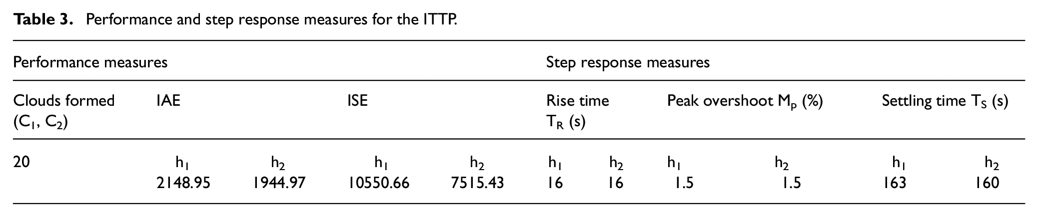
The closed-loop response along with the step change and output perturbation of the proposed controller is shown in Figure 7. The top plots in the figure show the desired set points, the response of the reference models, and the response of the process. The middle plots similarly show the control actions, and the tracking errors are depicted in the lower plots. The step changes in set points are applied at regular intervals (500 s) until the 2500 s and irregular intervals for the remaining period. Positive step disturbances of magnitude 2 cm were added to the output at 130 s and 1800 s, respectively. Similarly, negative step disturbances of magnitude 2 cm were added to the output at 3100 s and 3600 s, respectively. It can be observed from the figures that even if the controller is started with zero fuzzy rules and with bare minimum knowledge of interaction, it is capable of building the fuzzy rules and tracking the reference model output and eliminating the effect of disturbances in the outputs. The formation of clouds is shown in Figure 8. Table 3 shows the performance and step response measures of the proposed controller for the second step (i.e., 500–1000 s).

Table 3.

Performance and step response measures for the ITTP.

Performance measures					Step response measures
Clouds formed(C₁, C₂)	IAE		ISE		Rise timeT_R (s)		Peak overshoot M_p (%)		Settling time T_S (s)
20	h₁	h₂	h₁	h₂	h₁	h₂	h₁	h₂	h₁	h₂
	2148.95	1944.97	10550.66	7515.43	16	16	1.5	1.5	163	160

Robustness of the proposed controller

The unique feature of the ITTP is that, based on the height of the liquid level in both tanks, the direction of the interflow between the tanks reverses, which results in a discrete jump of the process model from one mode to another. To test the robustness of the DRECCo against the discrete change in the dynamics of the process, a step change is initially provided such that h₁>h₂. Once the process is settled, another step change is applied, such that h₂>h₁. That is, in the beginning, the height of T₁ is 25 cm and that of T₂ is 15 cm until 750 s. After that, the reference height of tank T₁ was set as 15 cm and that of T₂ was set as 20 cm, and the results are shown in Figure 9. Because the controller starts with zero fuzzy rules, it takes some time for the controller to learn. During the first step, the response has more overshoot. Once the controller has learned some information, it is capable of tracking the reference model outputs, as can be observed from the second step. In addition, a step disturbance of +2 is applied to the first tank output between400 s and 600 s. Again, a step disturbance of -3 was applied between1100 s and 1300 s in the second tank output. The proposed controller maintained the level of both tanks.

For QTP

The closed-loop responses for MP and NMP are shown in Figures 10 and 11, respectively, in which the top plots show the desired set points, the output of the reference models, and the responses of the process. Likewise, the middle plots show the control actions and tracking errors in the lower plots. Step changes in set points are applied at regular intervals (500 s) until 2500 s and irregular intervals for the remaining period. Positive step disturbances of magnitude 3 cm were added to the output at 1300 s and 1800 s, respectively.

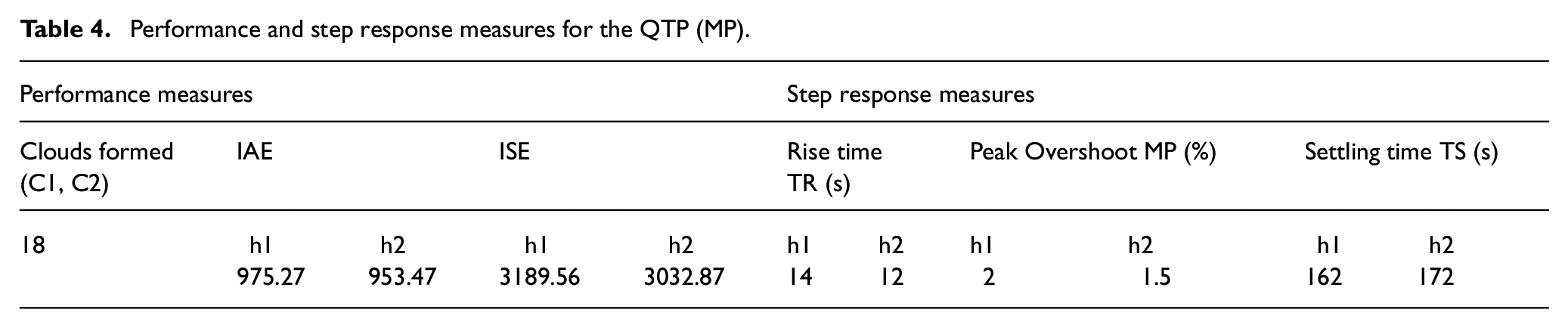
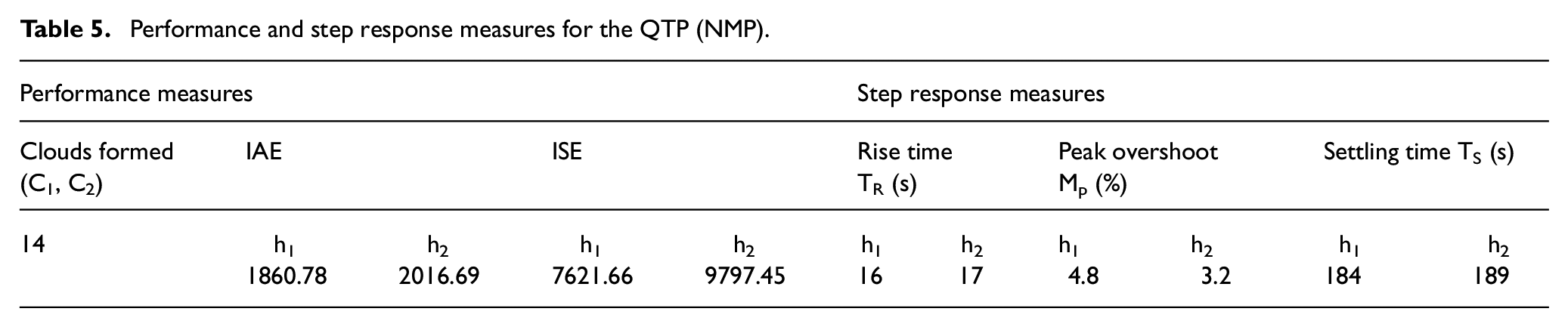
Similarly, negative step disturbances of magnitude 3 cm were added to the output at 3200 s and 3800 s, respectively. From the figures, it can be observed that even if the controller is started with zero fuzzy rules and with bare minimum knowledge of interaction, it is capable of building the fuzzy rules and tracking the reference model output in addition to eliminating the effect of disturbances in the outputs. For the second step, that is, 500 to 1000 s, the performance and step response measures for the MPand NMP are tabulated in Tables 4 and 5.

Table 4.

Performance and step response measures for the QTP (MP).

Performance measures					Step response measures
Clouds formed(C1, C2)	IAE		ISE		Rise timeTR (s)		Peak Overshoot MP (%)		Settling time TS (s)
18	h1	h2	h1	h2	h1	h2	h1	h2	h1	h2
	975.27	953.47	3189.56	3032.87	14	12	2	1.5	162	172

Table 5.

Performance and step response measures for the QTP (NMP).

Performance measures					Step response measures
Clouds formed(C₁, C₂)	IAE		ISE		Rise timeT_R (s)		Peak overshootM_p (%)		Settling time T_S (s)
14	h₁	h₂	h₁	h₂	h₁	h₂	h₁	h₂	h₁	h₂
	1860.78	2016.69	7621.66	9797.45	16	17	4.8	3.2	184	189

Hardware results

For ITTP

Initially, the process was started under an open loop. When the process is in a steady state, a DRECCo is turned ON. The response of the process after the DRECCo is turned ON as shown in Figure 12. It shows the desired set points, the response of the reference models, and the response of the process. Step changes in set points are applied at irregular intervals, and an external disturbance of 350 ml and 400 ml of water was added to T₁ and T₂ at 750 s and 1050 s, respectively. From the graph, it can be observed that the reference model is tracked, and disturbances are eliminated.

For QTP

Figures 13 and 14 show the closed-loop responses of the QTP for MP and NMP, respectively, which show the desired set points, the output of the reference models, and the responses of the process. Step changes in the set points were applied at irregular intervals. At external disturbance of 400 ml, 350 ml of water is added in Tank 1 and Tank 2 at 900 s and 500 s, respectively, for the MP. For the NMP, an external disturbance of 400 ml of water is added in both tanks at 700 s and 980 s, respectively. From the graph, it can be observed that the output tracks the reference model and eliminates disturbances.

Conclusion

In this study, a DRECCo was proposed. The key benefit of the proposed controller is that it requires minimum initial parameters, such as loop pairing information based on an approximate model and can start with zero antecedent parameters and fuzzy rules. The DRECCo was implemented on two benchmark nonlinear processes (ITTP and QTP) in the simulation as well as in the hardware setup. Reference model tracking and disturbance rejection responses are presented. It can be observed that a DRECCo can track the reference model output for the entire operating range once it learns some information about the process. The robustness of DRECCo against disturbances and variations in process dynamics was also discussed. However, a DRECCo has limitations in its ability to overcome strong interactions, as in any other decentralized controller. Future research may focus on developing centralized RECCo that can operate against strong interactions, even with zero process knowledge.

Footnotes

Acknowledgements

The authors express their gratitude to Thiagarajar College of Engineering, India, for their extensive support. The authors take this opportunity to express their sincere gratitude to Dr S. Baskar and Mr M. Varatharajan for their valuable guidance.

Declaration of conflicting interests

The author(s) declared no potential conflicts of interest with respect to the research, authorship, and/or publication of this article.

Funding

The author(s) disclosed receipt of the following financial support for the research, authorship, and/or publication of this article: This work was supported by The Institute of Engineers (INDIA) IEI R&D Grant-in-Aid Scheme, (Ref: R.6/2/DR/2019-20/DR2020015, dated 7 February 2020).

ORCID iD

J Vijay Anand

References

Andonovski

Costa

BSJ

(2017) Robust evolving control of a two-tanks pilot plant. In: IEEE Conference on Evolving and Adaptive Intelligent Systems 2017, Ljubljana, Slovenia, 31 May–2 June 2017, pp. 1–7. IEEE.

Andonovski

, et al. (2015a) Analysis of adaptation law of the robust evolving cloud-based controller. In: 2015 IEEE International Conference on Evolving and Adaptive Intelligent Systems, EAIS 2015, Douai, France, 1–3 December 2015, pp. 1–7. IEEE.

Andonovski

, et al. (2015b) Robust evolving cloud-based controller in normalized data space for heat-exchanger plant. In: IEEE International Conference on Fuzzy Systems (FUZZ-IEEE), Istanbul, Turkey, 2–5 August 2015, pp. 1–7. IEEE.

Andonovski

, et al. (2016a) A practical implementation of robust evolving cloud-based controller with normalized data space for heat-exchanger plant. Applied Soft Computing 48: 29–38.

Andonovski

, et al. (2016b) Robust evolving cloud-based control for the distributed solar collector field. In: 2016 IEEE International Conference on Fuzzy Systems (FUZZ-IEEE), Vancouver, BC, Canada, 24–29 July 2016, pp. 1570–1577. IEEE.

Andonovski

, et al. (2016c) On-line evolving cloud-based model identification for production control. IFAC-PapersOnLine 49(5): 79–84.

Andonovski

, et al. (2017) Robust evolving cloud-based controller (RECCo). In: IEEE Conference on Evolving and Adaptive Intelligent Systems (EAIS), Ljubljana, Slovenia, 31 May–2 June 2017, pp. 1–6.

Andonovski

, et al. (2018) Robust evolving controller for simulated surge tank and for real two-tank plant. At-Automatisierungstechnik 66(9): 725–734.

Angelov

Yager

(2011) Simplified fuzzy rule-based systems using non-parametric antecedents and relative data density. In: IEEE SSCI 2011: Symposium Series on Computational Intelligence – EAIS 2011: 2011 IEEE Workshop on Evolving and Adaptive Intelligent Systems, Paris, France, 11–15 April 2011, pp. 62–69.

10.

Angelov

Yager

(2012) A new type of simplified fuzzy rule-based system. International Journal of General Systems 41(2): 163–185.

11.

Angelov

Škrjanc

Blažič

(2013) Robust evolving cloud-based controller for a hydraulic plant. In: IEEE Conference on Evolving and Adaptive Intelligent Systems (EAIS), Singapore, 16–19 April 2013, pp. 1–8.

12.

Astrom

Johansson

Wang

(2002) Design of decoupled PI controllers for two-by-two systems. IEE Proceedings: Control Theory and Applications 149(1): 74–81.

13.

Basci

Derdiyok

(2016) Implementation of an adaptive fuzzy compensator for coupled tank liquid level control system. Measurement: Journal of the International Measurement Confederation 91: 12–18.

14.

Bhattacharya

Chatterjee

Munshi

(2003) An improved PID-type fuzzy controller employing individual fuzzy P, fuzzy I and fuzzy D controllers. Transactions of the Institute of Measurement & Control 25(4): 352–372.

15.

Cara

Pomares

Rojas

(2011) A new methodology for the online adaptation of fuzzy self-structuring controllers. IEEE Transactions on Fuzzy Systems 19(3): 449–464.

16.

Cara

, et al. (2010) Online self-evolving fuzzy controller with global learning capabilities’, Evolving Systems 1(4): 225–239.

17.

Costa

, et al. (2013) A practical implementation of self-evolving cloud-based control of a pilot plant. In: 2013 IEEE International Conference on Cybernetics, CYBCONF 2013, Yogyakarta, Indonesia, 3–4 December 2013, pp. 7–12.

18.

Hajare

Patre

(2015) Decentralized PID controller for TITO systems using characteristic ratio assignment with an experimental application. ISA Transactions 59: 385–397.

19.

Ioannou

Kokotovic

(1984) Instability analysis and improvement of robustness of adaptive control. Automatica 20(5): 583–594.

20.

Johansson

(2000) The quadruple-tank process: A multivariable laboratory process with an adjustable zero. IEEE Transactions on Control Systems Technology 8(3): 456–465.

21.

Johansson

, et al. (1999) Teaching multivariable control using the quadruple-tank process. In: Proceedings of the IEEE Conference on Decision and Control, Arizona, USA, 7–10 December 1999, Vol. 1, pp. 807–812.

22.

Johansson

Nunes

JLR

(1998) A multivariable laboratory process with an adjustable zero. Proceedings of the American Control Conference4(3): 2045–2049.

23.

Kadhim

AMH

Birk

Arranz

(2016) Dynamic relative gain array estimation using local polynomial approximation approach. Modeling, Identification and Control 37(4): 247–259.

24.

Kayacan

Kaynak

(2009) An adaptive grey PID-type fuzzy controller design for a non-linear liquid level system. Transactions of the Institute of Measurement & Control 31(1): 33–49.

25.

Kreisselmeier

Narendra

(1982) Stable model reference adaptive control in the presence of bounded disturbances. IEEE Transactions on Automatic Control 27(6): 1169–1175.

26.

Luyben

(1999) Process Modeling, Simulation and Control for Chemical Engineers. 2nd edn. Singapore: McGraw-Hill International Editions.

27.

Mahapatro

Subudhi

Ghosh

(2019) Design and experimental realization of a robust decentralized PI controller for a coupled tank system. ISA Transactions 89: 158–168.

28.

Musmade

Patre

(2013) Feedforward-plus-sliding mode controller design with experimental application of coupled tank system. Transactions of the Institute of Measurement and Control 35(8): 1058–1067.

29.

Peterson

Narendra

(1982) Bounded error adaptive control. IEEE Transactions on Automatic Control 27(6): 1161–68.

30.

Rohrs

Valavani

Athans

Stein

(1985) Robustness of continuous-time adaptive control algorithms in the presence of unmodeled dynamics. IEEE Transactions on Automatic Control 30(9): 881–889.

31.

Ross

(2010) Fuzzy Logic with Engineering Applications. 3rd edn. United Kingdom: John Wiley & Sons, Ltd.

32.

Seborg

Edgar

(2011) Process Dynamics and Control Third Edition Dale. John Wiley & Sons, Inc, USA.

33.

Skrjanc

Blazic

Angelov

(2014) Robust evolving cloud-based PID control adjusted by gradient learning method. In: 2014 IEEE Conference on Evolving and Adaptive Intelligent Systems, IEEE EAIS 2014 – Conference Proceedings, Linz, Austria, 2–4 June 2014, pp. 1–8.

34.

Zhang

Chi

(2020) Model-free adaptive PID control for nonlinear discrete-time systems. Transactions of the Institute of Measurement and Control 42(10): 1797–1807.

35.

Zheng

Tang

Song

(2016) Graphical tuning method for non-linear fractional-order PID-type controllers free of analytical model. Transactions of the Institute of Measurement and Control 38(12): 1442–1459.

36.

Zhou

, et al. (2015) Fast gradient-based distributed optimisation approach for model predictive control and application in four-tank benchmark. IET Control Theory and Applications 9(10): 1579–1586.